Deep Convolutional Neural Network for Mapping Smallholder Agriculture Using High Spatial Resolution Satellite Image


Abstract
1. Introduction
2. Data
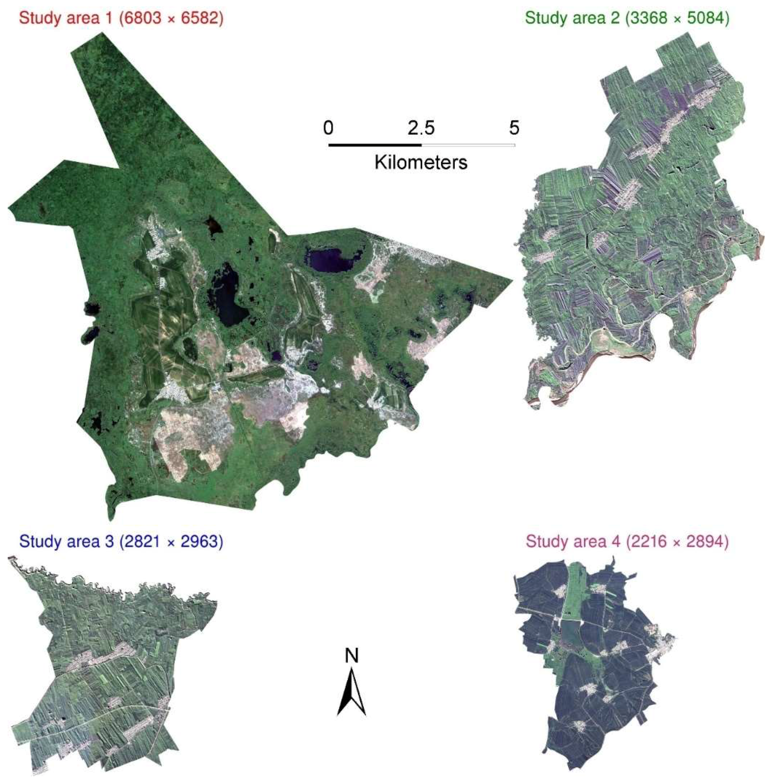
2.1. Study Areas
2.2. GaoFen-1 Data
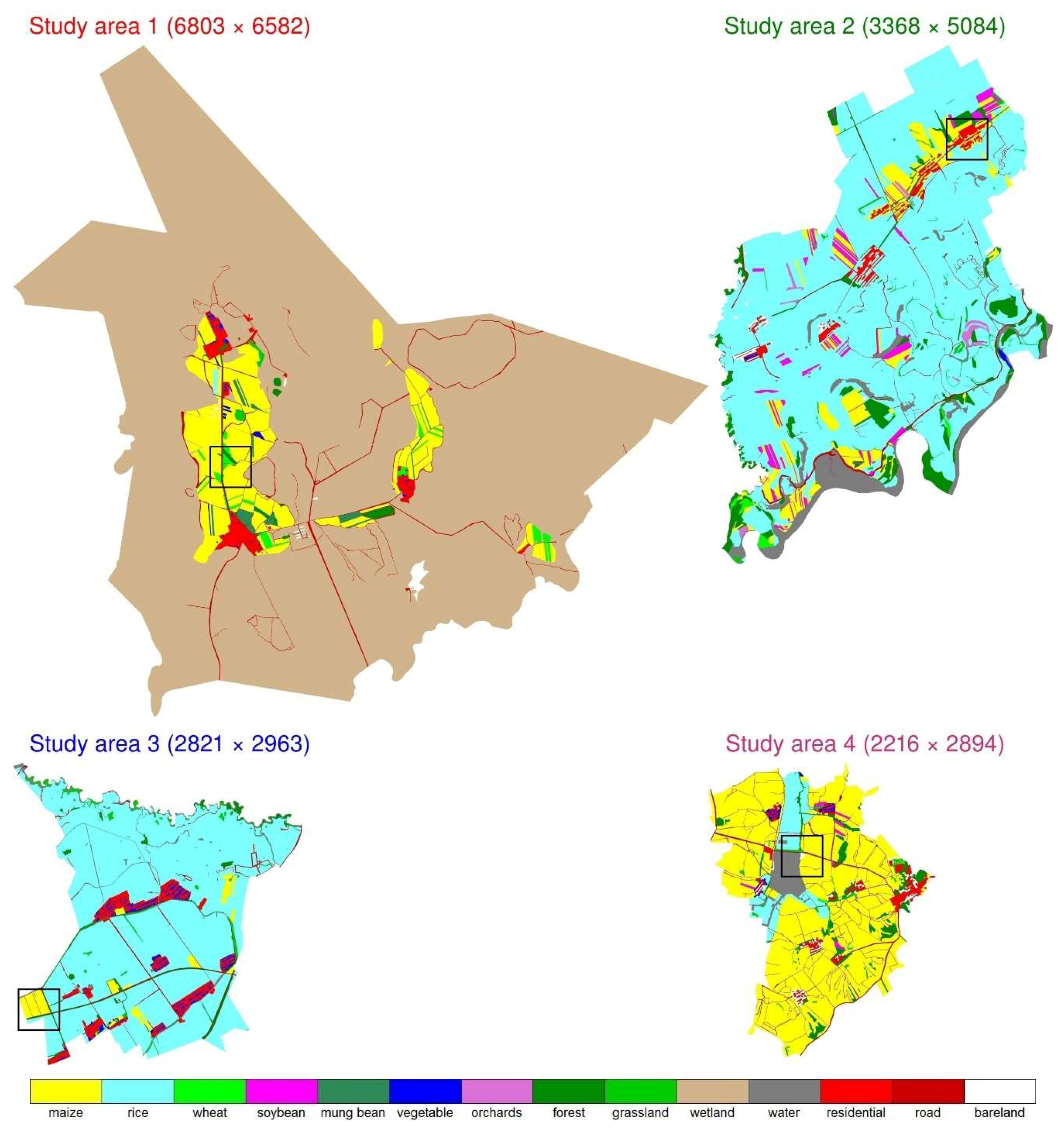
2.3. Reference Land Cover Maps for Training and Testing
3. Methods
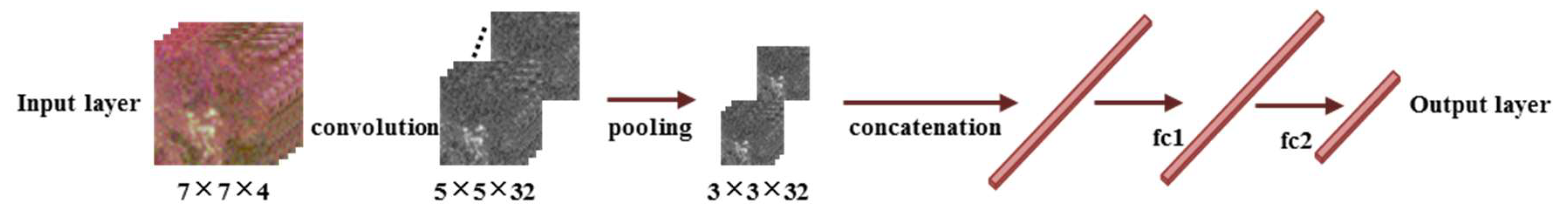
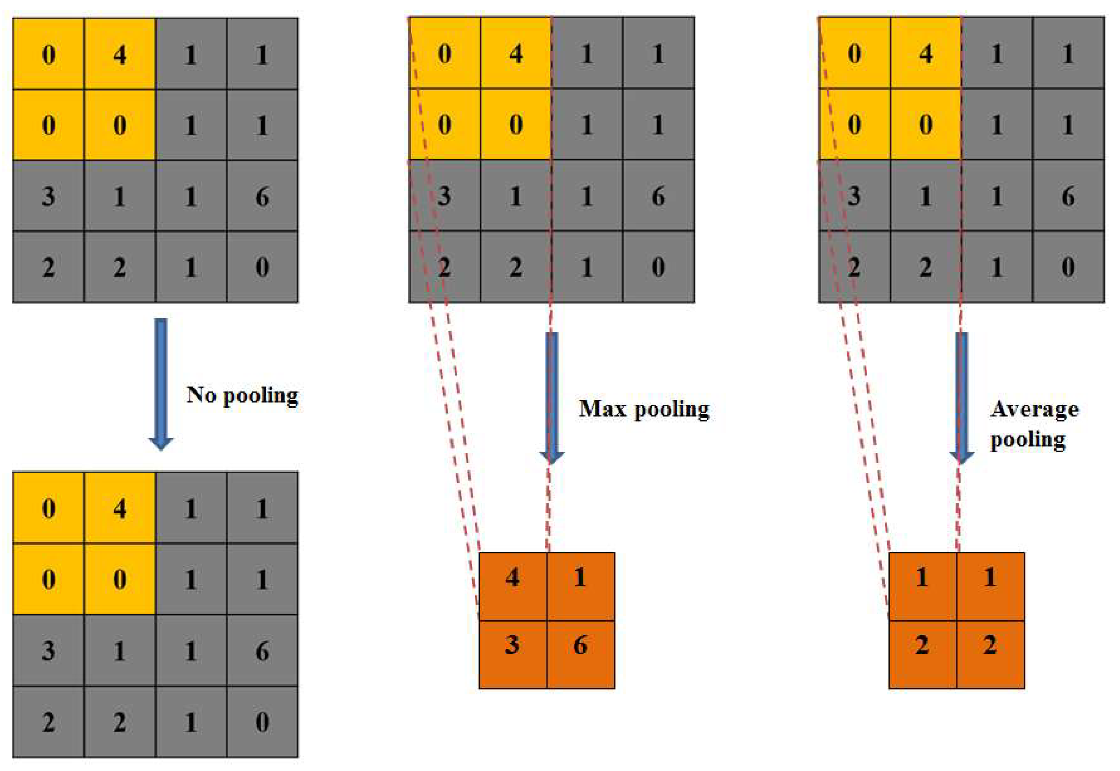
3.1. CNN Overview
3.2. CNN Structure Parameter Tuning
3.3. CNN Training Parameterization
3.4. Classification Result Evaluation
4. Results
4.1. CNN Structure Parameter Tuning
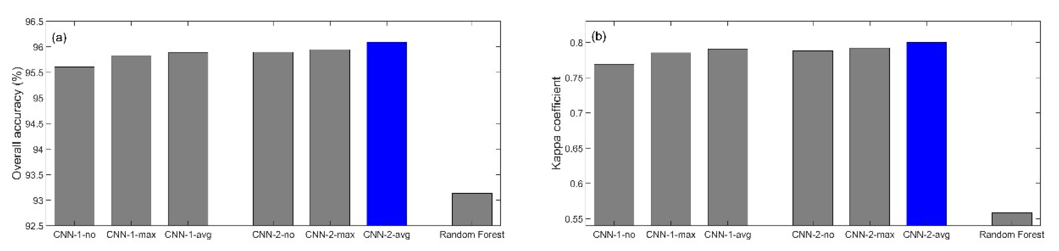
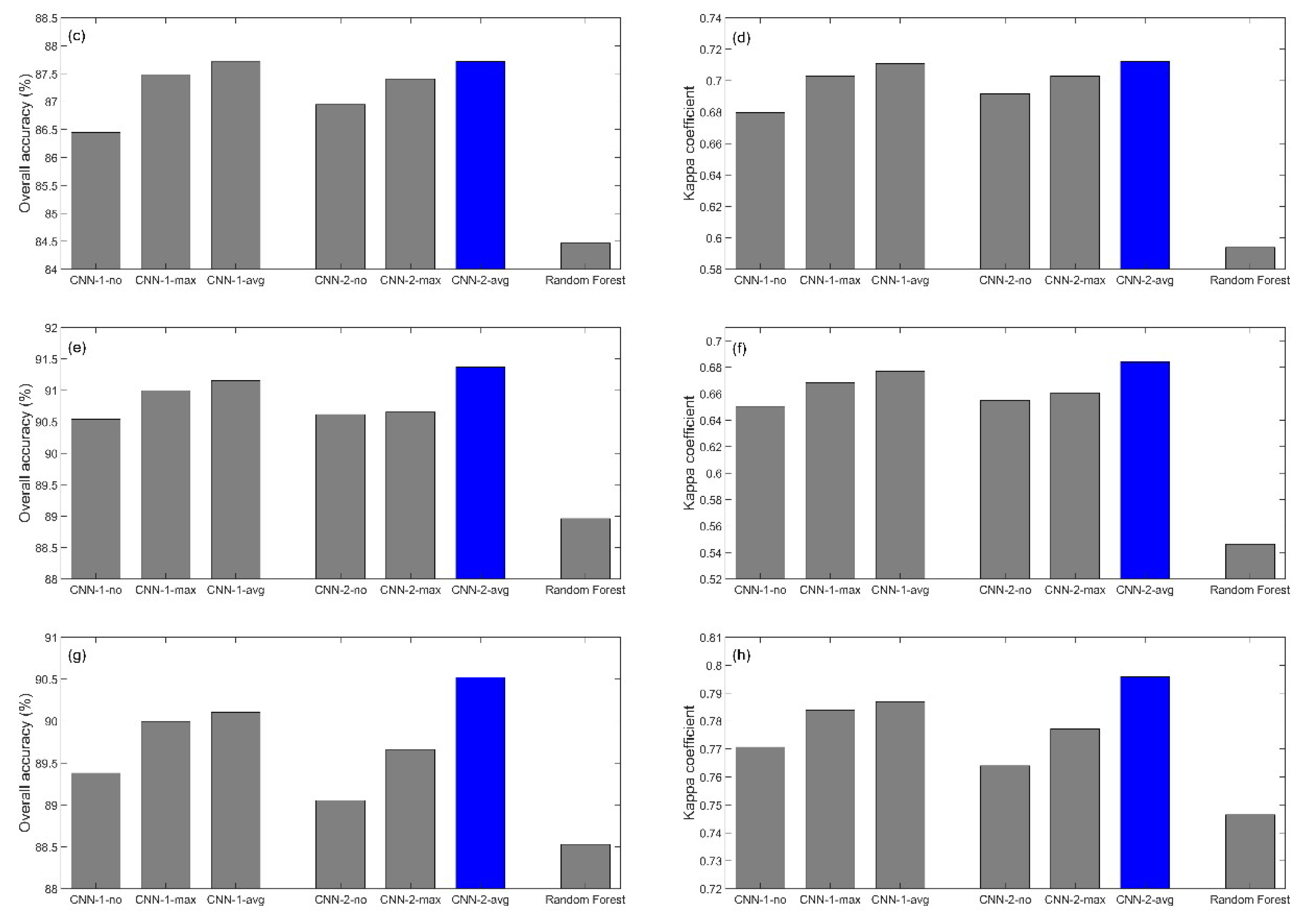
4.2. CNN and Random Forest Classification Accuracy Comparison
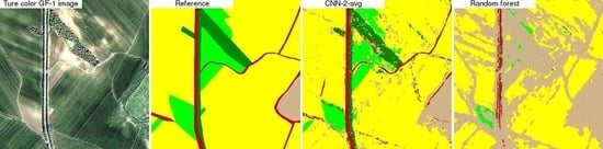
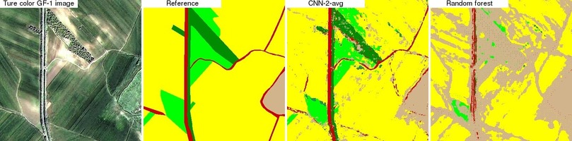
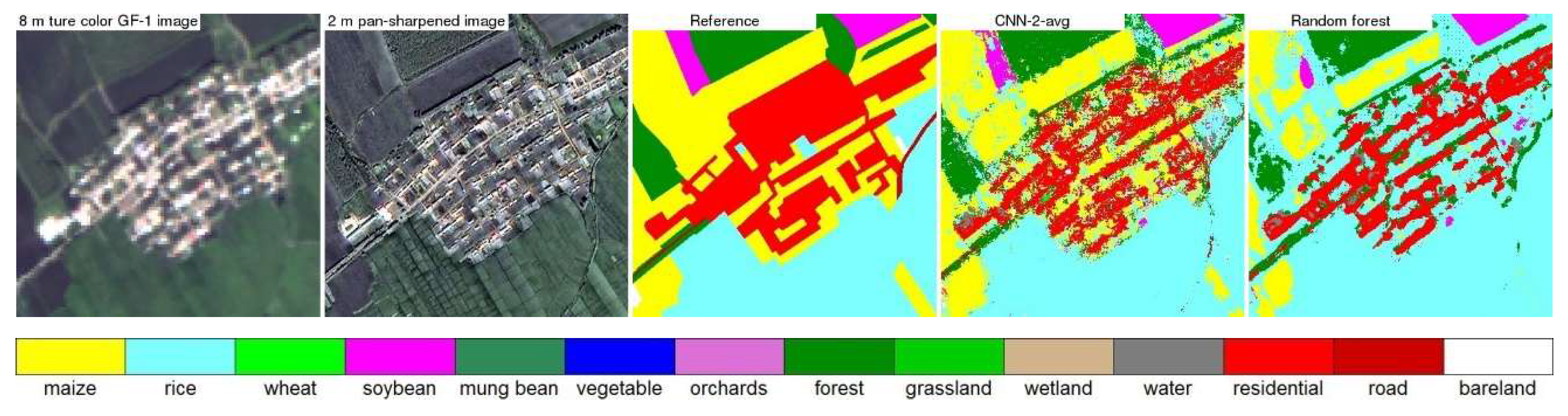
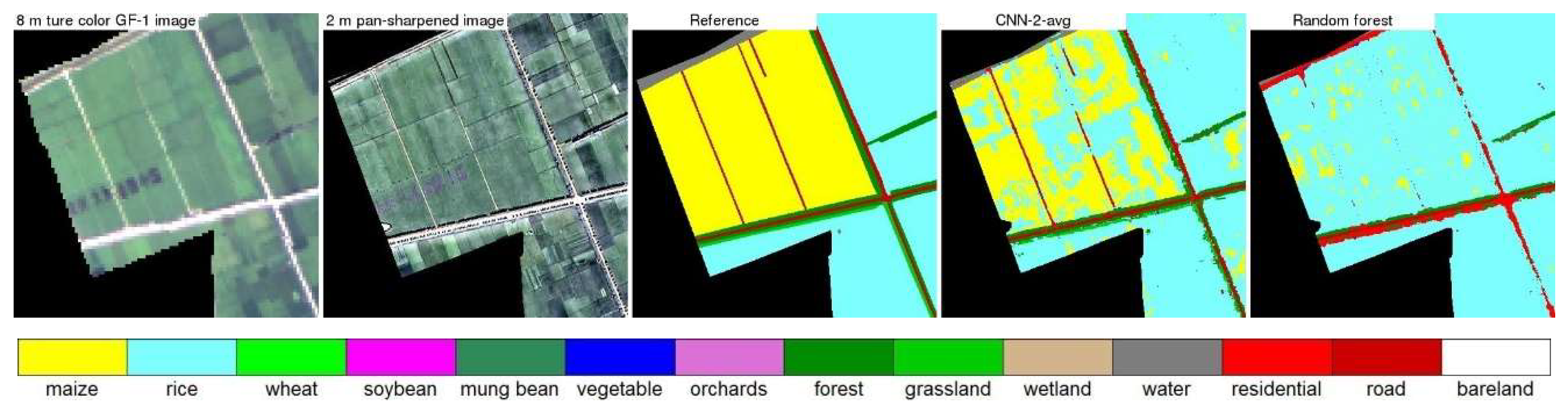
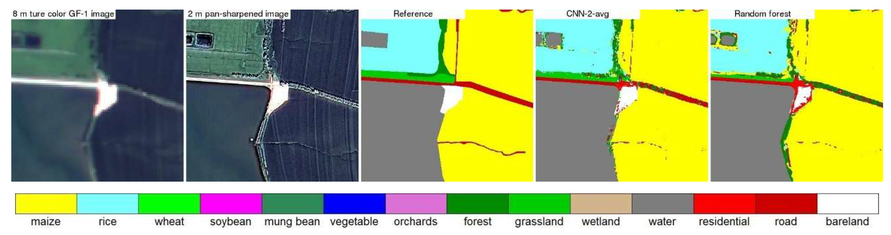
4.3. CNN and Random Forest Land Cover Map Comparison
4.4. CNN and Random Forest Accuracy Comparison for Balanced Training Data
5. Discussion
6. Conclusions
Author Contributions
Funding
Conflicts of Interest
References
- Hansen, M.C.; Loveland, T.R. A review of large area monitoring of land cover change using Landsat data. Remote Sens. Environ. 2012, 122, 66–74. [Google Scholar] [CrossRef]
- Gómez, C.; White, J.C.; Wulder, M.A. Optical remotely sensed time series data for land cover classification: A review. ISPRS J. Photogramm. Remote Sens. 2016, 116, 55–72. [Google Scholar] [CrossRef]
- Phiri, D.; Morgenroth, J. Developments in Landsat land cover classification methods: A review. Remote Sens. 2017, 9, 967. [Google Scholar] [CrossRef]
- Wulder, M.A.; Coops, N.C.; Roy, D.P.; White, J.C.; Hermosilla, T. Land cover 2.0. Int. J. Remote Sens. 2018, 39, 4254–4284. [Google Scholar] [CrossRef]
- Bauer, M.E.; Cipra, J.E.; Anuta, P.E.; Etheridge, J.B. Identification and area estimation of agricultural crops by computer classification of Landsat MSS data. Remote Sens. Environ. 1979, 8, 77–92. [Google Scholar] [CrossRef]
- Hansen, M.C.; Potapov, P.V.; Moore, R.; Hancher, M.; Turubanova, S.A.; Tyukavina, A.; Kommareddy, A.; Thau, D.; Stehman, S.V.; Goetz, S.J.; et al. High-resolution global maps of 21st-century forest cover change. Science 2013, 342, 850–853. [Google Scholar] [CrossRef] [PubMed]
- Hermosilla, T.; Wulder, M.A.; White, J.C.; Coops, N.C.; Hobart, G.W. Disturbance-Informed Annual Land Cover Classification Maps of Canada’s Forested Ecosystems for a 29-Year Landsat Time Series. Can. J. Remote Sens. 2018, 44, 67–87. [Google Scholar] [CrossRef]
- Gong, P.; Wang, J.; Yu, L.; Zhao, Y.; Zhao, Y.; Liang, L.; Niu, Z.; Huang, X.; Fu, H.; Liu, S.; et al. Finer resolution observation and monitoring of global land cover: First mapping results with Landsat TM and ETM+ data. Int. J. Remote Sens. 2013, 34, 2607–2654. [Google Scholar] [CrossRef]
- Chen, J.; Chen, J.; Liao, A.; Cao, X.; Chen, L.; Chen, X.; He, C.; Han, G.; Peng, S.; Lu, M. Global land cover mapping at 30 m resolution: A POK-based operational approach. ISPRS J. Photogramm. Remote Sens. 2015, 103, 7–27. [Google Scholar] [CrossRef]
- Zhang, H.K.; Roy, D.P. Using the 500 m MODIS land cover product to derive a consistent continental scale 30 m Landsat land cover classification. Remote Sens. Environ. 2017, 197, 15–34. [Google Scholar] [CrossRef]
- Zhu, Z.; Gallant, A.L.; Woodcock, C.E.; Pengra, B.; Olofsson, P.; Loveland, T.R.; Jin, S.; Dahal, D.; Yang, L.; Auch, R.F. Optimizing selection of training and auxiliary data for operational land cover classification for the LCMAP initiative. ISPRS J. Photogramm. Remote Sens. 2016, 122, 206–221. [Google Scholar] [CrossRef]
- Wulder, M.A.; Masek, J.G.; Cohen, W.B.; Loveland, T.R.; Woodcock, C.E. Opening the archive: How free data has enabled the science and monitoring promise of Landsat. Remote Sens. Environ. 2012, 122, 2–10. [Google Scholar] [CrossRef]
- Dwyer, J.L.; Roy, D.P.; Sauer, B.; Jenkerson, C.B.; Zhang, H.K.; Lymburner, L. Analysis Ready Data: Enabling analysis of the Landsat archive. Remote Sens. 2018, 10, 1363. [Google Scholar]
- Vapnik, V.N. The Nature of Statistical Learning Theory; Springer: New York, NY, USA, 1995. [Google Scholar]
- Breiman, L. Random forests. Mach. Learn. 2001, 45, 5–32. [Google Scholar] [CrossRef]
- Krizhevsky, A.; Sutskever, I.; Hinton, G.E. Imagenet classification with deep convolutional neural networks. In Proceedings of the 26th Annual Conference on Neural Information Processing Systems, Lake Tahoe, NV, USA, 3–6 December 2012; pp. 1097–1105. [Google Scholar]
- Chen, Y.; Lin, Z.; Zhao, X.; Wang, G.; Gu, Y. Deep learning-based classification of hyperspectral data. IEEE J. Sel. Top. Appl. Earth Obs. Remote Sens. 2014, 7, 2094–2107. [Google Scholar] [CrossRef]
- Lyu, H.; Lu, H.; Mou, L.; Li, W.; Wright, J.; Li, X.; Li, X.; Zhu, X.X.; Wang, J.; Yu, L.; et al. Long-term annual mapping of four cities on different continents by applying a deep information learning method to landsat data. Remote Sens. 2018, 10, 471. [Google Scholar] [CrossRef]
- Basaeed, E.; Bhaskar, H.; Hill, P.; Al-Mualla, M.; Bull, D. A supervised hierarchical segmentation of remote-sensing images using a committee of multi-scale convolutional neural networks. Int. J. Remote Sens. 2016, 37, 1671–1691. [Google Scholar] [CrossRef]
- Xia, M.; Liu, W.A.; Shi, B.; Weng, L.; Liu, J. Cloud/snow recognition for multispectral satellite imagery based on a multidimensional deep residual network. Int. J. Remote Sens. 2019, 40, 156–170. [Google Scholar] [CrossRef]
- LeCun, Y.; Bengio, Y.; Hinton, G. Deep learning. Nature 2015, 521, 436. [Google Scholar] [CrossRef]
- Hinton, G.E.; Osindero, S.; Teh, Y.-W. A fast learning algorithm for deep belief nets. Neural Comput. 2006, 18, 1527–1554. [Google Scholar] [CrossRef]
- Boureau, Y.L.; Ponce, J.; LeCun, Y. A theoretical analysis of feature pooling in visual recognition. In Proceedings of the 27th International Conference on Machine Learning, Haifa, Israel, 21–24 June 2010; pp. 111–118. [Google Scholar]
- Scherer, D.; Müller, A.; Behnke, S. Evaluation of pooling operations in convolutional architectures for object recognition. In Proceedings of the 20th International Conference on Artificial Neural Networks, Thessaloniki, Greece, 15–18 September 2010; pp. 92–101. [Google Scholar]
- Christiansen, P.; Nielsen, L.; Steen, K.; Jørgensen, R.; Karstoft, H. DeepAnomaly: Combining background subtraction and deep learning for detecting obstacles and anomalies in an agricultural field. Sensors 2016, 16, 1904. [Google Scholar] [CrossRef] [PubMed]
- dos Santos Ferreira, A.; Freitas, D.M.; da Silva, G.G.; Pistori, H.; Folhes, M.T. Weed detection in soybean crops using ConvNets. Comput. Electron. Agric. 2017, 143, 314–324. [Google Scholar] [CrossRef]
- Zheng, Y.Y.; Kong, J.L.; Jin, X.B.; Wang, X.Y.; Zuo, M. CropDeep: The Crop Vision Dataset for Deep-Learning-Based Classification and Detection in Precision Agriculture. Sensors 2019, 19, 1058. [Google Scholar] [CrossRef] [PubMed]
- Kamilaris, A.; Prenafeta-Boldú, F.X. Deep learning in agriculture: A survey. Comput. Electron. Agric. 2018, 147, 70–90. [Google Scholar] [CrossRef]
- Kussul, N.; Lavreniuk, M.; Skakun, S.; Shelestov, A. Deep learning classification of land cover and crop types using remote sensing data. IEEE Geosci. Remote Sens. Lett. 2017, 14, 778–782. [Google Scholar] [CrossRef]
- Zhong, L.; Hu, L.; Zhou, H. Deep learning based multi-temporal crop classification. Remote Sens. Environ. 2019, 221, 430–443. [Google Scholar] [CrossRef]
- Ji, S.; Zhang, C.; Xu, A.; Shi, Y.; Duan, Y. 3D Convolutional Neural Networks for Crop Classification with Multi-Temporal Remote Sensing Images. Remote Sens. 2018, 10, 75. [Google Scholar] [CrossRef]
- Sidike, P.; Sagan, V.; Maimaitijiang, M.; Maimaitiyiming, M.; Shakoor, N.; Burken, J.; Mockler, T.; Fritschi, F.B. dPEN: Deep Progressively Expanded Network for mapping heterogeneous agricultural landscape using WorldView-3 satellite imagery. Remote Sens. Environ. 2019, 221, 756–772. [Google Scholar] [CrossRef]
- Yu, L.; Wang, J.; Clinton, N.; Xin, Q.; Zhong, L.; Chen, Y.; Gong, P. FROM-GC: 30 m global cropland extent derived through multisource data integration. Int. J. Digit. Earth 2013, 6, 521–533. [Google Scholar] [CrossRef]
- Yu, L.; Wang, J.; Li, X.; Li, C.; Zhao, Y.; Gong, P. A multi-resolution global land cover dataset through multisource data aggregation. Sci. China Earth Sci. 2014, 57, 2317–2329. [Google Scholar] [CrossRef]
- Xiong, J.; Thenkabail, P.S.; Tilton, J.C.; Gumma, M.K.; Teluguntla, P.; Oliphant, A.; Congalton, R.G.; Yadav, K.; Gorelick, N. Nominal 30-m cropland extent map of continental Africa by integrating pixel-based and object-based algorithms using Sentinel-2 and Landsat-8 data on Google Earth Engine. Remote Sens. 2017, 9, 1065. [Google Scholar] [CrossRef]
- Samberg, L.H.; Gerber, J.S.; Ramankutty, N.; Herrero, M.; West, P.C. Subnational distribution of average farm size and smallholder contributions to global food production. Environ. Res. Lett. 2016, 11, 124010. [Google Scholar] [CrossRef]
- Aguilar, R.; Zurita-Milla, R.; Izquierdo-Verdiguier, E.; A De By, R. A cloud-based multi-temporal ensemble classifier to map smallholder farming systems. Remote Sens. 2018, 10, 729. [Google Scholar] [CrossRef]
- Neigh, C.S.R.; Carroll, M.L.; Wooten, M.R.; McCarty, J.L.; Powell, B.F.; Husak, G.J.; Enenkel, M.; Hain, C.R. Smallholder crop area mapped with wall-to-wall WorldView sub-meter panchromatic image texture: A test case for Tigray, Ethiopia. Remote Sens. Environ. 2018, 212, 8–20. [Google Scholar] [CrossRef]
- Fritz, S.; See, L.; McCallum, I.; You, L.; Bun, A.; Moltchanova, E.; Duerauer, M.; Albrecht, F.; Schill, C.; Perger, C.; et al. Mapping global cropland and field size. Glob. Chang. Biol. 2015, 21, 1980–1992. [Google Scholar] [CrossRef]
- Zhang, W.; Cao, G.; Li, X.; Zhang, H.; Wang, C.; Liu, Q.; Chen, X.; Cui, Z.; Shen, J.; Jiang, R.; et al. Closing yield gaps in China by empowering smallholder farmers. Nature 2016, 537, 671–674. [Google Scholar] [CrossRef]
- Simonyan, K.; Zisserman, A. Very Deep Convolutional Networks for Large-Scale Image Recognition. arXiv 2014, arXiv:1409.1556. [Google Scholar]
- Chen, Y.; Jiang, H.; Li, C.; Jia, X.; Ghamisi, P. Deep feature extraction and classification of hyperspectral images based on convolutional neural networks. IEEE Trans. Geosci. Remote Sens. 2016, 54, 6232–6251. [Google Scholar] [CrossRef]
- Zhao, W.; Du, S. Spectral-spatial feature extraction for hyperspectral image classification: A dimension reduction and deep learning approach. IEEE Trans. Geosci. Remote Sens. 2016, 54, 4544–4554. [Google Scholar] [CrossRef]
- Guo, Z.; Shao, X.; Xu, Y.; Miyazaki, H.; Ohira, W.; Shibasaki, R. Identification of village building via google earth images and supervised machine learning methods. Remote Sens. 2016, 8, 271. [Google Scholar] [CrossRef]
- Li, Y.; Zhang, H.; Shen, Q. Spectral-spatial classification of hyperspectral imagery with 3D convolutional neural network. Remote Sens. 2017, 9, 67. [Google Scholar] [CrossRef]
- Mei, S.; Ji, J.; Hou, J.; Li, X.; Du, Q. Learning sensor-specific spatial-spectral features of hyperspectral images via convolutional neural networks. IEEE Trans. Geosci. Remote Sens. 2017, 55, 4520–4533. [Google Scholar] [CrossRef]
- Santara, A.; Mani, K.; Hatwar, P.; Singh, A.; Garg, A.; Padia, K.; Mitra, P. BASS Net: Band-adaptive spectral-spatial feature learning neural network for hyperspectral image classification. IEEE Trans. Geosci. Remote Sens. 2017, 55, 5293–5301. [Google Scholar] [CrossRef]
- Yang, J.; Zhao, Y.Q.; Chan, J.C.W. Learning and transferring deep joint spectral-spatial features for hyperspectral classification. IEEE Trans. Geosci. Remote Sens. 2017, 55, 4729–4742. [Google Scholar] [CrossRef]
- Wu, H.; Prasad, S. Convolutional recurrent neural networks forhyperspectral data classification. Remote Sens. 2017, 9, 298. [Google Scholar] [CrossRef]
- Hamida, A.B.; Benoit, A.; Lambert, P.; Amar, C.B. 3-D Deep Learning Approach for Remote Sensing Image Classification. IEEE Trans. Geosci. Remote Sens. 2018, 56, 4420–4434. [Google Scholar] [CrossRef]
- Xu, X.; Li, W.; Ran, Q.; Du, Q.; Gao, L.; Zhang, B. Multisource remote sensing data classification based on convolutional neural network. IEEE Trans. Geosci. Remote Sens. 2018, 56, 937–949. [Google Scholar] [CrossRef]
- Liu, B.; Yu, X.; Zhang, P.; Yu, A.; Fu, Q.; Wei, X. Supervised deep feature extraction for hyperspectral image classification. IEEE Trans. Geosci. Remote Sens. 2018, 56, 1909–1921. [Google Scholar] [CrossRef]
- Song, W.; Li, S.; Fang, L.; Lu, T. Hyperspectral image classification with deep feature fusion network. IEEE Trans. Geosci. Remote Sens. 2018, 56, 3173–3184. [Google Scholar] [CrossRef]
- Hao, S.; Wang, W.; Ye, Y.; Li, E.; Bruzzone, L. A Deep Network Architecture for Super-Resolution-Aided Hyperspectral Image Classification with Classwise Loss. IEEE Trans. Geosci. Remote Sens. 2018, 56, 4650–4663. [Google Scholar] [CrossRef]
- Zhong, Z.; Li, J.; Luo, Z.; Chapman, M. Spectral-Spatial Residual Network for Hyperspectral Image Classification: A 3-D Deep Learning Framework. IEEE Trans. Geosci. Remote Sens. 2018, 56, 847–858. [Google Scholar] [CrossRef]
- Zhang, C.; Sargent, I.; Pan, X.; Gardiner, A.; Hare, J.; Atkinson, P.M. VPRS-based regional decision fusion of CNN and MRF classifications for very fine resolution remotely sensed images. IEEE Trans. Geosci. Remote Sens. 2018, 56, 4507–4521. [Google Scholar] [CrossRef]
- Yang, X.; Ye, Y.; Li, X.; Lau, R.Y.; Zhang, X.; Huang, X. Hyperspectral Image Classification with Deep Learning Models. IEEE Trans. Geosci. Remote Sens. 2018, 56, 5408–5423. [Google Scholar] [CrossRef]
- Mahdianpari, M.; Salehi, B.; Rezaee, M.; Mohammadimanesh, F.; Zhang, Y. Very deep convolutional neural networks for complex land cover mapping using multispectral remote sensing imagery. Remote Sens. 2018, 10, 1119. [Google Scholar] [CrossRef]
- Gao, Q.; Lim, S.; Jia, X. Hyperspectral Image Classification Using Convolutional Neural Networks and Multiple Feature Learning. Remote Sens. 2018, 10, 299. [Google Scholar] [CrossRef]
- Karakizi, C.; Karantzalos, K.; Vakalopoulou, M.; Antoniou, G. Detailed Land Cover Mapping from Multitemporal Landsat-8 Data of Different Cloud Cover. Remote Sens. 2018, 10, 1214. [Google Scholar] [CrossRef]
- Wei, W.; Zhang, J.; Zhang, L.; Tian, C.; Zhang, Y. Deep Cube-Pair Network for Hyperspectral Imagery Classification. Remote Sens. 2018, 10, 783. [Google Scholar] [CrossRef]
- Paoletti, M.; Haut, J.; Plaza, J.; Plaza, A. Deep&Dense Convolutional Neural Network for Hyperspectral Image Classification. Remote Sens. 2018, 10, 1454. [Google Scholar]
- Wang, W.; Dou, S.; Jiang, Z.; Sun, L. A Fast Dense Spectral-Spatial Convolution Network Framework for Hyperspectral Images Classification. Remote Sens. 2018, 10, 1068. [Google Scholar] [CrossRef]
- Li, C.; Yang, S.X.; Yang, Y.; Gao, H.; Zhao, J.; Qu, X.; Wang, Y.; Yao, D.; Gao, J. Hyperspectral remote sensing image classification based on maximum overlap pooling convolutional neural network. Sensors 2018, 18, 3587. [Google Scholar] [CrossRef]
- Zhang, H.K.; Huang, B. A new look at image fusion methods from a Bayesian perspective. Remote Sens. 2015, 7, 6828–6861. [Google Scholar] [CrossRef]
- Zhang, H.K.; Roy, D.P. Computationally inexpensive Landsat 8 Operational Land Imager (OLI) pansharpening. Remote Sens. 2016, 8, 180. [Google Scholar] [CrossRef]
- Yu, L.; Wang, J.; Gong, P. Improving 30 m global land-cover map FROM-GLC with time series MODIS and auxiliary data sets: A segmentation-based approach. Int. J. Remote Sens. 2013, 34, 5851–5867. [Google Scholar] [CrossRef]
- Colditz, R.R. An evaluation of different training sample allocation schemes for discrete and continuous land cover classification using decision tree-based algorithms. Remote Sens. 2015, 7, 9655–9681. [Google Scholar] [CrossRef]
- Ruder, S. An overview of gradient descent optimization algorithms. arXiv 2016, arXiv:1609.04747. [Google Scholar]
- Glorot, X.; Bordes, A.; Bengio, Y. Deep sparse rectifier neural networks. In Proceedings of the 14th International Conference on Artificial Intelligence and Statistics, Fort Lauderdale, FL, USA, 11–13 April 2011; pp. 315–323. [Google Scholar]
- LeCun, Y.; Bottou, L.; Bengio, Y.; Haffner, P. Gradient-based learning applied to document recognition. Proc. IEEE 1998, 86, 2278–2324. [Google Scholar] [CrossRef]
- He, K.; Zhang, X.; Ren, S.; Sun, J. Deep residual learning for image recognition. In Proceedings of the 29th IEEE Conference on Computer Vision and Pattern Recognition, Las Vegas, NV, USA, 27–30 June 2016; pp. 770–778. [Google Scholar]
- Ioffe, S.; Szegedy, C. Batch normalization: Accelerating deep network training by reducing internal covariate shift. arXiv 2015, arXiv:1502.03167. [Google Scholar]
- Xie, B.; Zhang, H.K.; Huang, B. Revealing Implicit Assumptions of the Component Substitution Pansharpening Methods. Remote Sens. 2017, 9, 443. [Google Scholar] [CrossRef]
- Vivone, G.; Alparone, L.; Chanussot, J.; Mura, M.D.; Garzelli, A.; Licciardi, G.A.; Restaino, R.; Wald, L. A critical comparison among pansharpening algorithms. IEEE Trans. Geosci. Remote Sens. 2015, 53, 2565–2586. [Google Scholar] [CrossRef]
- Aiazzi, B.; Baronti, S.; Selva, M. Improving component substitution pansharpening through multivariate regression of MS plus Pan data. IEEE Trans. Geosci. Remote Sens. 2007, 45, 3230–3239. [Google Scholar] [CrossRef]
- Garzelli, A. A review of image fusion algorithms based on the super-resolution paradigm. Remote Sens. 2016, 8, 797. [Google Scholar] [CrossRef]
- Pan, X.; Zhao, J. High-Resolution Remote Sensing Image Classification Method Based on Convolutional Neural Network and Restricted Conditional Random Field. Remote Sens. 2018, 10, 920. [Google Scholar] [CrossRef]
- Zhang, G.; Zhang, R.; Zhou, G.; Jia, X. Hierarchical spatial features learning with deep CNNs for very high-resolution remote sensing image classification. Int. J. Remote Sens. 2018, 39, 5978–5996. [Google Scholar] [CrossRef]
- Liu, T.; Abd-Elrahman, A. An Object-Based Image Analysis Method for Enhancing Classification of Land Covers Using Fully Convolutional Networks and Multi-View Images of Small Unmanned Aerial System. Remote Sens. 2018, 10, 457. [Google Scholar] [CrossRef]
- Huang, B.; Zhao, B.; Song, Y. Urban land-use mapping using a deep convolutional neural network with high spatial resolution multispectral remote sensing imagery. Remote Sens. Environ. 2018, 214, 73–86. [Google Scholar] [CrossRef]
- Volpi, M.; Tuia, D. Dense semantic labeling of subdecimeter resolution images with convolutional neural networks. IEEE Trans. Geosci. Remote Sens. 2017, 55, 881–893. [Google Scholar] [CrossRef]
- Maggiori, E.; Tarabalka, Y.; Charpiat, G.; Alliez, P. Convolutional neural networks for large-scale remote-sensing image classification. IEEE Trans. Geosci. Remote Sens. 2017, 55, 645–657. [Google Scholar] [CrossRef]
- Chai, D.; Newsam, S.; Zhang, H.K.; Qiu, Y.; Huang, J. Cloud and cloud shadow detection in Landsat imagery based on deep convolutional neural networks. Remote Sens. Environ. 2019, 225, 307–316. [Google Scholar] [CrossRef]


| Literatures | Pooling | Input Image Patch Size | Layer Number |
|---|---|---|---|
| Chen et al. [42] | max | 27 × 27 | 7 |
| Zhao and Du [43] | max | 32 × 32 | 1, 2, 3, 4, 5 |
| Kussul et al. [29] | max | 7 × 7 | 4 |
| Guo et al. [44] | average | 18 × 18 | 4 |
| Li et al. [45] | no | 5 × 5 | 4 |
| Mei et al. [46] | no | 3 × 3; 5 × 5 | 3 |
| Santara et al. [47] | no | 3 × 3 | 5, 6, 7 |
| Yang et al. [48] | max | 21 × 21 | 4 |
| Wu and Prasad [49] | max | 11 × 11 | 4 |
| Hamida et al. [50] | max | 3 × 3; 5 × 5; 7 × 7 | 5, 7, 9, 11 |
| Ji et al. [31] | average; max | 8 × 8 | 5 |
| Xu et al. [51] | max | 7 × 7; 9 × 9; 11 × 11 | 4 |
| Liu et al. [52] | max | 9 × 9 | 4 |
| Song et al. [53] | average | 23 × 23; 25 × 25; 27 × 27 | 26; 32 |
| Hao et al. [54] | max | 7 × 7 | 5 |
| Zhong et al. [55] | average | 3 × 3; 5 × 5; 7 × 7; 9 × 9; 11 × 11 | 12 |
| Zhang et al. [56] | max | 16 × 16 | 5 |
| Yang et al. [57] | no | 7 × 7 | 5; 10 |
| Mahdianpari et al. [58] | max | 30 × 30 and resampled to the input size for each CNN designed in computer vision field | 16~152 |
| Gao et al. [59] | max | 5 × 5; 7 × 7; 9 × 9 | 4 |
| Karakizi et al. [60] | max | 29 × 29 | 4 |
| Wei et al. [61] | no | 3 × 3 | 9 |
| Paoletti et al. [62] | average | 11 × 11 | 25 |
| Wang et al. [63] | average | 5 × 5; 7 × 7; 9 × 9; 11 × 11; 13 × 13 | 12 |
| Li et al. [64] | maximum overlap | 14 × 14 | 4 |
| Band | Wavelength (nm) | Spatial Resolution (m) | Re-Visiting Period (Days) | Swath (km) |
|---|---|---|---|---|
| Panchromatic | 450–900 | 2 | 4 | 60 |
| Blue | 450–520 | 8 | ||
| Green | 520–590 | 8 | ||
| Red | 630–690 | 8 | ||
| Near infrared | 770–890 | 8 |
| Classes | Study Area 1 | Study Area 2 | Study Area 3 | Study Area 4 | ||||
|---|---|---|---|---|---|---|---|---|
| Training | Testing | Training | Testing | Training | Testing | Training | Testing | |
| Maize | 28,345 | 28,345 | 13,406 | 13,406 | 2574 | 2575 | 50,067 | 50,068 |
| Rice | 239 | 239 | 138,149 | 138,149 | 75,530 | 75,531 | 5396 | 5396 |
| Wheat | 1878 | 1879 | 720 | 721 | none | none | 139 | 139 |
| Soybean | none | none | 4458 | 4458 | none | none | 411 | 411 |
| Mung bean | 1419 | 1420 | none | none | none | none | none | none |
| Vegetable | 550 | 550 | 190 | 191 | 1505 | 1505 | 380 | 381 |
| Orchards | none | none | 1172 | 1173 | none | none | none | none |
| Forest | 1565 | 1565 | 9737 | 9737 | 2192 | 2192 | 3281 | 3281 |
| Grassland | 415 | 415 | 1325 | 1325 | 1048 | 1049 | 692 | 693 |
| Wetland | 352,942 | 352,943 | none | none | none | none | none | none |
| Water | none | none | 11,033 | 11,034 | 2080 | 2081 | 2915 | 2916 |
| Residential | 3677 | 3678 | 3205 | 3206 | 4348 | 4348 | 2121 | 2121 |
| Road | 5271 | 5271 | 2753 | 2753 | 1435 | 1435 | 3330 | 3331 |
| Bare land | 957 | 958 | 799 | 800 | none | none | 1038 | 1038 |
| Total | 397,258 | 397,263 | 186,947 | 186,953 | 90,712 | 90,716 | 69,770 | 69,775 |
| CNN1 with ~70,000 Learnable Parameters | CNN2 with ~290,000 Learnable Parameters | |||||
|---|---|---|---|---|---|---|
| No Pooling | Max Pooling | Avg Pooling | No Pooling | Max Pooling | Avg Pooling | |
| n | 79,504~79,640 | 77,011~77,255 | 77,011~77,255 | 296,208~296,472 | 290,971~291,455 | 290,971~291,455 |
| Input | 7 × 7 × 4 input reflectance | |||||
| Con layer 1 | 3 × 3 (32) | 3 × 3 (59) | 3 × 3 (59) | 3 × 3 (64) | 3 × 3 (119) | 3 × 3 (119) |
| Con layer 2 | 3 × 3 (32) | 3 × 3 (59) | 3 × 3 (59) | 3 × 3 (64) | 3 × 3 (119) | 3 × 3 (119) |
| Con layer 3 | 3 × 3 (32) | 3 × 3 (59) | 3 × 3 (59) | 3 × 3 (64) | 3 × 3 (119) | 3 × 3 (119) |
| FC layer 1 | (32) | (64) | ||||
| FC layer 2 | (8~12: 11 for study area 1, 12 for study area 2, 8 for study area 3 and 11 for study 4) | |||||
| Classes | Random Forest | CNN2-Avg | ||
|---|---|---|---|---|
| User’s | Producer’s | User’s | Producer’s | |
| (a) Study Area 1 Testing Sample (Table 3) | ||||
| Maize (7.14%) | 89.30 | 54.84 | 85.76 | 85.57 |
| Rice (0.06%) | NaN | 0.00 | 76.25 | 25.52 |
| Wheat (0.47%) | 80.48 | 17.99 | 77.56 | 64.93 |
| Mung bean (0.36%) | 82.91 | 6.83 | 64.27 | 44.72 |
| Vegetable (0.14%) | NaN | 0.00 | 41.83 | 11.64 |
| Forest (0.39%) | 89.29 | 1.60 | 70.19 | 52.97 |
| Grassland (0.10%) | NaN | 0.00 | 38.10 | 1.93 |
| Wetland (88.84%) | 93.38 | 99.57 | 97.77 | 98.98 |
| Residential (0.93%) | 77.81 | 44.81 | 81.25 | 75.64 |
| Road (1.33%) | 79.18 | 3.68 | 61.35 | 39.39 |
| Bare land (0.24%) | 98.94 | 58.46 | 91.12 | 82.46 |
| Overall accuracy | 93.13 | 96.09 | ||
| Kappa coefficient | 0.5586 | 0.8001 | ||
| (b) Study Area 2 Testing Sample (Table 3) | ||||
| Maize (7.17%) | 79.55 | 35.15 | 67.99 | 62.77 |
| Rice (73.90%) | 87.17 | 97.30 | 92.98 | 95.62 |
| Wheat (0.39%) | 75.00 | 1.25 | 44.38 | 30.65 |
| Soybean (2.38%) | 82.19 | 67.16 | 80.88 | 78.49 |
| Vegetable (0.10%) | NaN | 0.00 | 46.38 | 16.75 |
| Orchards (0.63%) | 95.97 | 10.14 | 72.71 | 55.41 |
| Forest (5.21%) | 58.76 | 57.76 | 72.32 | 72.76 |
| Grassland (0.71%) | NaN | 0.00 | 18.39 | 8.30 |
| Water (5.90%) | 76.92 | 64.40 | 77.90 | 74.71 |
| Residential (1.71%) | 62.15 | 61.67 | 69.37 | 65.35 |
| Road (1.47%) | 71.92 | 27.82 | 62.53 | 51.22 |
| Bare land (0.43%) | 100.00 | 0.13 | 28.57 | 17.00 |
| Overall accuracy | 84.47 | 87.72 | ||
| Kappa coefficient | 0.5939 | 0.7121 | ||
| (c) Study Area 3 Testing Sample (Table 3) | ||||
| Maize (2.84%) | 89.71 | 4.74 | 76.84 | 34.80 |
| Rice (83.26%) | 91.55 | 99.38 | 94.59 | 98.62 |
| Vegetable (1.66%) | 66.40 | 10.90 | 58.62 | 48.57 |
| Forest (2.42%) | 52.25 | 20.67 | 61.00 | 53.01 |
| Grassland (1.16%) | 25.00 | 0.10 | 34.41 | 13.25 |
| Water (2.29%) | 69.70 | 58.91 | 73.03 | 67.42 |
| Residential (4.79%) | 64.94 | 80.13 | 79.15 | 77.90 |
| Road (1.58%) | 89.01 | 22.02 | 65.21 | 47.67 |
| Overall accuracy | 88.96 | 91.37 | ||
| Kappa coefficient | 0.5463 | 0.6842 | ||
| (d) Study Area 4 Testing Sample (Table 3) | ||||
| Maize (71.76%) | 94.11 | 97.73 | 96.03 | 97.38 |
| Rice (7.73%) | 89.36 | 87.82 | 90.96 | 92.90 |
| Wheat (0.20%) | 87.10 | 38.85 | 70.63 | 81.30 |
| Soybean (0.59%) | 88.40 | 63.02 | 92.57 | 84.91 |
| Vegetable (0.54%) | NaN | 0.00 | 17.98 | 8.40 |
| Forest (4.70%) | 51.57 | 64.68 | 68.56 | 68.12 |
| Grassland (0.99%) | 86.36 | 5.48 | 35.18 | 21.07 |
| Water (4.18%) | 94.89 | 80.86 | 93.95 | 92.15 |
| Residential (3.04%) | 62.91 | 87.32 | 70.98 | 75.53 |
| Road (4.77%) | 52.20 | 33.86 | 61.69 | 56.32 |
| Bare land (1.49%) | 38.01 | 13.58 | 37.30 | 33.82 |
| Overall accuracy | 88.53 | 90.52 | ||
| Kappa coefficient | 0.7464 | 0.7959 | ||
| Classes | Random Forest | CNN2-Avg | ||
|---|---|---|---|---|
| User’s | Producer’s | User’s | Producer’s | |
| (a) Study Area 1 Testing Sample | ||||
| Maize (25.00%) | 84.38 | 82.95 | 85.62 | 88.40 |
| Wetland (25.00%) | 76.74 | 72.60 | 81.88 | 79.30 |
| Residential (25.00%) | 83.21 | 86.00 | 89.66 | 87.10 |
| Road (25.00%) | 64.92 | 67.35 | 72.80 | 74.80 |
| Overall accuracy | 77.26 | 82.40 | ||
| Kappa coefficient | 0.6963 | 0.7653 | ||
| (b) Study Area 2 Testing Sample | ||||
| Maize (14.29%) | 74.92 | 57.35 | 71.18 | 65.95 |
| Rice (14.29%) | 69.43 | 80.05 | 74.50 | 79.45 |
| Soybean (14.29%) | 83.25 | 89.20 | 88.73 | 90.90 |
| Forest (14.29%) | 60.66 | 70.85 | 73.16 | 73.85 |
| Water (14.29%) | 82.09 | 62.35 | 73.89 | 74.15 |
| Residential (14.29%) | 75.58 | 79.70 | 85.44 | 85.10 |
| Road (14.29%) | 63.23 | 65.00 | 77.25 | 75.20 |
| Overall accuracy | 70.73 | 77.80 | ||
| Kappa coefficient | 0.6742 | 0.7410 | ||
| (c) Study Area 3 Testing Sample | ||||
| Maize (20.00%) | 76.43 | 67.95 | 80.57 | 79.00 |
| Rice (20.00%) | 65.60 | 72.75 | 73.49 | 76.50 |
| Forest (20.00%) | 58.58 | 67.45 | 73.27 | 75.10 |
| Water (20.00%) | 82.36 | 69.80 | 83.14 | 80.60 |
| Residential (20.00%) | 78.61 | 78.85 | 86.28 | 84.90 |
| Overall accuracy | 70.08 | 79.22 | ||
| Kappa coefficient | 0.6420 | 0.7403 | ||
| (d) Study Area 4 Testing Sample | ||||
| Maize (16.67%) | 92.19 | 86.70 | 89.74 | 89.70 |
| Rice (16.67%) | 93.00 | 89.65 | 91.78 | 92.70 |
| Forest (16.67%) | 61.89 | 74.80 | 74.81 | 72.75 |
| Water (16.67%) | 96.06 | 81.70 | 93.47 | 91.60 |
| Residential (16.67%) | 83.88 | 92.65 | 86.85 | 89.50 |
| Road (16.67%) | 66.47 | 61.95 | 72.85 | 73.40 |
| Overall accuracy | 81.15 | 84.94 | ||
| Kappa coefficient | 0.7749 | 0.8193 | ||
© 2019 by the authors. Licensee MDPI, Basel, Switzerland. This article is an open access article distributed under the terms and conditions of the Creative Commons Attribution (CC BY) license (http://creativecommons.org/licenses/by/4.0/).
Share and Cite
Xie, B.; Zhang, H.K.; Xue, J. Deep Convolutional Neural Network for Mapping Smallholder Agriculture Using High Spatial Resolution Satellite Image. Sensors 2019, 19, 2398. https://doi.org/10.3390/s19102398
Xie B, Zhang HK, Xue J. Deep Convolutional Neural Network for Mapping Smallholder Agriculture Using High Spatial Resolution Satellite Image. Sensors. 2019; 19(10):2398. https://doi.org/10.3390/s19102398
Chicago/Turabian StyleXie, Bin, Hankui K. Zhang, and Jie Xue. 2019. "Deep Convolutional Neural Network for Mapping Smallholder Agriculture Using High Spatial Resolution Satellite Image" Sensors 19, no. 10: 2398. https://doi.org/10.3390/s19102398
APA StyleXie, B., Zhang, H. K., & Xue, J. (2019). Deep Convolutional Neural Network for Mapping Smallholder Agriculture Using High Spatial Resolution Satellite Image. Sensors, 19(10), 2398. https://doi.org/10.3390/s19102398