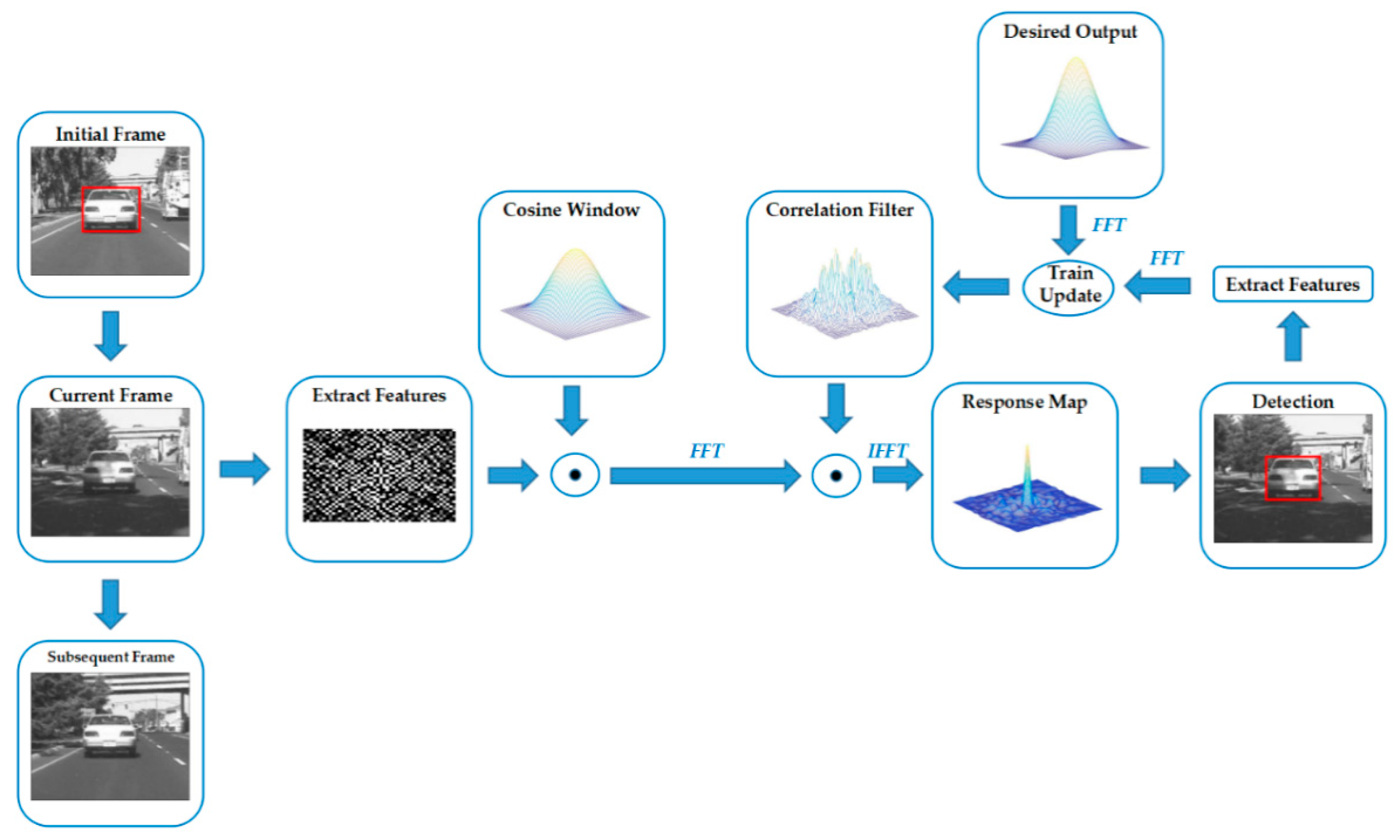
Figure 1.
Illustration of the standard DCF framework. Firstly, the correlation filter is trained by the first frame with an initial bounding box and the desired output. Secondly, it extracts the features from the current frame and multiplies a cosine window to emphasis on the center region. The features are then transformed into the frequency domain by utilizing the fast Fourier transformation (FFT). Thirdly, the response map is obtained by multiplying the correlation filter and the extracted features. The response map is transformed into the time domain by applying the inverse fast Fourier transformation (IFFT). Finally, the position of the maximum value of the response map is regarded as the center position of the target in the current frame. The new features are then extracted from the detected result to train and update the correlation filter.
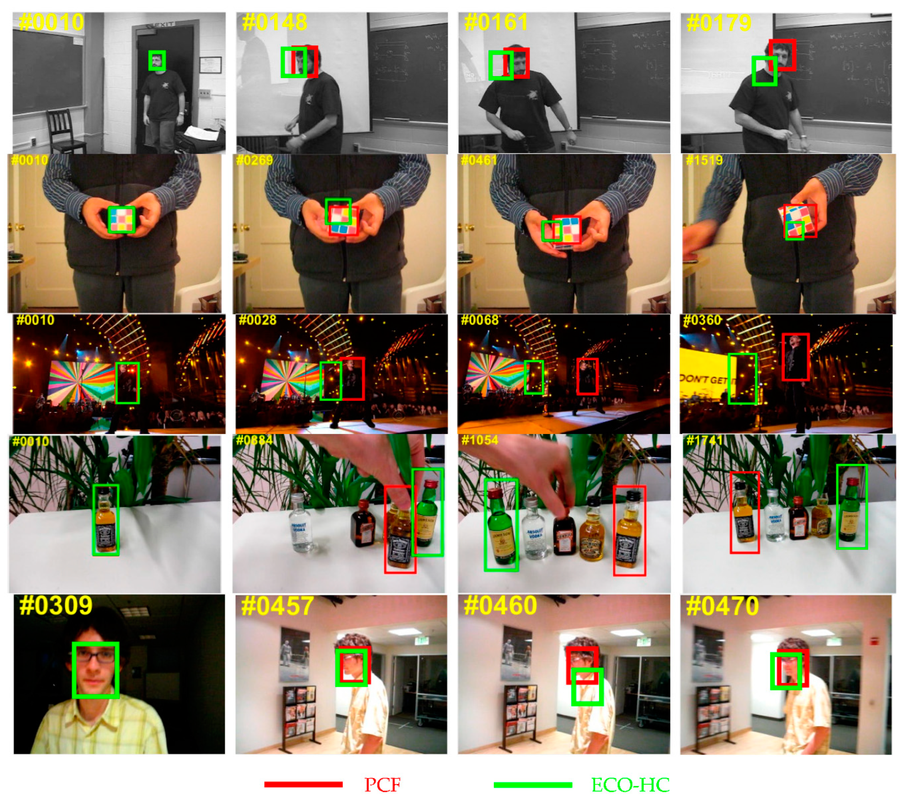
Figure 2.
The qualitative comparisons of the proposed parallel correlation filters (PCF) tracker with the baseline tracker efficient convolution operators with hand-crafted features (ECO-HC) on five challenging sequences of the benchmarks. The results are marked in different colors. On all these five cases, PCF tracker performs better center position precision and overlap precision than the baseline tracker. PCF tracker successfully tracks the target when the target undergoes significant rotation, illumination variation, and deformation.
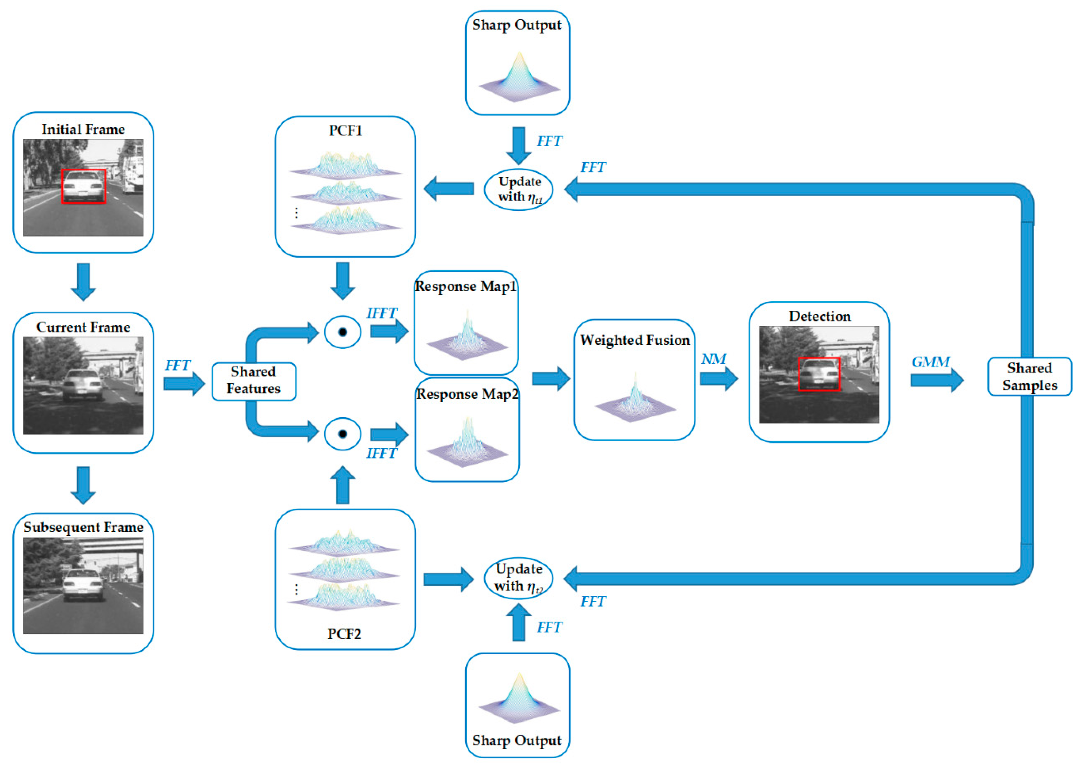
Figure 3.
The flow chart of the proposed PCF framework. In the initial frame, the PCF tracker trains two parallel correlation filters PCF1 and PCF2 online in the frequency domain utilizing the shared samples and the sharp correlation output. In the current frame, PCF1 and PCF2 are utilized to track the target respectively. Through weighting the response maps of PCF1 and PCF2, the PCF tracker accurately detects the position of the target by applying the Newton method (NM). It then utilizes the Gaussian mixture model (GMM) to generate a new shared sample set by adding a new sample or merging the two closest samples. It utilizes the new sample set to update the two parallel correlation filters with different learning rates every six frames.
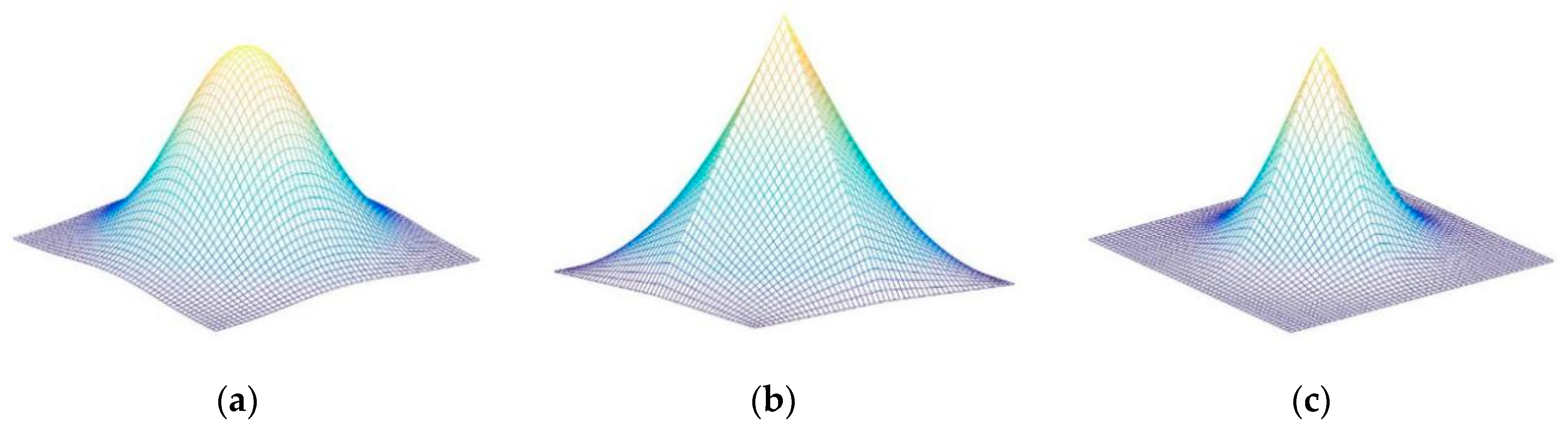
Figure 4.
Different distributions of the desired correlation output: (a) 2-D Gaussian distribution; (b) 2-D triangle distribution; (c) 2-D merged distribution.
Figure 4.
Different distributions of the desired correlation output: (a) 2-D Gaussian distribution; (b) 2-D triangle distribution; (c) 2-D merged distribution.
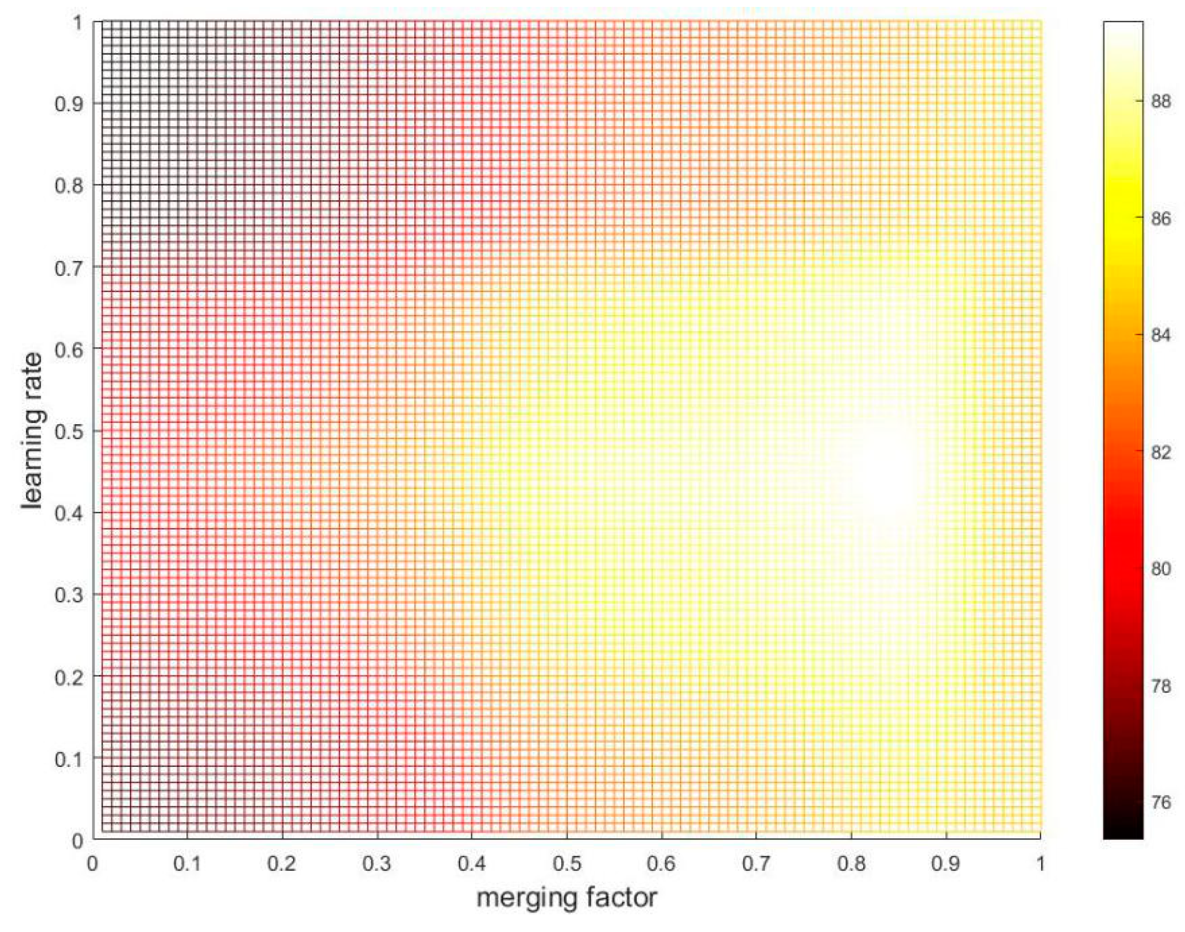
Figure 5.
The results of the parameter setting experiments on OTB-2013 benchmark. The color bar denotes the one pass evaluation (OPE) accuracy percent (%) of location error threshold (LET) at 20 pixels. The horizontal and vertical coordinates represent merging factor and learning rate respectively. The points ranging from (0.1, 0.1), (0.1, 0.2), …, (1.0, 1.0) were obtained in experiments, others were obtained by the linear interpolation method. When the point is set to (0.9, 0.5), the OPE accuracy is maximized.
Figure 6.
The results of the ablation experiments on OTB-2013 benchmark for the baseline tracker, the proposed PCF tracker and the trackers of progressively integrating the presented strategies: (a) The precision plots (PP) of one pass evaluation (OPE) and the values in brackets denote the OPE accuracy of location error threshold (LET) at 20 pixels; (b) The success plots (SP) of the OPE and the numbers in brackets are the areas under the curve (AUC).
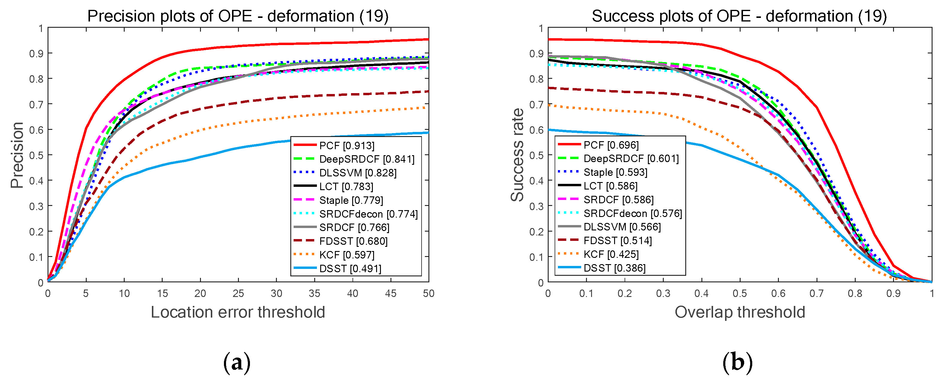
Figure 7.
The quantitative results of the top ten trackers on OTB-2013 benchmark among three different contributions: DEF, OPR, and IV. Among the top ten trackers, the proposed PCF tracker obtains the best results on all three attributes: (a) The PP of the OPE on attribute DEF; (b) The SP of the OPE on attribute DEF; (c) The PP of the OPE on attribute OPR; (d) The SP of the OPE on attribute OPR; (e) The PP of OPE on attribute IV; (f) The SP of the OPE on attribute IV.
Figure 8.
The comparing results for the top ten trackers with the whole 50 sequences on OTB-2013 benchmark: (a) The PP of the OPE on all sequences; (b) The SP of the OPE on all sequences.
Figure 8.
The comparing results for the top ten trackers with the whole 50 sequences on OTB-2013 benchmark: (a) The PP of the OPE on all sequences; (b) The SP of the OPE on all sequences.
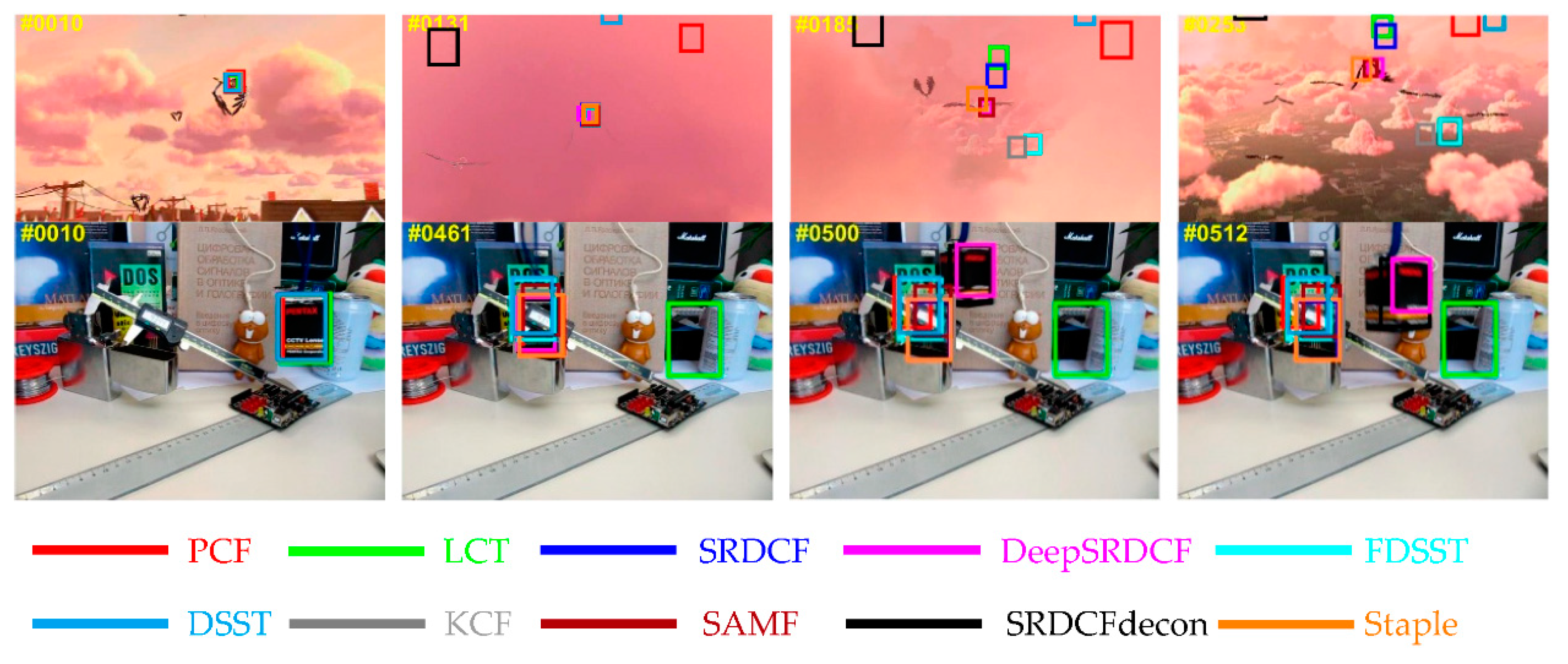
Figure 9.
The qualitative experiments from four representative sequences on the OTB-2013 benchmark. The results for the top ten trackers are expressed in different colors. On these challenging sequences, the proposed PCF tracker achieves remarkable results compared to the other top nine trackers in terms of accuracy and robustness.
Figure 10.
The quantitative results of the top ten trackers on OTB-2015 benchmark determined by three challenge contributions: DEF, OPR, and IV. Among the top ten trackers, the proposed PCF tracker achieves the top ranks in all three attributes: (a) The PP of the OPE on attribute DEF; (b) The SP of the OPE on attribute DEF; (c) The PP of the OPE on attribute OPR; (d) The SP of the OPE on attribute OPR; (e) The PP of the OPE on attribute IV; (f) The SP of the OPE on attribute IV.
Figure 11.
The comparing results for the top ten trackers with the entire 100 videos on the OTB-2015 benchmark: (a) The PP of the OPE on all videos; (b) The SP of the OPE on all videos.
Figure 11.
The comparing results for the top ten trackers with the entire 100 videos on the OTB-2015 benchmark: (a) The PP of the OPE on all videos; (b) The SP of the OPE on all videos.
Figure 12.
The qualitative experiments from four representative videos on the OTB-2015 benchmark. The results for the top ten trackers are marked in different colors. In these challenging videos, the proposed PCF tracker performs better than the other top nine trackers.
Figure 12.
The qualitative experiments from four representative videos on the OTB-2015 benchmark. The results for the top ten trackers are marked in different colors. In these challenging videos, the proposed PCF tracker performs better than the other top nine trackers.
Figure 13.
The failure cases from two representative sequences on the benchmarks. The tracking results for the top ten trackers are marked in different colors.
Figure 13.
The failure cases from two representative sequences on the benchmarks. The tracking results for the top ten trackers are marked in different colors.
Table 1.
The parameter settings of the proposed PCF tracker.
Table 1.
The parameter settings of the proposed PCF tracker.
| Parameters | | | | | |
|---|
| Values | 0.009 | 0.5 | 0.9 | 1.0 | 30 |
Table 2.
The PP of the OPE for the baseline tracker, the proposed PCF tracker and the trackers of progressively integrating the presented strategies on eleven different attributes (the ranks of results are expressed in %): scale variation (SV), illumination variation (IV), out-of-plane rotation (OPR), occlusion (OCC), background cluttered (BC), deformation (DEF), motion blur (MB), fast motion (FM), in-plane rotation (IPR), out-of-view (OV), and low resolution (LR). The last column is the average running speed (FPS) on all sequences of OTB-2013. The top three ranks are marked in red, cyan, and blue respectively.
| Trackers | SV | IV | OPR | OCC | BC | DEF | MB | FM | IPR | OV | LR | Speed |
|---|
| Baseline | 78.2 | 77.3 | 82.9 | 86.1 | 77.7 | 86.1 | 71.6 | 74.3 | 77.5 | 74.7 | 56.5 | 49 |
| PCF_WF | 80.3 | 80.9 | 87.2 | 89.1 | 82.4 | 91.2 | 73.9 | 74.3 | 81.3 | 79.7 | 71.0 | 44 |
| PCF_SR | 83.5 | 79.4 | 87.0 | 91.0 | 81.3 | 86.2 | 74.7 | 78.0 | 80.9 | 81.9 | 76.7 | 47 |
| PCF | 82.4 | 82.1 | 88.4 | 89.5 | 84.5 | 91.3 | 76.0 | 76.7 | 82.7 | 81.1 | 73.3 | 42 |
Table 3.
The SP of the OPE for the baseline tracker, the proposed PCF tracker and the trackers of progressively integrating the presented strategies on different attributes (%): SV, IV, OPR, OCC, BC, DEF, MB, FM, IPR, OV, LR. The last column is the AUC which represents the average overlap accuracy of the OPE. The top three ranks are marked in red, cyan, and blue separately.
| Trackers | SV | IV | OPR | OCC | BC | DEF | MB | FM | IPR | OV | LR | AUC |
|---|
| Baseline | 60.3 | 59.5 | 61.6 | 64.4 | 58.5 | 65.1 | 57.7 | 57.8 | 58.1 | 60.1 | 35.8 | 64.3 |
| PCF_WF | 61.2 | 61.8 | 64.5 | 65.9 | 61.0 | 68.9 | 58.1 | 57.5 | 60.4 | 63.4 | 44.5 | 66.2 |
| PCF_SR | 62.8 | 60.4 | 64.2 | 67.4 | 60.3 | 65.6 | 58.3 | 59.0 | 59.6 | 64.7 | 48.1 | 66.0 |
| PCF | 63.2 | 63.1 | 65.9 | 66.9 | 63.5 | 69.6 | 60.1 | 59.3 | 62.2 | 64.5 | 48.8 | 67.5 |
Table 4.
The PP of the OPE on OTB-2013 benchmark for the top ten trackers on eleven different attributes (%): SV, IV, OPR, OCC, BC, DEF, MB, FM, IPR, OV, LR. The last column is the average precision (AP) of LET at 20 pixels. The top three ranks are marked in red, cyan, and blue, respectively.
Table 4.
The PP of the OPE on OTB-2013 benchmark for the top ten trackers on eleven different attributes (%): SV, IV, OPR, OCC, BC, DEF, MB, FM, IPR, OV, LR. The last column is the average precision (AP) of LET at 20 pixels. The top three ranks are marked in red, cyan, and blue, respectively.
| Trackers | SV | IV | OPR | OCC | BC | DEF | MB | FM | IPR | OV | LR | AP |
|---|
| PCF | 63.2 | 63.1 | 65.9 | 66.9 | 63.5 | 69.6 | 60.1 | 59.3 | 62.2 | 64.5 | 48.8 | 67.5 |
| DeepSRDCF | 57.5 | 53.6 | 58.6 | 59.9 | 53.6 | 60.1 | 54.2 | 54.8 | 55.0 | 56.6 | 46.1 | 60.0 |
| SiamFC_3s | 57.0 | 50.5 | 55.9 | 56.1 | 54.2 | 53.5 | 49.0 | 51.5 | 55.2 | 54.5 | 52.9 | 58.5 |
| SRDCF | 54.1 | 51.5 | 55.1 | 57.4 | 53.0 | 58.6 | 51.6 | 51.4 | 51.7 | 51.1 | 41.0 | 57.4 |
| Staple | 53.7 | 54.3 | 55.7 | 55.9 | 54.5 | 59.3 | 47.8 | 45.2 | 53.5 | 40.5 | 36.2 | 56.1 |
| SAMF | 49.2 | 49.2 | 52.5 | 56.6 | 49.8 | 54.9 | 49.8 | 47.9 | 50.9 | 57.1 | 33.8 | 54.1 |
| LCT | 50.4 | 49.3 | 53.8 | 52.0 | 53.9 | 58.6 | 42.3 | 40.8 | 51.4 | 48.4 | 34.8 | 54.1 |
| FDSST | 52.1 | 51.7 | 52.1 | 50.7 | 57.3 | 51.4 | 48.8 | 47.5 | 52.3 | 47.9 | 28.8 | 54.0 |
| DLSSVM | 42.0 | 45.9 | 49.9 | 51.2 | 49.8 | 56.6 | 52.4 | 48.9 | 48.9 | 49.3 | 35.9 | 51.5 |
| DSST | 47.6 | 44.6 | 43.1 | 44.9 | 45.8 | 38.6 | 34.3 | 34.5 | 46.1 | 38.4 | 31.3 | 46.9 |
Table 5.
The SP of the OPE on OTB-2013 benchmark for the top ten trackers on eleven different attributes (%): SV, IV, OPR, OCC, BC, DEF, MB, FM, IPR, OV, LR. The last column is the average overlap accuracy of the OPE. The top three ranks are marked in red, cyan, and blue respectively.
Table 5.
The SP of the OPE on OTB-2013 benchmark for the top ten trackers on eleven different attributes (%): SV, IV, OPR, OCC, BC, DEF, MB, FM, IPR, OV, LR. The last column is the average overlap accuracy of the OPE. The top three ranks are marked in red, cyan, and blue respectively.
| Trackers | SV | IV | OPR | OCC | BC | DEF | MB | FM | IPR | OV | LR | AUC |
|---|
| PCF | 82.4 | 82.1 | 88.4 | 89.5 | 84.5 | 91.3 | 76.0 | 76.7 | 82.7 | 81.1 | 73.3 | 89.2 |
| DeepSRDCF | 80.7 | 76.5 | 84.6 | 85.9 | 76.7 | 84.1 | 74.9 | 75.6 | 80.0 | 78.2 | 74.9 | 85.3 |
| SiamFC_3s | 76.7 | 68.0 | 76.3 | 75.6 | 73.1 | 70.9 | 64.7 | 68.2 | 74.7 | 68.3 | 78.0 | 79.3 |
| SRDCF | 75.9 | 69.0 | 76.5 | 77.2 | 70.6 | 76.6 | 69.8 | 69.4 | 72.2 | 65.4 | 76.8 | 78.9 |
| Staple | 75.3 | 73.5 | 77.0 | 76.3 | 73.8 | 77.9 | 62.7 | 60.4 | 73.4 | 65.4 | 72.2 | 76.5 |
| SAMF | 73.4 | 69.0 | 75.9 | 80.7 | 65.6 | 74.0 | 64.8 | 63.0 | 72.9 | 66.8 | 70.8 | 77.4 |
| LCT | 72.1 | 68.6 | 76.0 | 71.1 | 73.5 | 78.3 | 55.9 | 52.0 | 72.4 | 56.7 | 68.1 | 75.9 |
| FDSST | 75.1 | 74.0 | 74.2 | 70.7 | 79.4 | 68.0 | 68.3 | 64.4 | 74.0 | 59.6 | 53.9 | 75.3 |
| DLSSVM | 67.4 | 66.5 | 75.6 | 72.3 | 69.6 | 82.8 | 72.9 | 66.8 | 74.2 | 61.9 | 82.6 | 75.7 |
| DSST | 68.2 | 60.0 | 60.0 | 60.1 | 59.8 | 49.1 | 43.2 | 42.1 | 65.1 | 48.6 | 69.3 | 64.3 |
Table 6.
The PP of the OPE on the OTB-2015 benchmark for the top ten trackers on eleven different attributes (%): SV, IV, OPR, OCC, BC, DEF, MB, FM, IPR, OV, LR. The last column is the AP of LET at 20 pixels. The top three ranks are expressed in red, cyan, and blue respectively.
Table 6.
The PP of the OPE on the OTB-2015 benchmark for the top ten trackers on eleven different attributes (%): SV, IV, OPR, OCC, BC, DEF, MB, FM, IPR, OV, LR. The last column is the AP of LET at 20 pixels. The top three ranks are expressed in red, cyan, and blue respectively.
| Trackers | SV | IV | OPR | OCC | BC | DEF | MB | FM | IPR | OV | LR | AP |
|---|
| PCF | 83.9 | 82.5 | 85.1 | 84.4 | 82.8 | 83.0 | 82.3 | 82.4 | 80.7 | 79.1 | 89.2 | 86.3 |
| DeepSRDCF | 80.8 | 80.0 | 82.9 | 83.4 | 78.7 | 78.7 | 79.4 | 79.3 | 81.9 | 81.1 | 88.0 | 84.2 |
| SRDCFdecon | 75.6 | 76.2 | 72.8 | 71.5 | 74.2 | 72.4 | 74.2 | 72.1 | 71.3 | 59.6 | 78.2 | 77.3 |
| SRDCF | 71.8 | 73.4 | 69.9 | 66.7 | 68.0 | 68.2 | 70.0 | 71.1 | 71.7 | 55.0 | 79.5 | 75.3 |
| Staple | 73.2 | 76.4 | 72.6 | 69.9 | 71.4 | 71.0 | 64.9 | 67.7 | 75.7 | 59.2 | 77.3 | 75.0 |
| SAMF | 68.4 | 70.1 | 71.0 | 69.8 | 63.6 | 67.4 | 59.8 | 65.0 | 71.9 | 57.3 | 76.9 | 73.5 |
| LCT | 63.5 | 73.2 | 69.3 | 61.0 | 66.5 | 65.5 | 55.2 | 57.5 | 70.8 | 44.1 | 68.4 | 70.1 |
| FDSST | 64.1 | 70.9 | 62.6 | 59.9 | 74.5 | 57.1 | 63.8 | 65.6 | 69.2 | 52.5 | 65.3 | 68.7 |
| DSST | 61.8 | 62.1 | 57.1 | 53.7 | 62.2 | 49.7 | 51.4 | 51.9 | 64.1 | 50.1 | 68.8 | 63.3 |
| KCF | 58.0 | 63.1 | 59.6 | 52.6 | 62.3 | 55.9 | 50.6 | 54.9 | 63.5 | 37.2 | 67.1 | 62.3 |
Table 7.
SP of the OPE on OTB-2015 benchmark for the top ten trackers on eleven different attributes (%): SV, IV, OPR, OCC, BC, DEF, MB, FM, IPR, OV, LR. The last column is the average precision of LET at 20 pixels. The last column is the AUC of the OPE. The top three ranks are expressed in red, cyan, and blue respectively.
| Trackers | SV | IV | OPR | OCC | BC | DEF | MB | FM | IPR | OV | LR | AUC |
|---|
| PCF | 61.6 | 63.6 | 62.6 | 61.6 | 63.0 | 62.5 | 63.2 | 61.4 | 59.3 | 56.2 | 56.0 | 64.7 |
| DeepSRDCF | 56.5 | 57.0 | 56.8 | 57.5 | 55.7 | 53.6 | 58.9 | 57.8 | 54.6 | 54.1 | 50.5 | 58.7 |
| SRDCFdecon | 54.3 | 55.7 | 52.1 | 52.7 | 55.0 | 52.2 | 57.2 | 54.5 | 49.9 | 48.0 | 46.7 | 55.9 |
| SRDCF | 51.8 | 54.2 | 50.6 | 50.7 | 51.4 | 50.4 | 52.9 | 54.4 | 50.0 | 42.8 | 46.8 | 54.7 |
| Staple | 51.3 | 55.4 | 51.6 | 51.3 | 52.3 | 52.3 | 50.4 | 50.7 | 51.4 | 45.0 | 41.1 | 53.7 |
| SAMF | 46.0 | 49.2 | 49.3 | 48.9 | 47.5 | 46.9 | 47.3 | 48.9 | 48.9 | 44.8 | 39.3 | 51.0 |
| FDSST | 46.4 | 49.6 | 45.7 | 44.3 | 54.2 | 42.8 | 47.6 | 49.6 | 49.6 | 41.5 | 39.1 | 50.0 |
| LCT | 44.7 | 50.0 | 48.8 | 45.0 | 49.5 | 46.7 | 44.2 | 45.7 | 48.3 | 37.8 | 37.1 | 49.9 |
| DSST | 43.3 | 45.1 | 41.2 | 40.4 | 46.1 | 37.2 | 41.0 | 41.6 | 44.7 | 39.0 | 33.8 | 45.6 |
| KCF | 36.4 | 41.0 | 39.6 | 36.8 | 43.4 | 39.3 | 38.2 | 40.4 | 42.2 | 31.8 | 29.0 | 42.1 |


