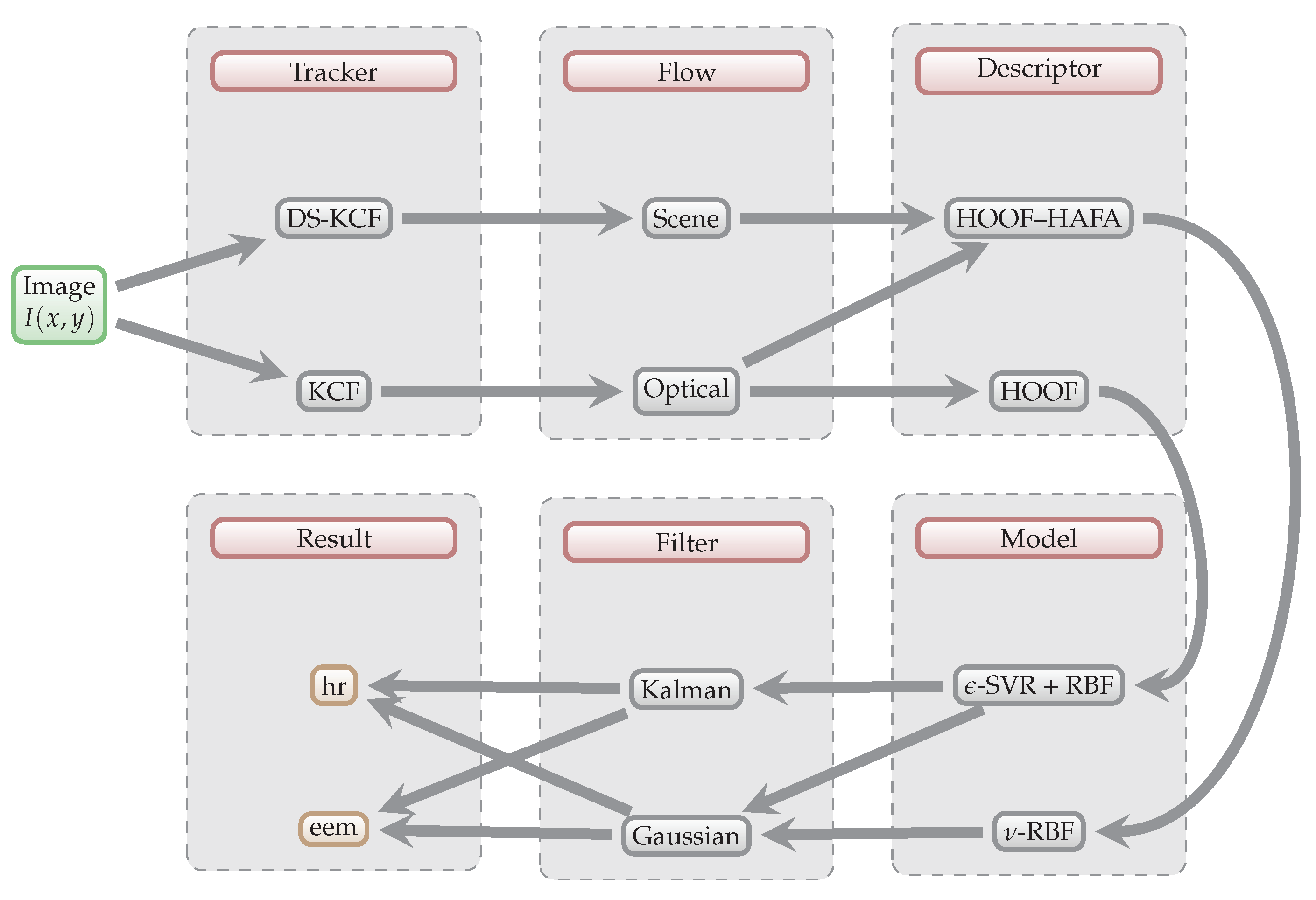
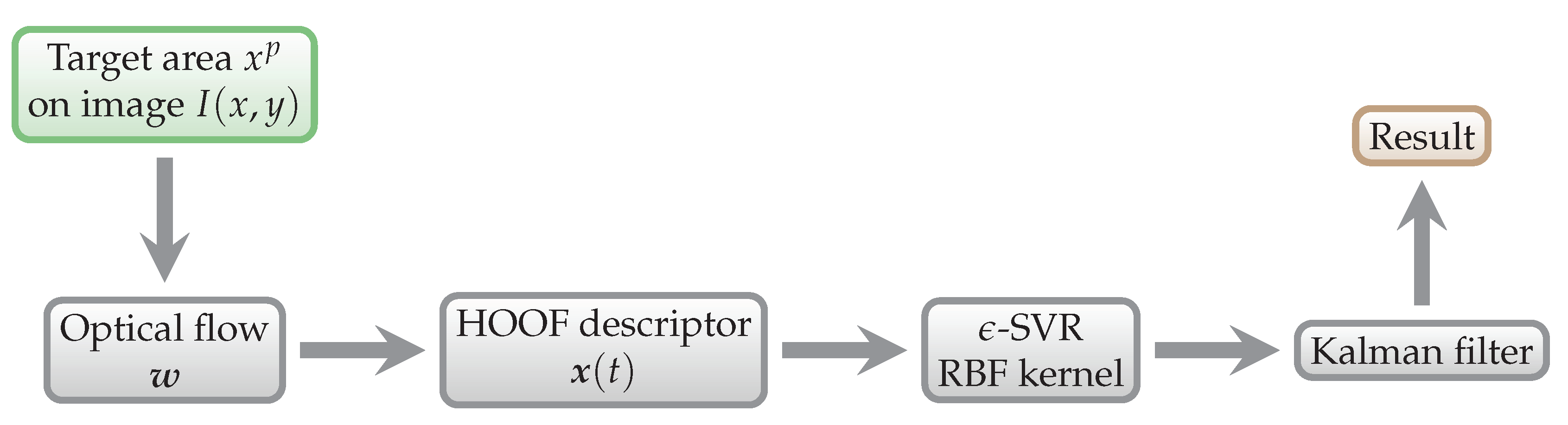
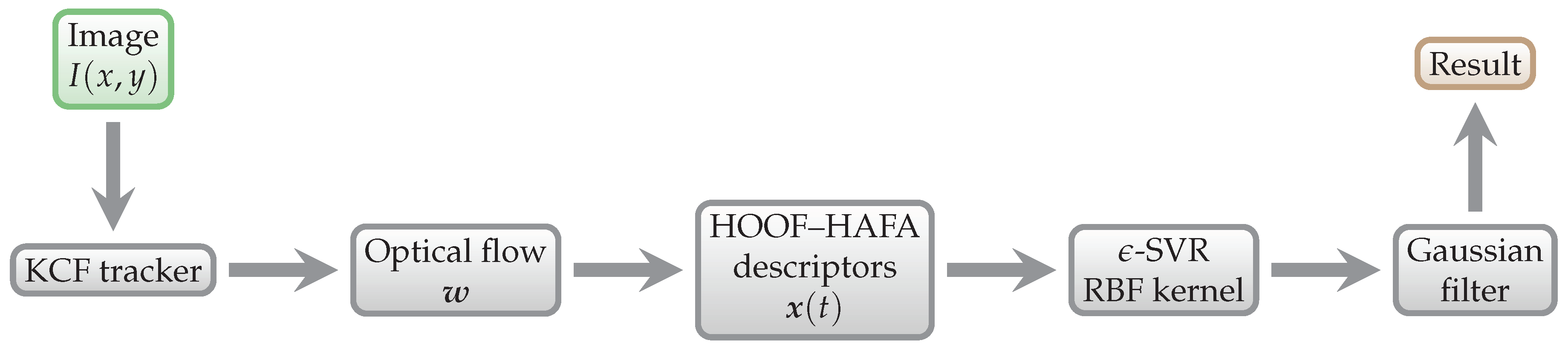
Figure 1.
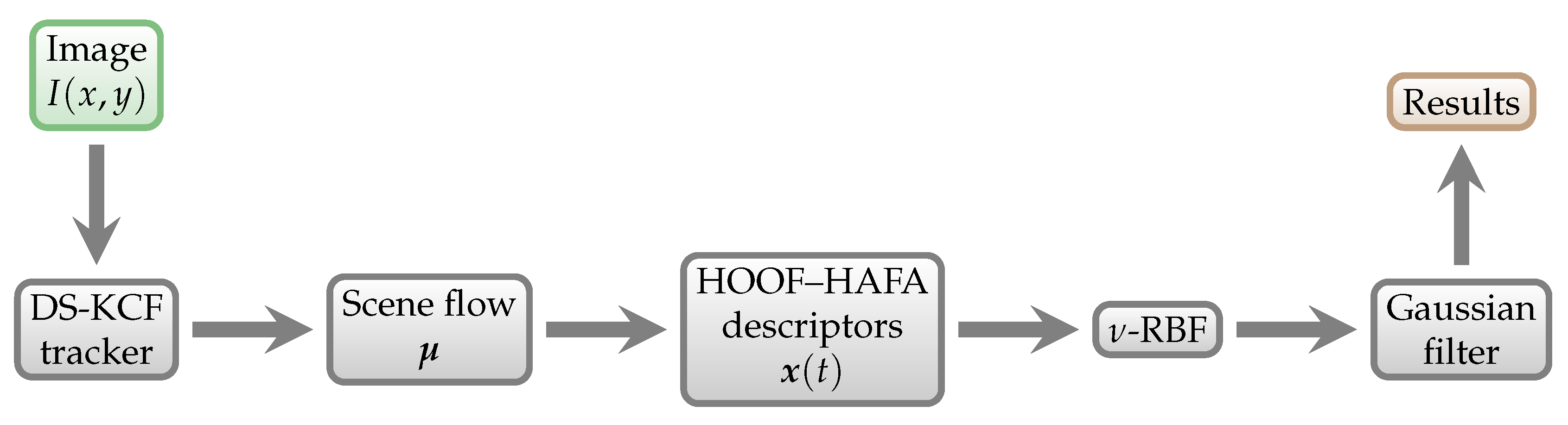
Schematic overview of our approach. Individual algorithms and methods are explained in detail in
Section 3.
Figure 1.
Schematic overview of our approach. Individual algorithms and methods are explained in detail in
Section 3.
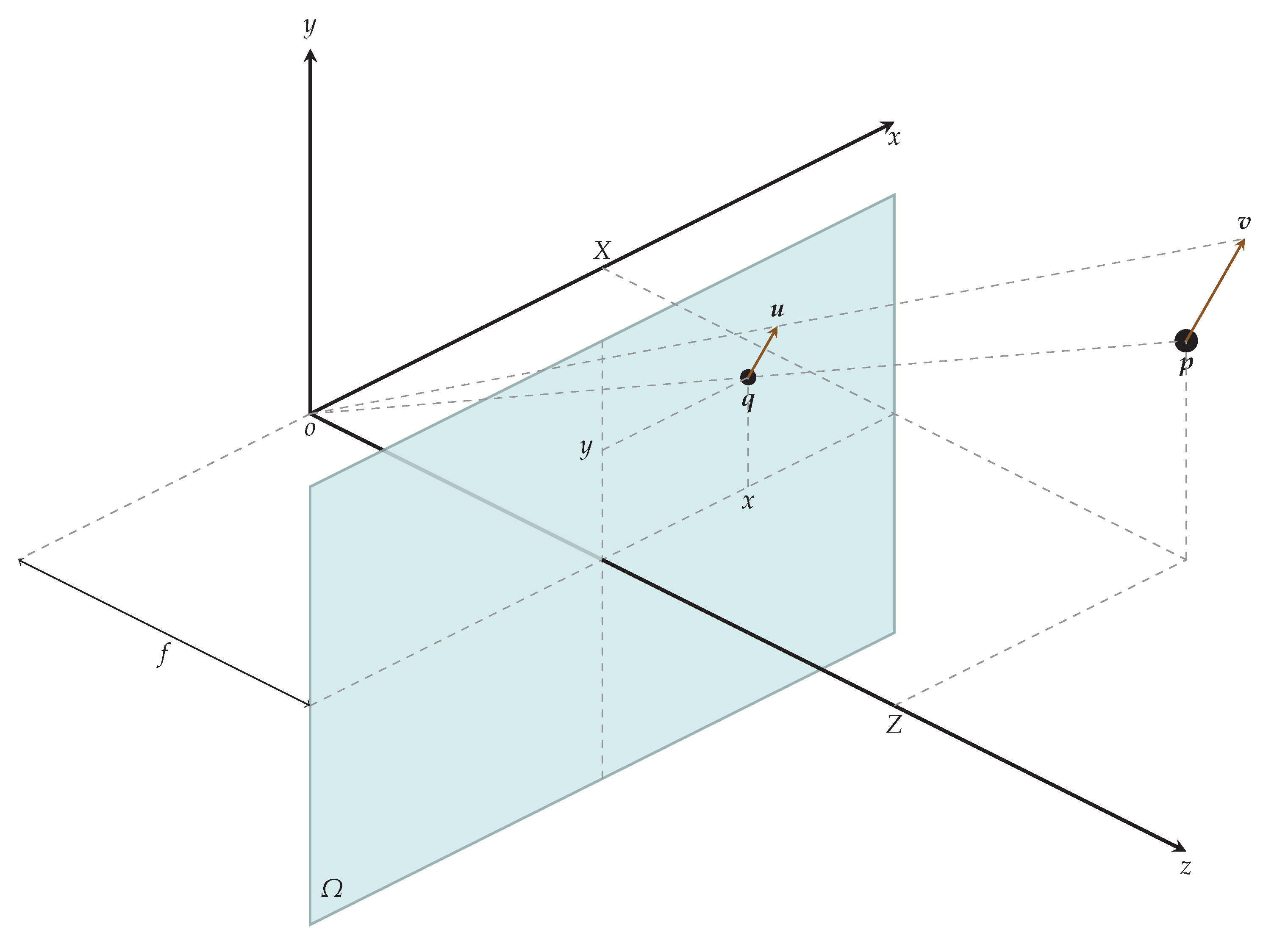
Figure 2.
Projection of velocity field onto image plane results in optical flow . In the camera coordinate system, a particle with velocity field vector has an image with motion field vector on an image plane . In reality, we can only get an approximation to motion field vector which is optical flow vector .
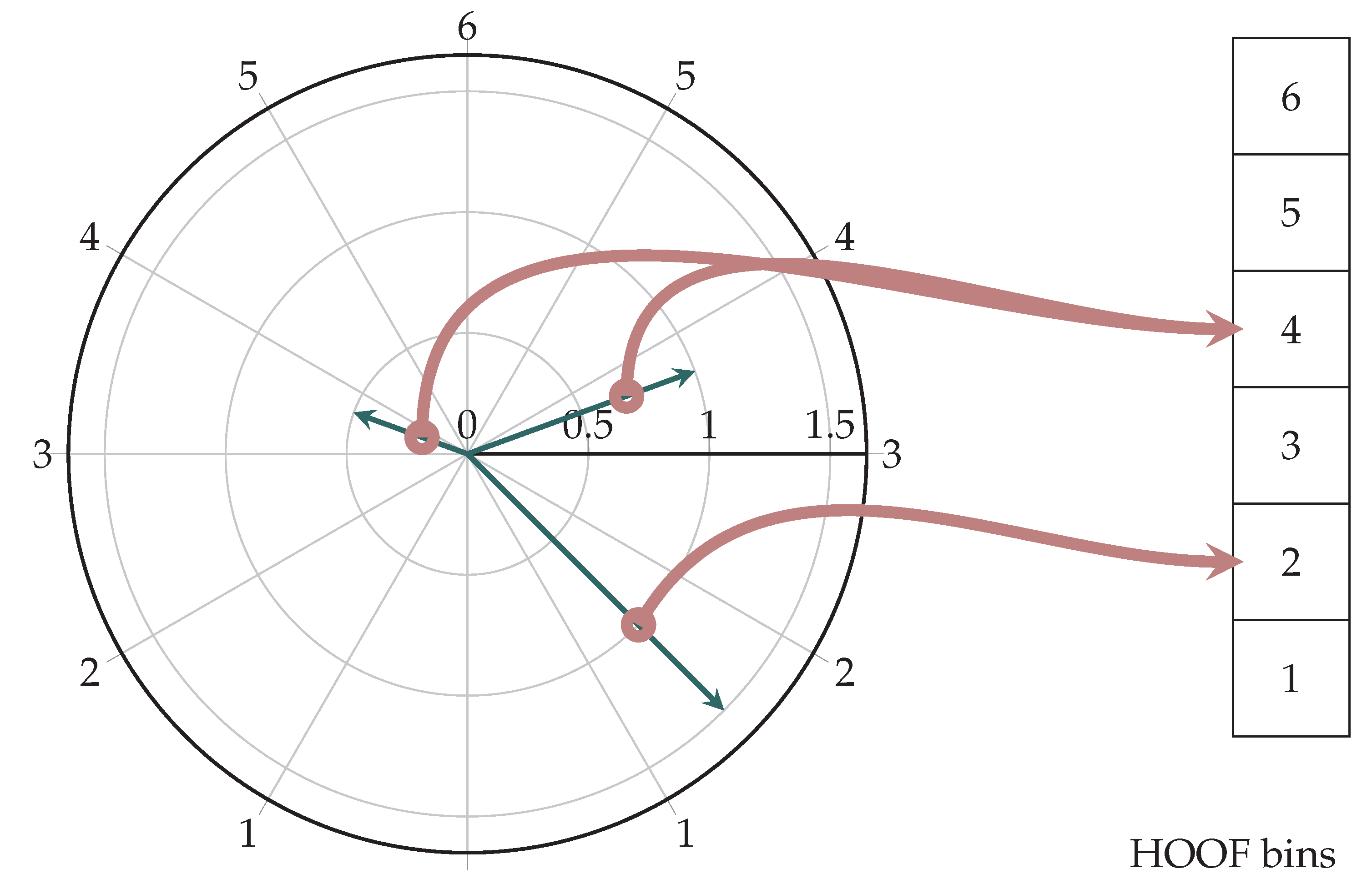
Figure 3.
Example: Calculating a six-bin HOOF histogram. Note the invariance in the direction along the x axis—this is intentional.
Figure 3.
Example: Calculating a six-bin HOOF histogram. Note the invariance in the direction along the x axis—this is intentional.
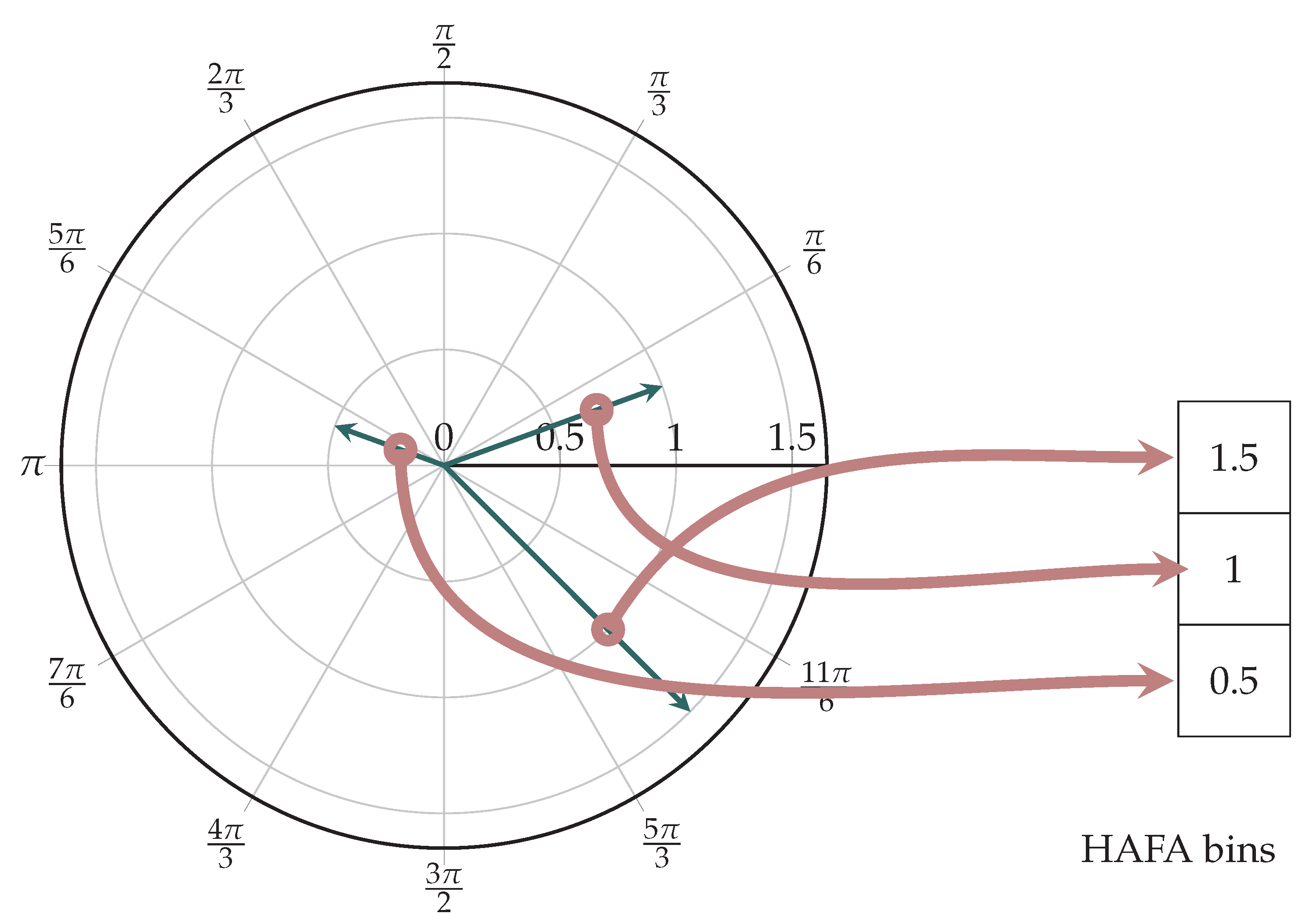
Figure 4.
Example: Calculating a three-bin HAFA histogram.
Figure 4.
Example: Calculating a three-bin HAFA histogram.
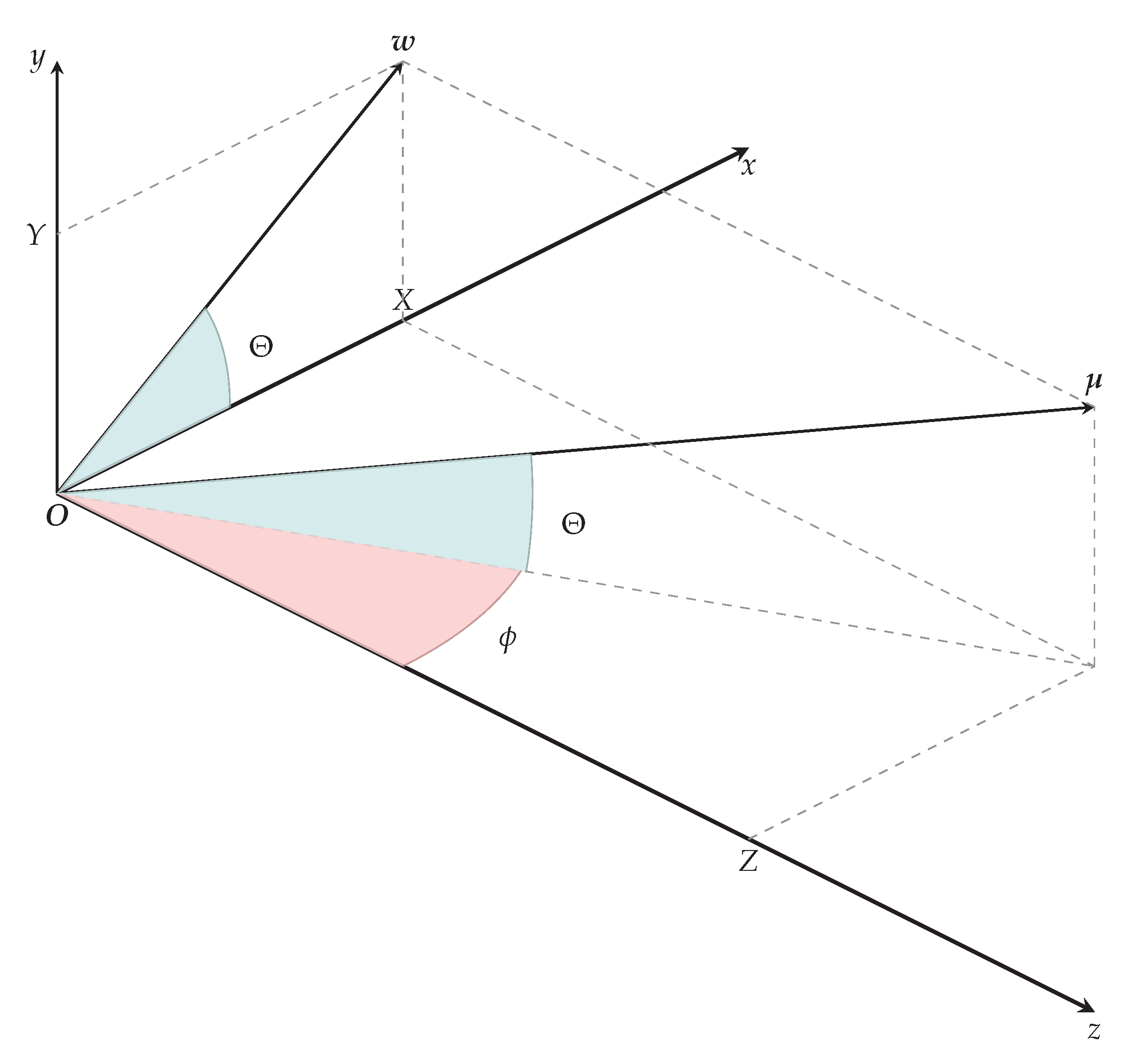
Figure 5.
Spherical coordinates in camera coordinate system help us to extend histogram descriptors for use with the scene flow.
Figure 5.
Spherical coordinates in camera coordinate system help us to extend histogram descriptors for use with the scene flow.
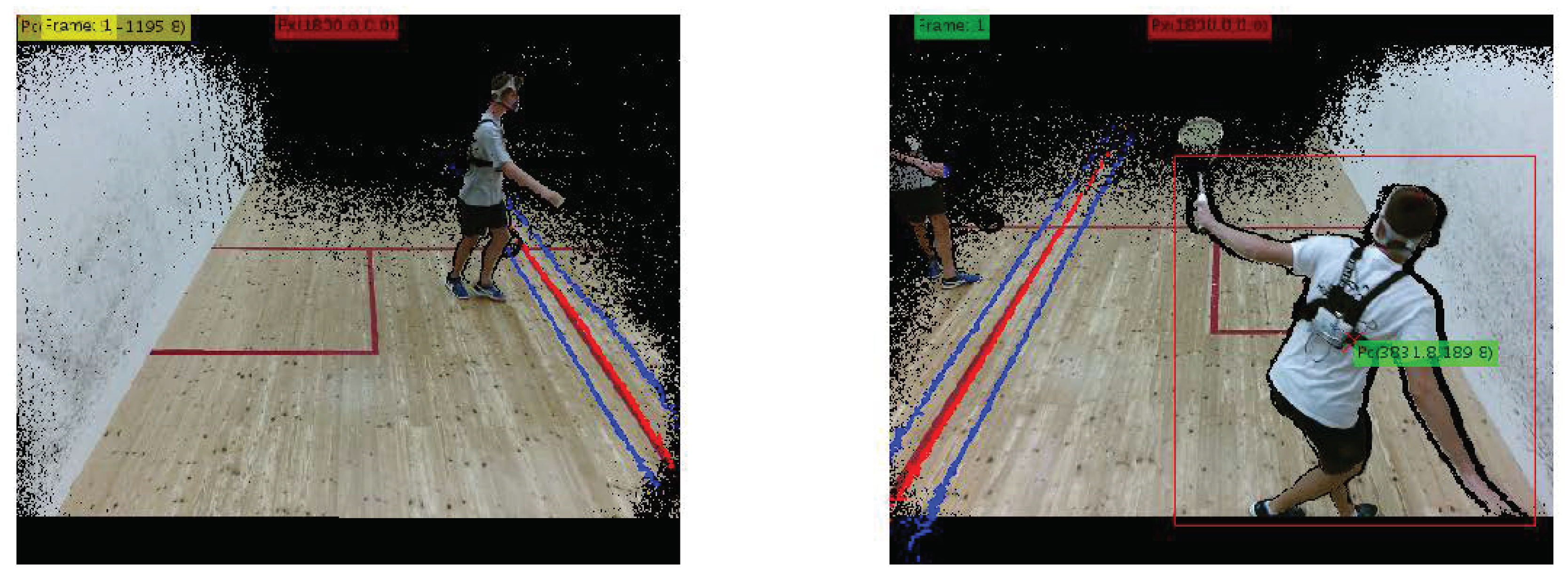
Figure 6.
Determining the intersection of visible fields of view in left and right Kinect camera. First frames of the first set in second phase of the field experiments are shown. The fourth player is marked. The green color represents the selected camera. The intersection is a red line. Blue lines are hysteresis thresholds for switching between cameras. They lie 200 mm to the left and to the right of the intersection, shown in red.
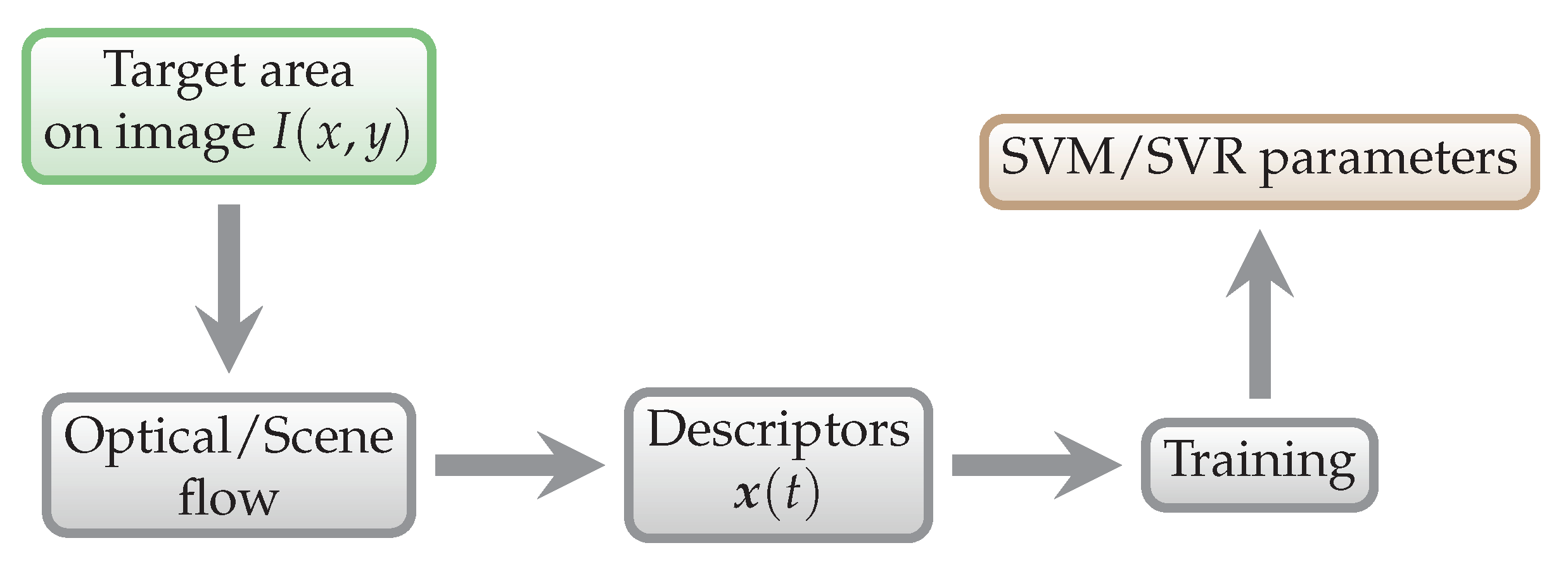
Figure 7.
General training scheme. The data that enter this process are training data.
Figure 7.
General training scheme. The data that enter this process are training data.
Figure 8.
General energy expenditure prediction scheme. The data that enter this process are testing data.
Figure 8.
General energy expenditure prediction scheme. The data that enter this process are testing data.
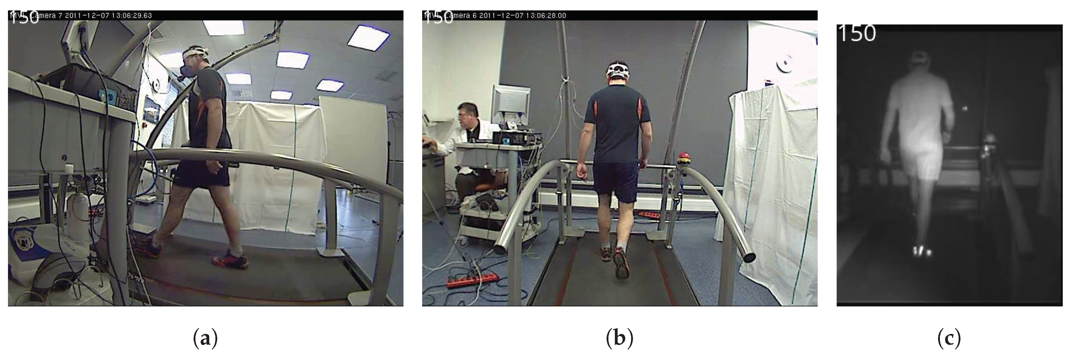
Figure 9.
Side-view back-view and NIR images of 150th frame from Phase 1 laboratory testing: (a) side-view image; (b) back-view image; and (c) NIR image.
Figure 9.
Side-view back-view and NIR images of 150th frame from Phase 1 laboratory testing: (a) side-view image; (b) back-view image; and (c) NIR image.
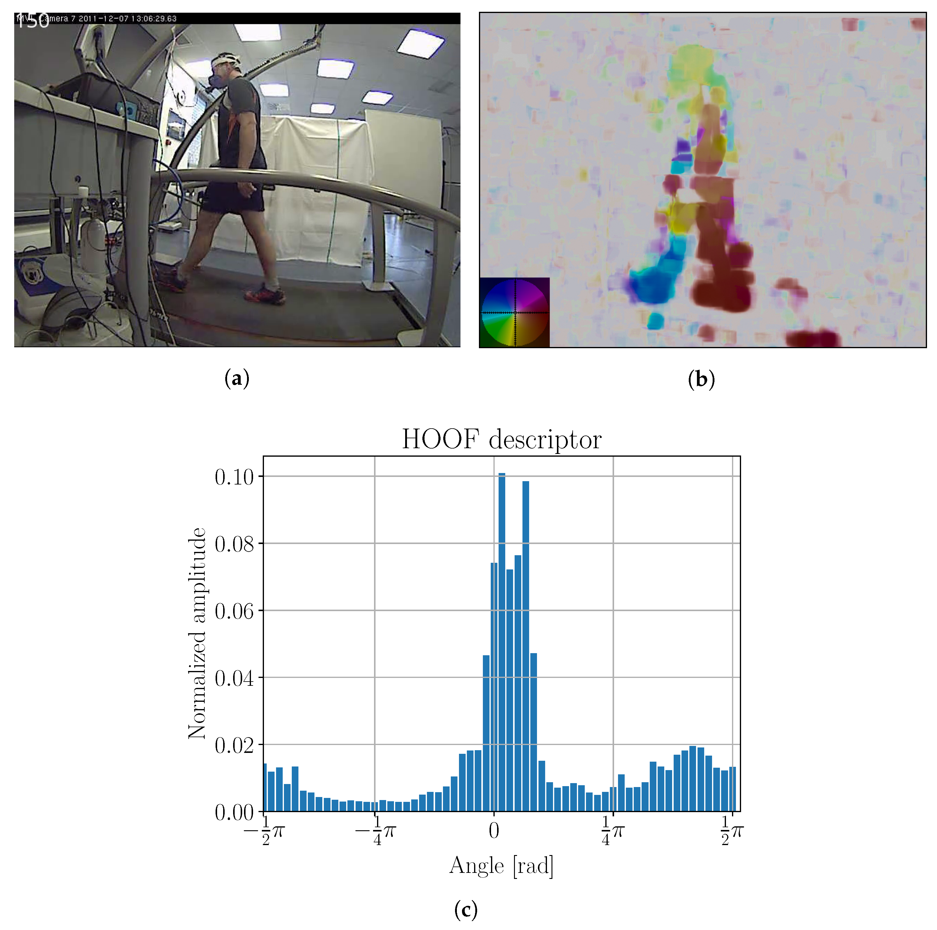
Figure 10.
(
a) Original image; (
b) optical flow; and (
c) HOOF histogram for 150th frame from Phase 1 laboratory testing. Color coding legend on the lower left in (
b) is based on [
41]. Maximal amplitude of optical flow is 17 ppf (pixels per frame).
Figure 10.
(
a) Original image; (
b) optical flow; and (
c) HOOF histogram for 150th frame from Phase 1 laboratory testing. Color coding legend on the lower left in (
b) is based on [
41]. Maximal amplitude of optical flow is 17 ppf (pixels per frame).
Figure 11.
P1OFL prediction scheme. It was used for Phase 1 lab testing.
Figure 11.
P1OFL prediction scheme. It was used for Phase 1 lab testing.
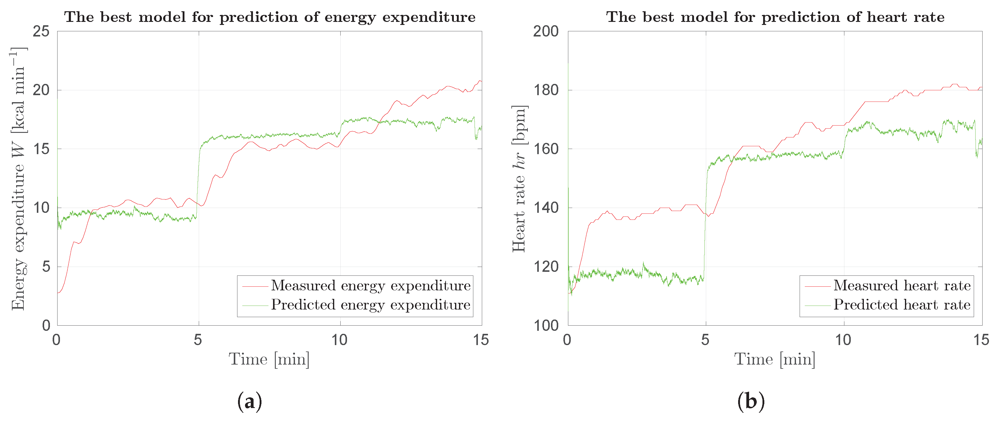
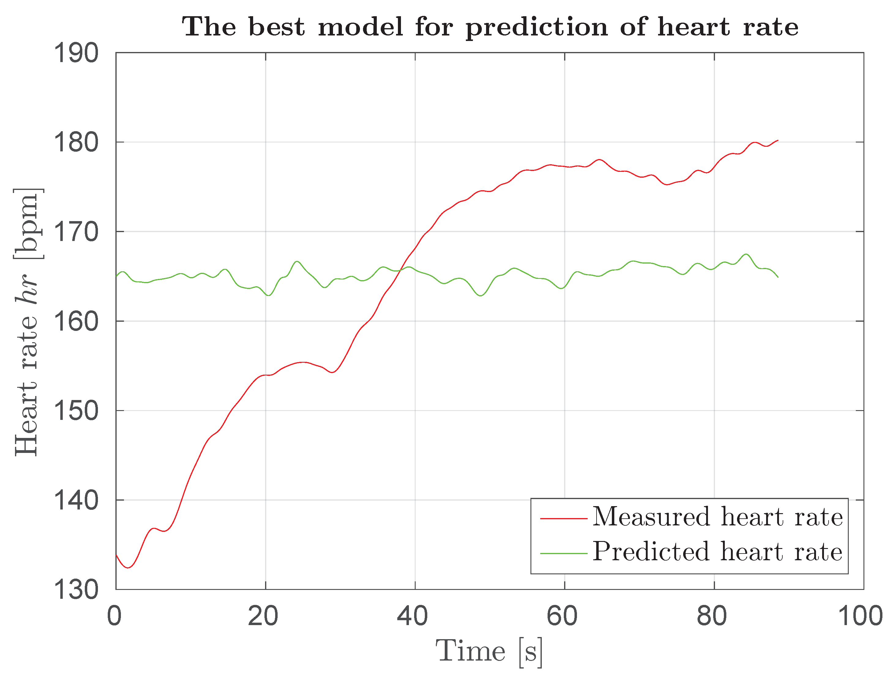
Figure 12.
The best results for prediction of energy expenditure and heart rate. Figures show output of models eem-sv(sv) and hr-sv(sv) and the actual value of energy expenditure and heart rate: (a) prediction of energy expenditure; and (b) prediction of heart rate.
Figure 12.
The best results for prediction of energy expenditure and heart rate. Figures show output of models eem-sv(sv) and hr-sv(sv) and the actual value of energy expenditure and heart rate: (a) prediction of energy expenditure; and (b) prediction of heart rate.
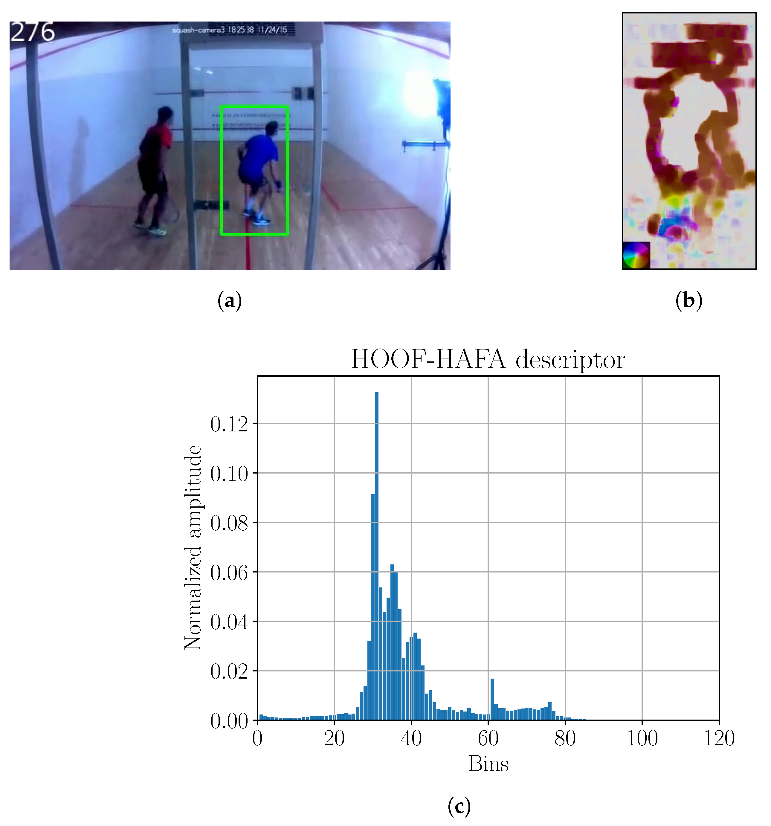
Figure 13.
(
a) Image with tracking; (
b) optical flow; (
c) HOOF–HAFA histogram. Green bounding box in sub-figure (
a) is the detection, obtained by KCF tracker. Color coding legend on the lower left in sub-figure (
b) is based on [
41]. Maximum amplitude of optical flow image is 31 ppf.
Figure 13.
(
a) Image with tracking; (
b) optical flow; (
c) HOOF–HAFA histogram. Green bounding box in sub-figure (
a) is the detection, obtained by KCF tracker. Color coding legend on the lower left in sub-figure (
b) is based on [
41]. Maximum amplitude of optical flow image is 31 ppf.
Figure 14.
P1OFC prediction scheme, used for Phase 1 field testing.
Figure 14.
P1OFC prediction scheme, used for Phase 1 field testing.
Figure 15.
Response of model hr-bv-hoofhafa(bv) for squash game.
Figure 15.
Response of model hr-bv-hoofhafa(bv) for squash game.
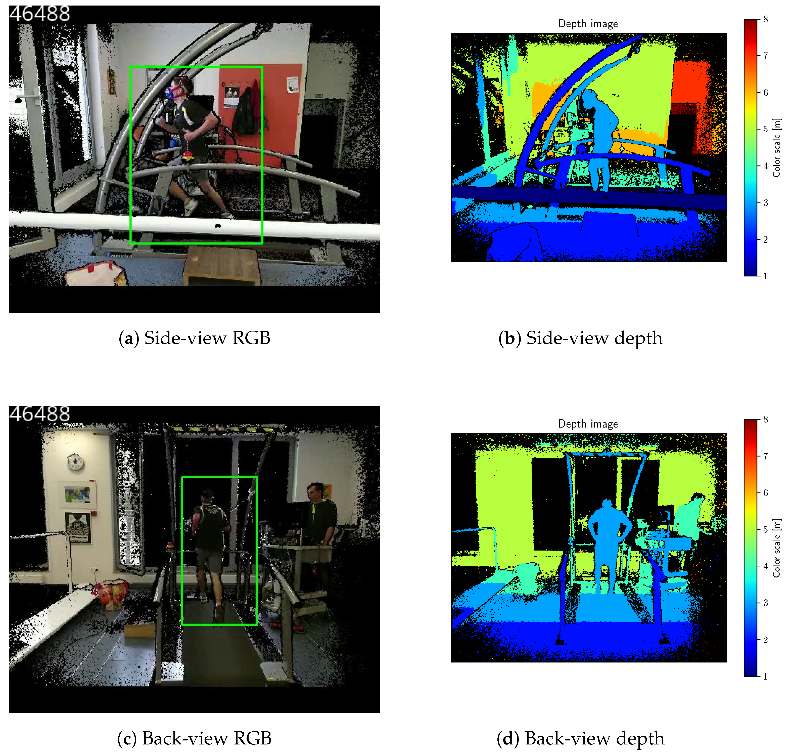
Figure 16.
Side-view and back-view images from Kinect camera in the laboratory. RGB images were registered to corresponding depth images. Black pixels do not have corresponding depth. Green bounding boxes are target detections, provided by the KCF tracker. Treadmill speed: 16 km h−1.
Figure 16.
Side-view and back-view images from Kinect camera in the laboratory. RGB images were registered to corresponding depth images. Black pixels do not have corresponding depth. Green bounding boxes are target detections, provided by the KCF tracker. Treadmill speed: 16 km h−1.
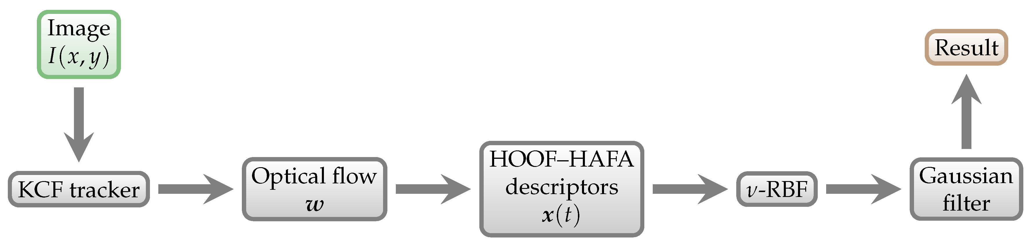
Figure 17.
P2OF prediction scheme. It is used in for Phase 2 testing with optical flow.
Figure 17.
P2OF prediction scheme. It is used in for Phase 2 testing with optical flow.
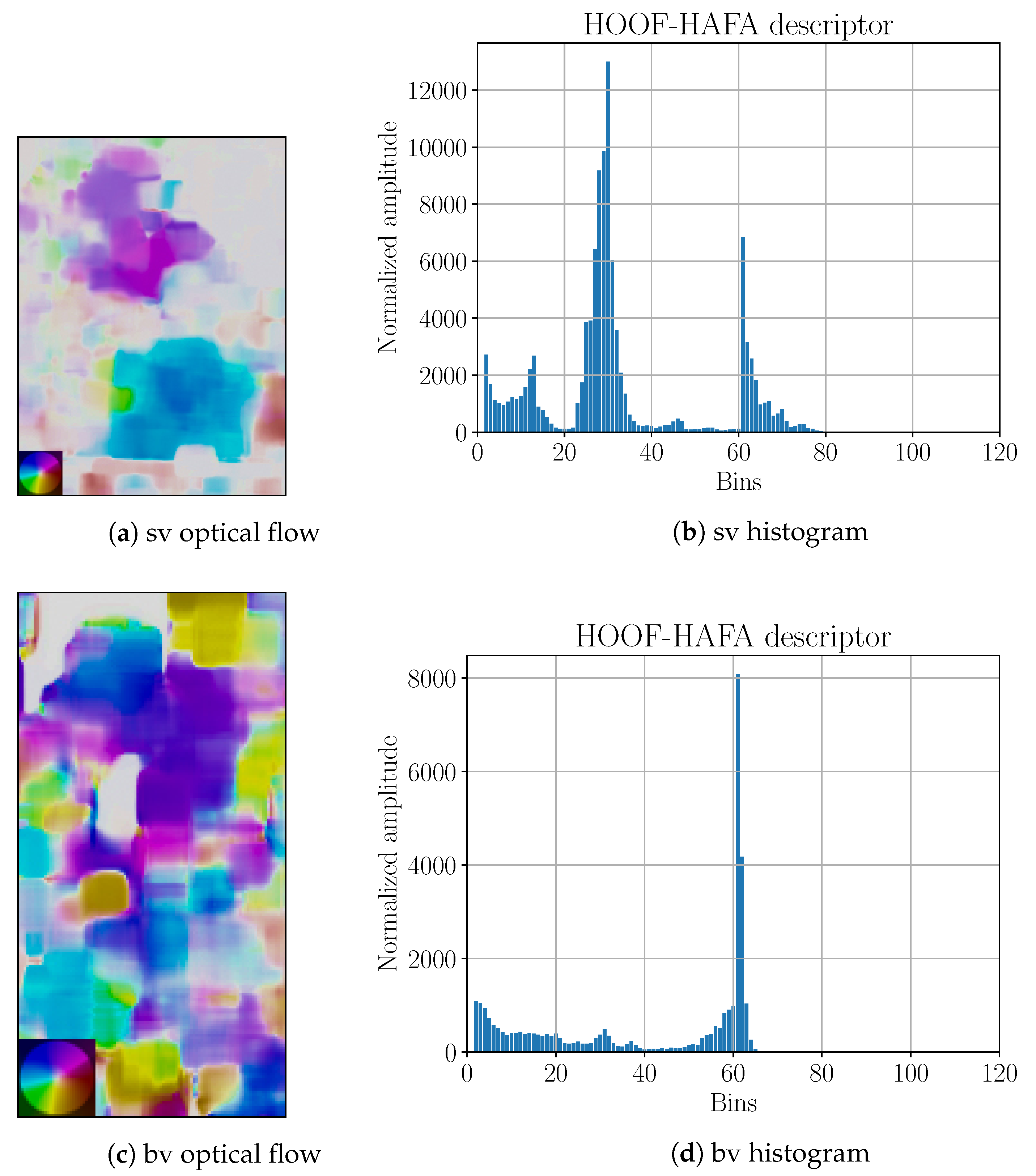
Figure 18.
Side-view (“sv”) and back-view (“bv”) optical flows with corresponding HOOF–HAFA histograms. Optical flows correspond to 24th frame in
Figure 16. Color coding legends on the lower left corners are based on [
41]. Maximal amplitude for “sv” is 28 ppf and for “bv” is 5 ppf.
Figure 18.
Side-view (“sv”) and back-view (“bv”) optical flows with corresponding HOOF–HAFA histograms. Optical flows correspond to 24th frame in
Figure 16. Color coding legends on the lower left corners are based on [
41]. Maximal amplitude for “sv” is 28 ppf and for “bv” is 5 ppf.
Figure 19.
P2SF prediction scheme. It is used for Phase 2 testing using the scene flow.
Figure 19.
P2SF prediction scheme. It is used for Phase 2 testing using the scene flow.
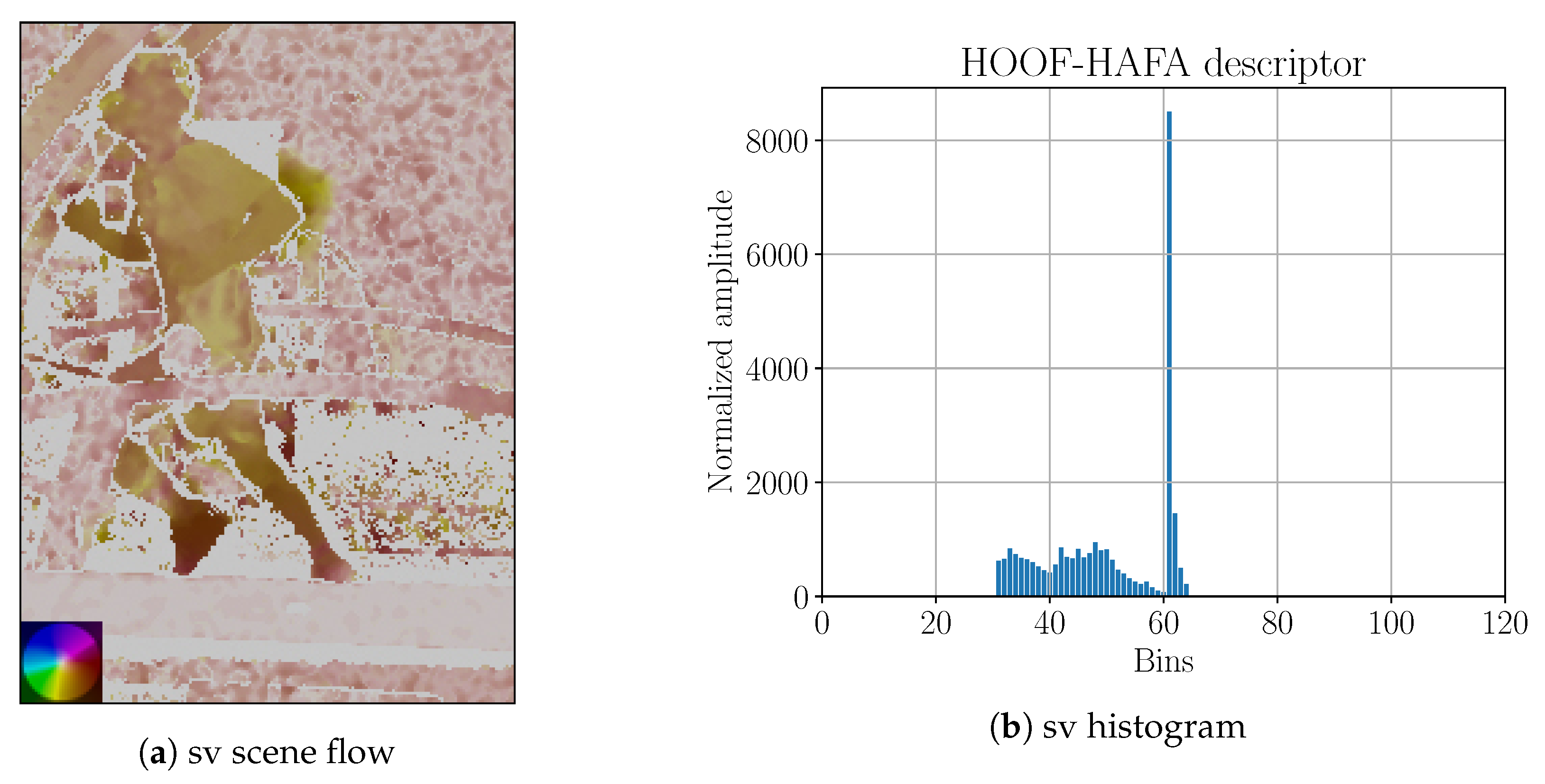
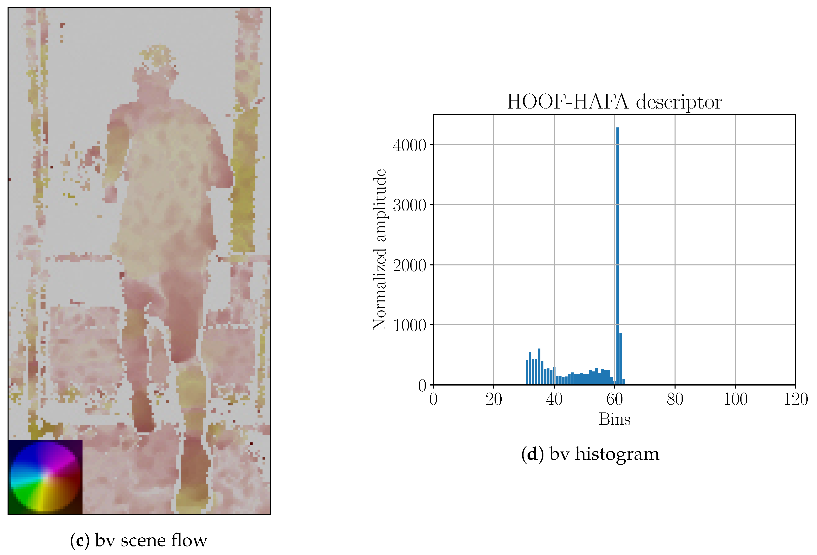
Figure 20.
Side-view (“sv”) and back-view (“bv”) projections of scene flow onto image plane with corresponding HOOF–HAFA histograms. Scene flows correspond to the frame that is shown in
Figure 16. Color coding legends on the lower left corners are based on [
41]. Maximum amplitude of projected image of the scene flow: (
a) 6 ppf; and (
c) 15 ppf.
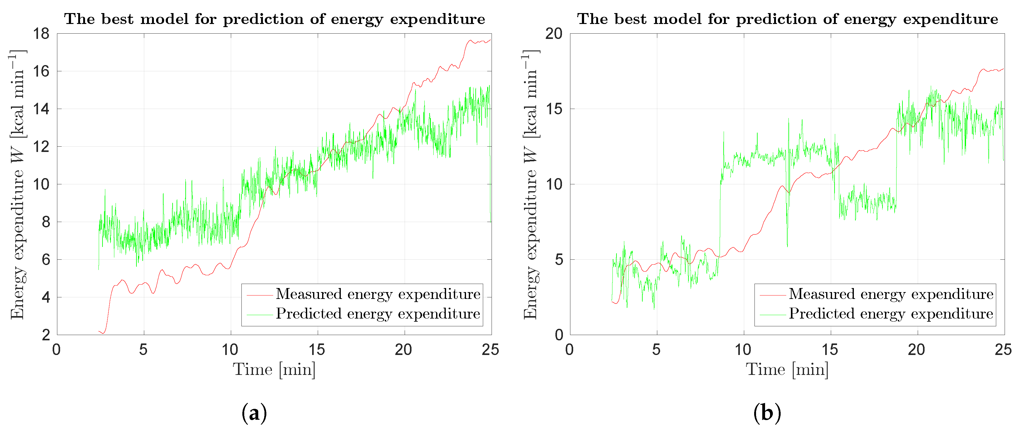
Figure 21.
Response of SUBJ8 models for Protocol 3 of Phase 2 laboratory results: (a) best results using optical flow.; and (b) best results using scene flow. Red curve represents measured data, green curve prediction.
Figure 21.
Response of SUBJ8 models for Protocol 3 of Phase 2 laboratory results: (a) best results using optical flow.; and (b) best results using scene flow. Red curve represents measured data, green curve prediction.
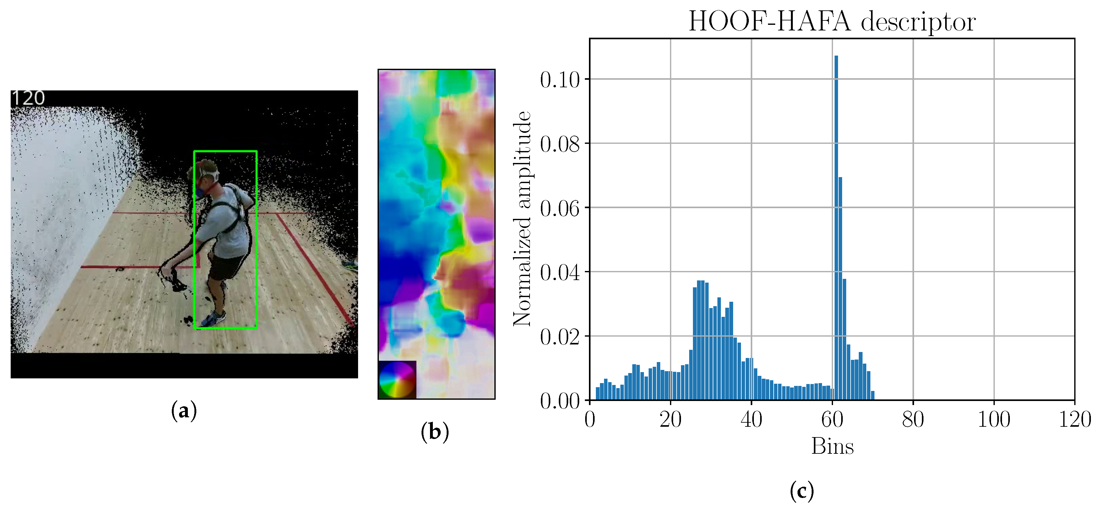
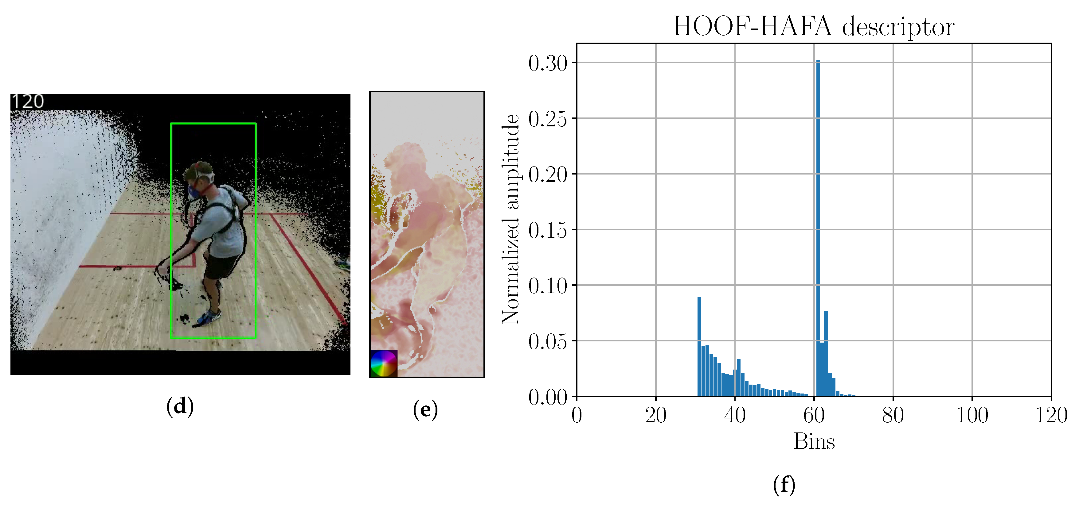
Figure 22.
Tracking results, flow field and HOOF–HAFA histogram for P2OF approach are shown in (
a–
c), respectively. Panels (
d–
f) represent results for P2SF. Color coding legend on the lower left in (
b,
e) are based on [
41]. Maximal amplitude of optical flow image is 10 ppf. Maximal amplitude of scene flow is
m s
−1.
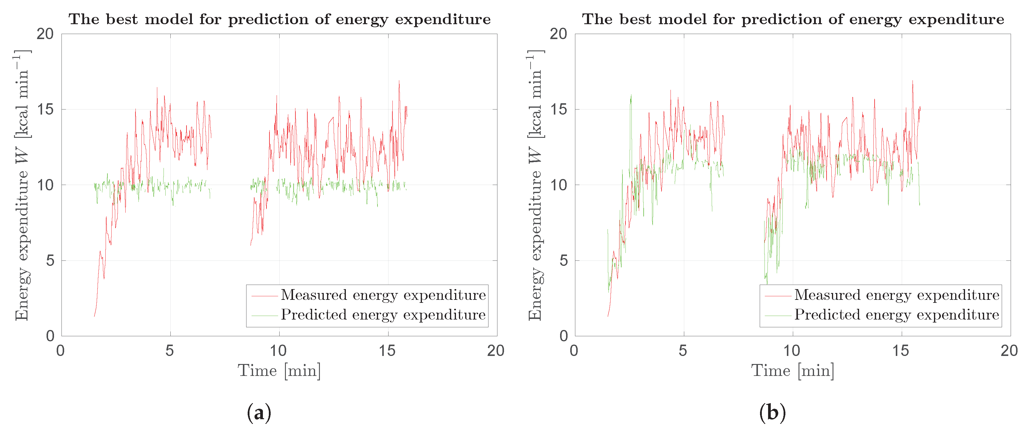
Figure 23.
Response of SUBJ9 models for Protocol 3 of Phase 2 field results: (a) best results using optical flow; and (b) best results using scene flow. Red curve represents measured data, green curve prediction.
Figure 23.
Response of SUBJ9 models for Protocol 3 of Phase 2 field results: (a) best results using optical flow; and (b) best results using scene flow. Red curve represents measured data, green curve prediction.
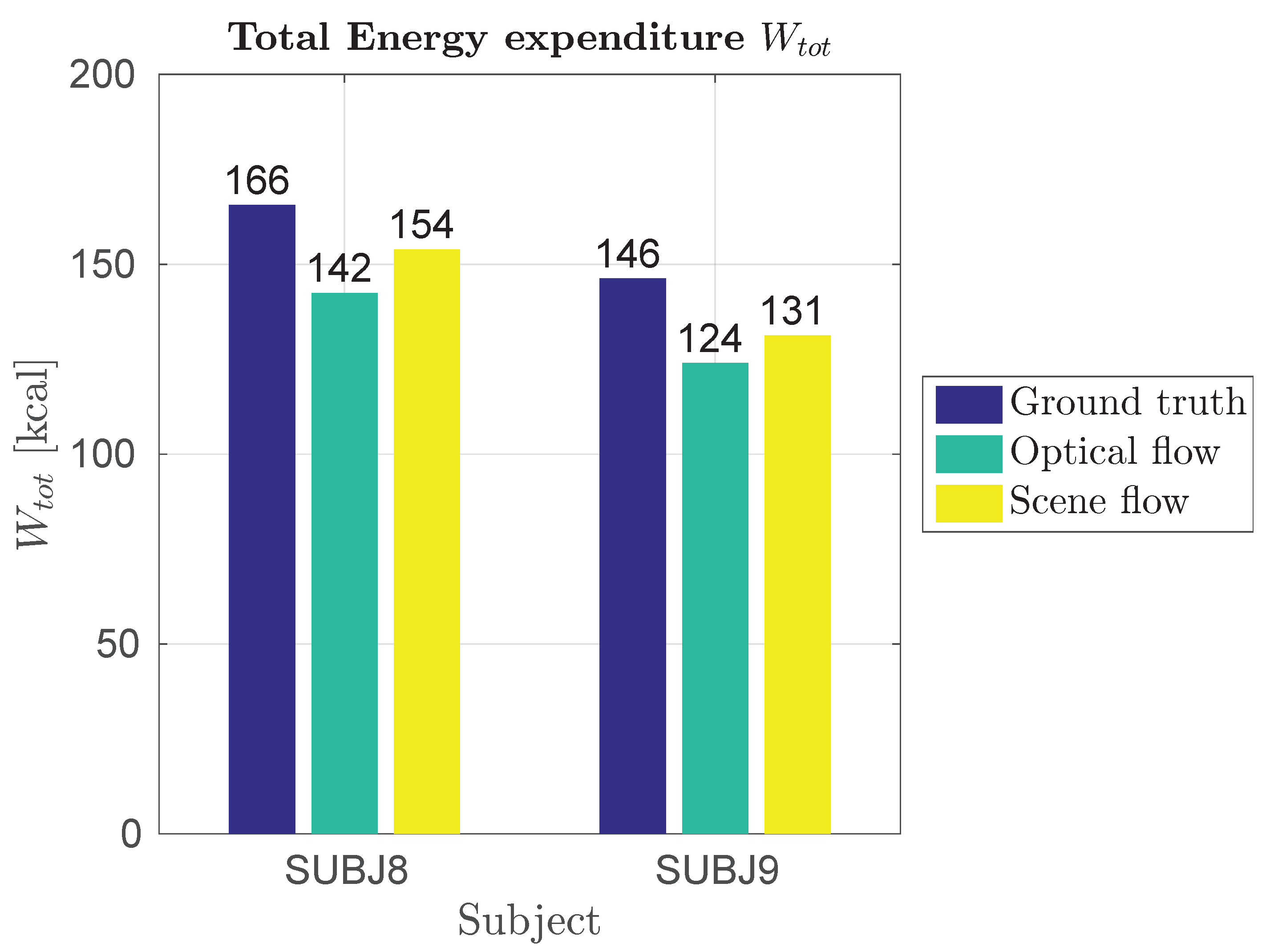
Figure 24.
Total energy expenditure for Protocol 3 of Phase 2 field results.
Figure 24.
Total energy expenditure for Protocol 3 of Phase 2 field results.
Table 1.
Anthropometric and physiological data for Subjects 0, 11 and 12.
Table 1.
Anthropometric and physiological data for Subjects 0, 11 and 12.
| Subject | SUBJ0 | SUBJ11 | SUBJ12 |
|---|
| sex | m | m | m |
| age (years) | 26 | 45 | 17 |
| height (cm) | 177 | 176 | 178 |
| weight (kg) | 79.1 | 68 | 66 |
| (mL min) | 3705 | / | / |
| (bpm) | 194 | 179 | 203 |
| (bpm) | / | 45 | 50 |
| experiments | P1L | P1C | P1C |
Table 2.
Anthropometric and physiological data for Subjects 1, 2, 4, 7, 8, 9 and 10.
Table 2.
Anthropometric and physiological data for Subjects 1, 2, 4, 7, 8, 9 and 10.
| Subject | SUBJ1 | SUBJ2 | SUBJ4 | SUBJ7 | SUBJ8 | SUBJ9 | SUBJ10 |
|---|
| sex | m | m | m | m | m | m | m |
| age (years) | 20 | 14 | 15 | 15 | 19 | 15 | 16 |
| height (cm) | 174 | 151.7 | 186 | 174.4 | 185 | 175 | 181.5 |
| weight (kg) | 66.8 | 35.2 | 61.9 | 62.9 | 72.8 | 62 | 53.9 |
| (mL min) | 3418 | 1908 | 3608 | 3486 | 3413 | 3513 | 2662 |
| (bpm) | 200 | 206 | 205 | 205 | 201 | 205 | 204 |
| (bpm) | / | / | / | / | / | / | / |
| experiments | P2L, P2C | P2L, P2C | P2L | P2L, P2C | P2L, P2C | P2L, P2C | P2C |
Table 3.
Overview of the experiments performed. Experiment names have been constructed as P1/P2 for Phase1/Phase2, L for laboratory, and C for court.
Table 3.
Overview of the experiments performed. Experiment names have been constructed as P1/P2 for Phase1/Phase2, L for laboratory, and C for court.
| Experiment | P1L | P1C | P2L | P2C |
|---|
| environment | physiology laboratory | squash court | physiology laboratory | squash court |
| equipment | Cosmed K4B2 | Polar Vintage NV | Cosmed K4B2 | Cosmed K4B2 |
| parameter | eem(t), hr(t) | hr(t) | eem(t) | eem(t) |
| camera modality | RGB, NIR | RGB | RGB, RGBD | RGB, RGBD |
| camera position | lateral, posterior | posterior | lateral, posterior | posterior |
| camera type | Axis 207W IP camera | RaspiCam | Microsoft Kinect V2 | Microsoft Kinect V2 |
| motion data | optical flow | optical flow | optical, scene flow | optical, scene flow |
| tracker | / | KCF | KCF, DS-KCF | KCF, DS-KCF |
| descriptor | HOOF | HOOF–HAFA | HOOF–HAFA | HOOF–HAFA |
| model | -SVR + RBF | -SVR + RBF | -RBF | -RBF |
| filter | Kalman | Gaussian | Gaussian | Gaussian |
Table 4.
Validation measures for observability test. These are average values of sv and bv models. Pearson correlations were averaged using Fisher z transform. Best results shown in bold.
Table 4.
Validation measures for observability test. These are average values of sv and bv models. Pearson correlations were averaged using Fisher z transform. Best results shown in bold.
| Model | CORR | RAE | RRSE | nSV |
|---|
| eem | 0.86 | 0.46 | 0.53 | 0.54 |
| hr | 0.89 | 0.78 | 0.78 | 0.768 |
Table 5.
Validation measures for viewpoint modality tests. Best results are shown in bold.
Table 5.
Validation measures for viewpoint modality tests. Best results are shown in bold.
| Model | CORR | RAE | RRSE | nSV |
|---|
| eem-bv(bv) | 0.83 | 0.48 | 0.58 | 0.60 |
| eem-bv(sv) | −0.83 | 1.37 | 1.54 | 0.60 |
| eem-sv(bv) | −0.48 | 1.22 | 1.28 | 0.59 |
| eem-sv(sv) | 0.86 | 0.46 | 0.52 | 0.59 |
| eem-mixed(bv) | 0.84 | 0.57 | 0.63 | 0.62 |
| eem-mixed(sv) | 0.85 | 0.46 | 0.54 | 0.62 |
| hr-bv(bv) | 0.87 | 0.75 | 0.75 | 0.87 |
| hr-bv(sv) | −0.86 | 2.13 | 2.15 | 0.87 |
| hr-sv(bv) | 0.33 | 1.08 | 1.22 | 0.85 |
| hr-sv(sv) | 0.90 | 0.71 | 0.72 | 0.85 |
| hr-mixed(bv) | 0.88 | 0.60 | 0.62 | 0.74 |
| hr-mixed(sv) | 0.89 | 0.67 | 0.68 | 0.74 |
Table 6.
Validation measures for image type (BGR or NIR) modality tests. Best results shown in bold.
Table 6.
Validation measures for image type (BGR or NIR) modality tests. Best results shown in bold.
| Model | CORR | RAE | RRSE | nSV |
|---|
| eem-bv(bv) | 0.83 | 0.48 | 0.58 | 0.60 |
| eem-nir(nir) | 0.86 | 0.47 | 0.53 | 0.58 |
| hr-bv(bv) | 0.87 | 0.75 | 0.75 | 0.87 |
| hr-nir(nir) | 0.90 | 0.67 | 0.69 | 0.73 |
Table 7.
Validation measures for field testing. HOOF and HOOF–HAFA descriptors are used. Models are overfitted.
Table 7.
Validation measures for field testing. HOOF and HOOF–HAFA descriptors are used. Models are overfitted.
| Model | CORR | RAE | RRSE | nSV |
|---|
| hr-bv-hoof(bv) | 0.00 | 1.45 | 1.46 | 0.00 |
| hr-bv-hoofhafa(bv) | 0.34 | 0.97 | 0.98 | 0.98 |
Table 8.
Amplitude factors for each subject and camera viewpoint.
Table 8.
Amplitude factors for each subject and camera viewpoint.
| Viewpoint | Subject | | Viewpoint | Subject | |
|---|
| back-view | 1 | 208.557 | side-view | 1 | 236.985 |
| 2 | 179.011 | 2 | 163.957 |
| 4 | 225.568 | 4 | 196.461 |
| 7 | 195.133 | 7 | 205.760 |
| 8 | 209.991 | 8 | 190.253 |
| 9 | 182.003 | 9 | 178.16 |
Table 9.
Average validation measures for Protocol 1 of Phase 2 laboratory results. Pearson correlations were averaged using Fisher z transform. Best results shown in bold.
Table 9.
Average validation measures for Protocol 1 of Phase 2 laboratory results. Pearson correlations were averaged using Fisher z transform. Best results shown in bold.
| Model | CORR | RAE | RRSE | nSV |
|---|
| eem-bv-of(bv) | 0.97 | 0.35 | 0.38 | 0.33 |
| eem-sv-of(sv) | 0.98 | 0.20 | 0.23 | 0.27 |
| eem-bv-sf(bv) | 0.97 | 0.26 | 0.30 | 0.33 |
| eem-sv-sf(sv) | 0.99 | 0.12 | 0.15 | 0.26 |
Table 10.
Average validation measures for Protocol 2 of Phase 2 laboratory results. Pearson correlations were averaged using Fisher z transform. Best results shown in bold.
Table 10.
Average validation measures for Protocol 2 of Phase 2 laboratory results. Pearson correlations were averaged using Fisher z transform. Best results shown in bold.
| Model | CORR | RAE | RRSE | nSV |
|---|
| eem-bv-of(bv) | −0.51 | 4.71 | 4.24 | 0.30 |
| eem-sv-of(sv) | −0.69 | 4.26 | 3.93 | 0.22 |
| eem-bv-sf(bv) | −0.51 | 4.89 | 4.59 | 0.35 |
| eem-sv-sf(sv) | −0.29 | 4.23 | 3.93 | 0.26 |
Table 11.
Validation measures for Protocol 3 of Phase 2 laboratory results. Best results shown in bold.
Table 11.
Validation measures for Protocol 3 of Phase 2 laboratory results. Best results shown in bold.
| Model | CORR | RAE | RRSE | nSV |
|---|
| eem-bv-of-subj8(bv) | 0.95 | 0.50 | 0.52 | 0.30 |
| eem-bv-of-subj9(bv) | 0.95 | 0.55 | 0.57 | 0.30 |
| eem-sv-of-subj8(sv) | 0.96 | 0.34 | 0.39 | 0.18 |
| eem-sv-of-subj9(sv) | 0.93 | 0.59 | 0.69 | 0.18 |
| eem-bv-sf-subj8(bv) | 0.79 | 0.58 | 0.63 | 0.33 |
| eem-bv-sf-subj9(bv) | 0.68 | 1.00 | 1.12 | 0.33 |
| eem-sv-sf-subj8(sv) | 0.14 | 1.16 | 1.29 | 0.22 |
| eem-sv-sf-subj9(sv) | 0.78 | 0.74 | 0.82 | 0.22 |
Table 12.
Average validation measures for Protocol 1 of Phase 2 field results. Pearson correlations were averaged using Fisher z transform. Best results shown in bold.
Table 12.
Average validation measures for Protocol 1 of Phase 2 field results. Pearson correlations were averaged using Fisher z transform. Best results shown in bold.
| Model | CORR | RAE | RRSE | nSV |
|---|
| eem-bv-of(bv) | 0.54 | 0.94 | 0.91 | 0.48 |
| eem-bv-sf(bv) | 0.76 | 0.66 | 0.65 | 0.41 |
Table 13.
Average validation measures for Protocol 2 of Phase 2 field results. Pearson correlations were averaged using Fisher z transform. Best results shown in bold.
Table 13.
Average validation measures for Protocol 2 of Phase 2 field results. Pearson correlations were averaged using Fisher z transform. Best results shown in bold.
| Model | CORR | RAE | RRSE | nSV |
|---|
| eem-bv-of(bv) | −0.05 | 1.41 | 1.34 | 0.41 |
| eem-bv-sf(bv) | 0.00 | 1.77 | 1.67 | 0.41 |
Table 14.
Validation measures for Protocol 3 of Phase 2 field results. Best results shown in bold.
Table 14.
Validation measures for Protocol 3 of Phase 2 field results. Best results shown in bold.
| Model | CORR | RAE | RRSE | nSV |
|---|
| eem-bv-of-subj8(bv) | 0.02 | 1.27 | 1.17 | 0.29 |
| eem-bv-of-subj9(bv) | 0.02 | 1.29 | 1.13 | 0.29 |
| eem-bv-sf-subj8(bv) | 0.41 | 1.02 | 0.99 | 0.41 |
| eem-bv-sf-subj9(bv) | 0.72 | 0.89 | 0.83 | 0.41 |


