Forecasting of Cereal Yields in a Semi-arid Area Using the Simple Algorithm for Yield Estimation (SAFY) Agro-Meteorological Model Combined with Optical SPOT/HRV Images


Abstract
:1. Introduction
2. Experimental Database
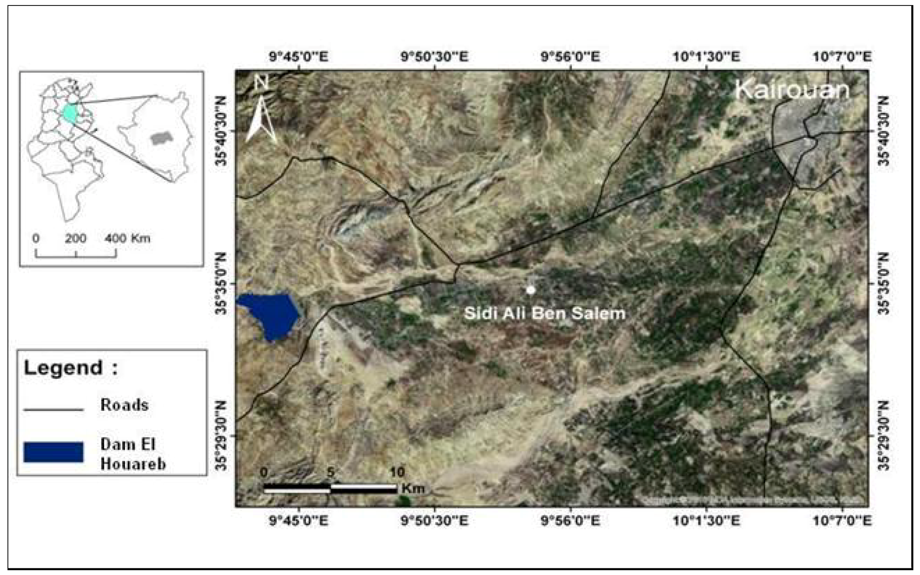
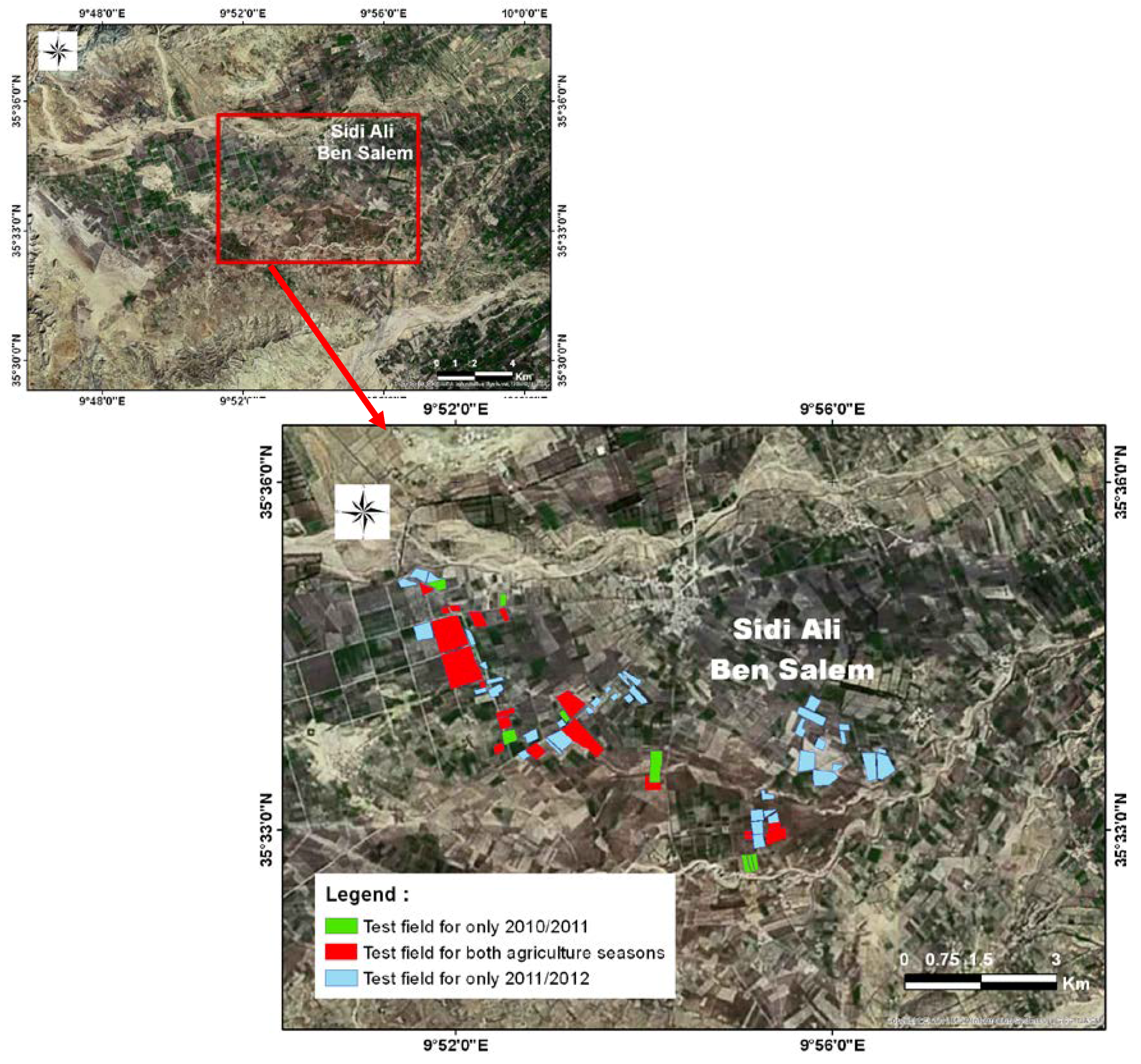
2.1. Study Area
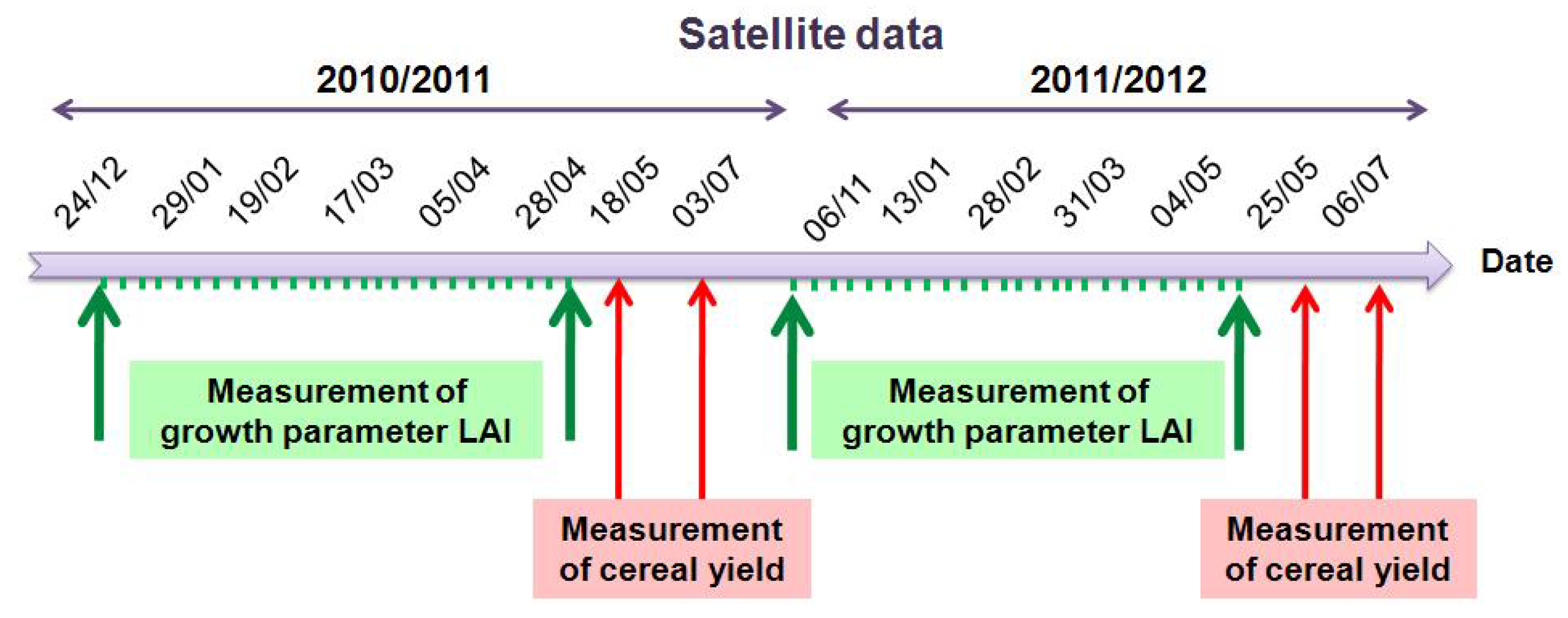
2.2. Satellite Data
2.3. Ground Measurements
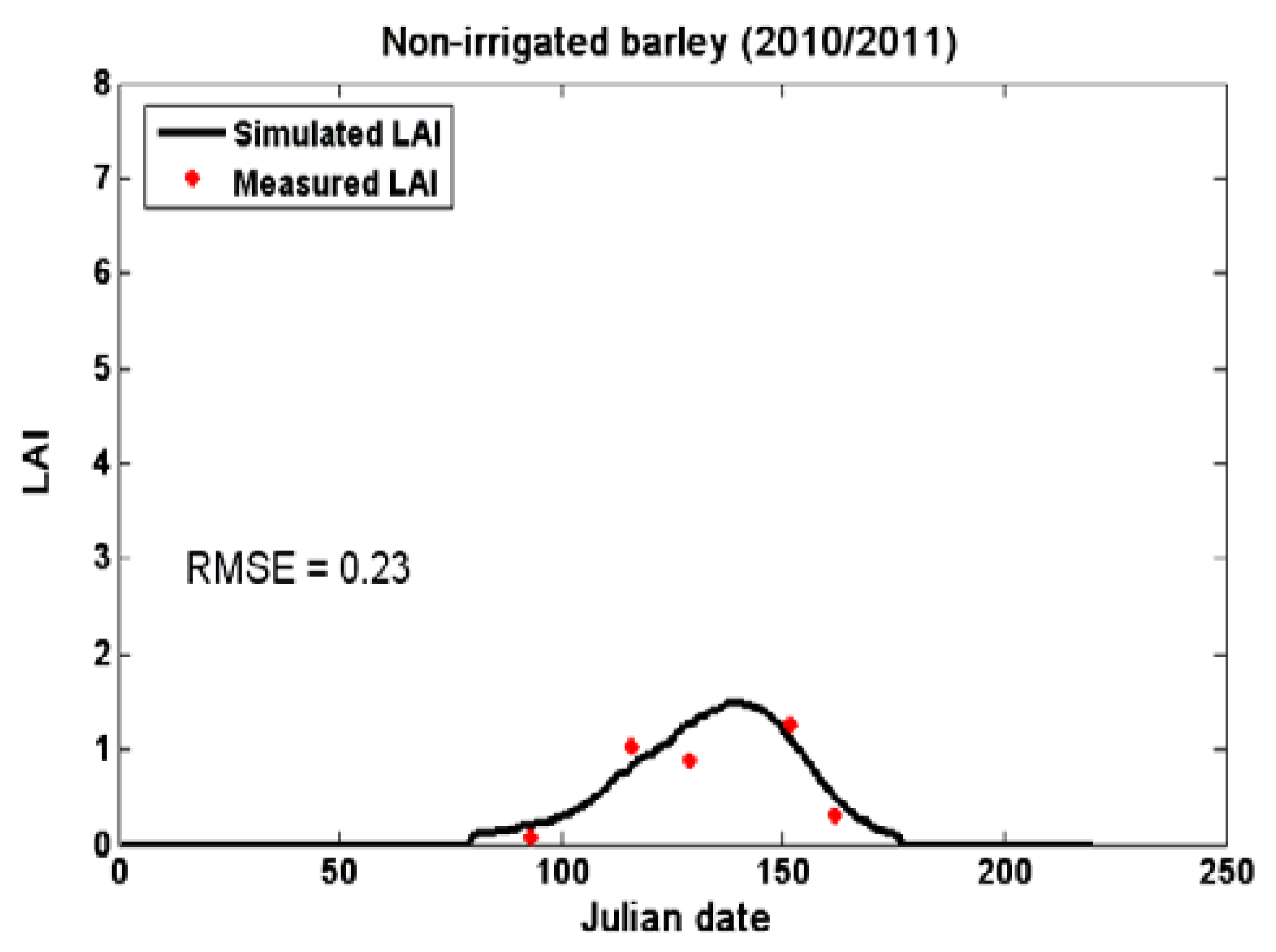
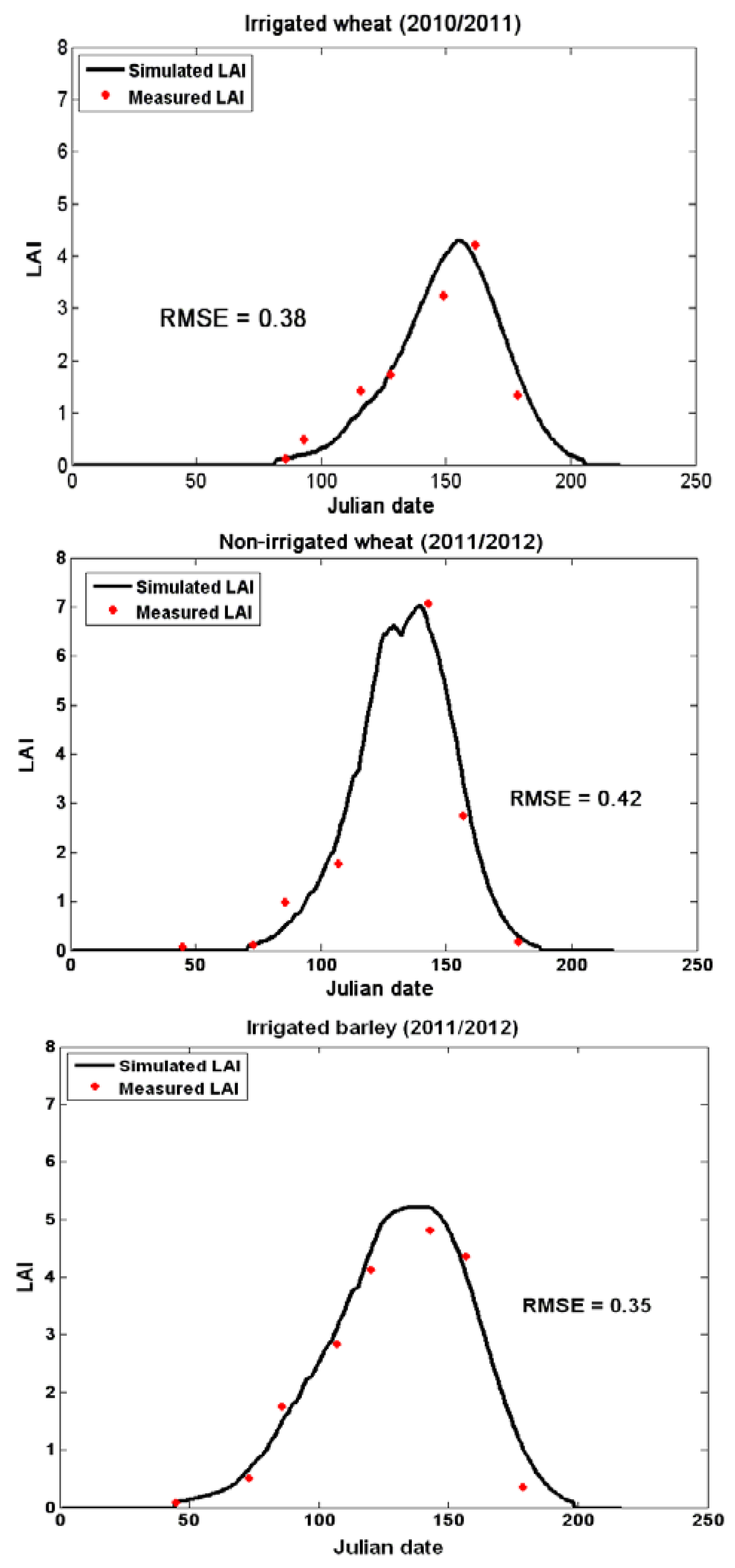
2.3.1. Leaf Area Index
2.3.2. Cereal Yield
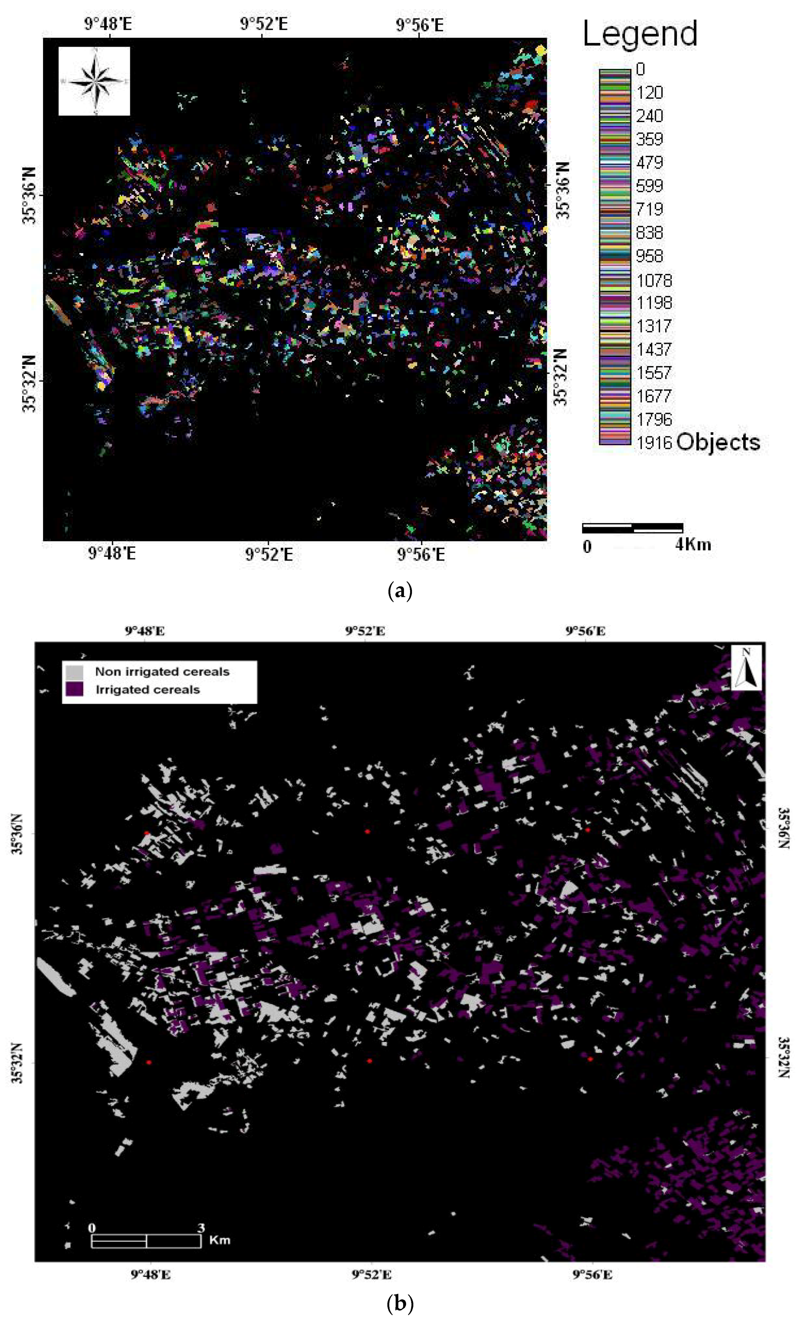
2.4. Classification of Satellite Images over the Kairouan Plain
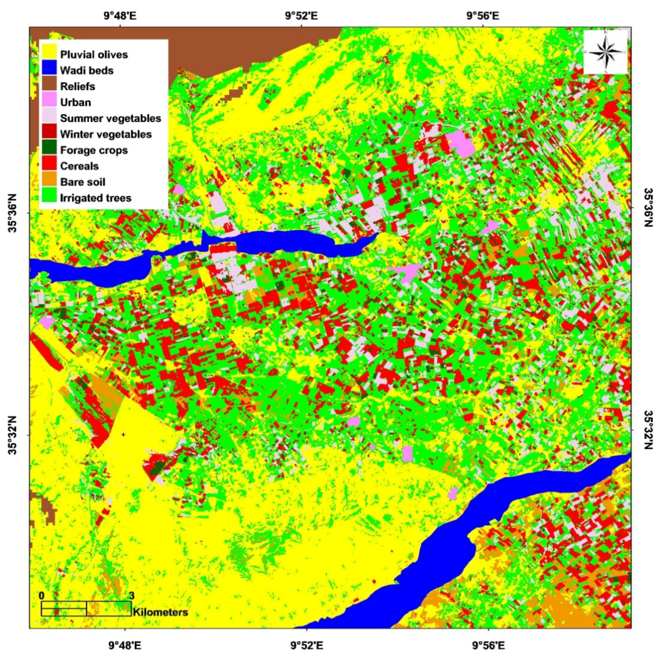
2.4.1. Land Use Map
2.4.2. Classification of Irrigated and Non-Irrigated Cereals
3. Methodology for the Estimation of Cereal Yields Using the SAFY Growth Model
3.1. SAFY Model Description
3.2. Application of SAFY to Cereal Cycle Retrieval
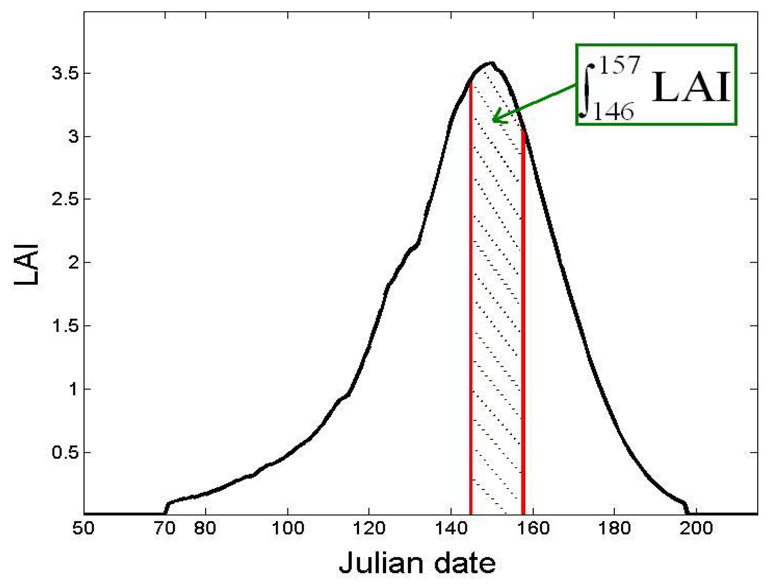
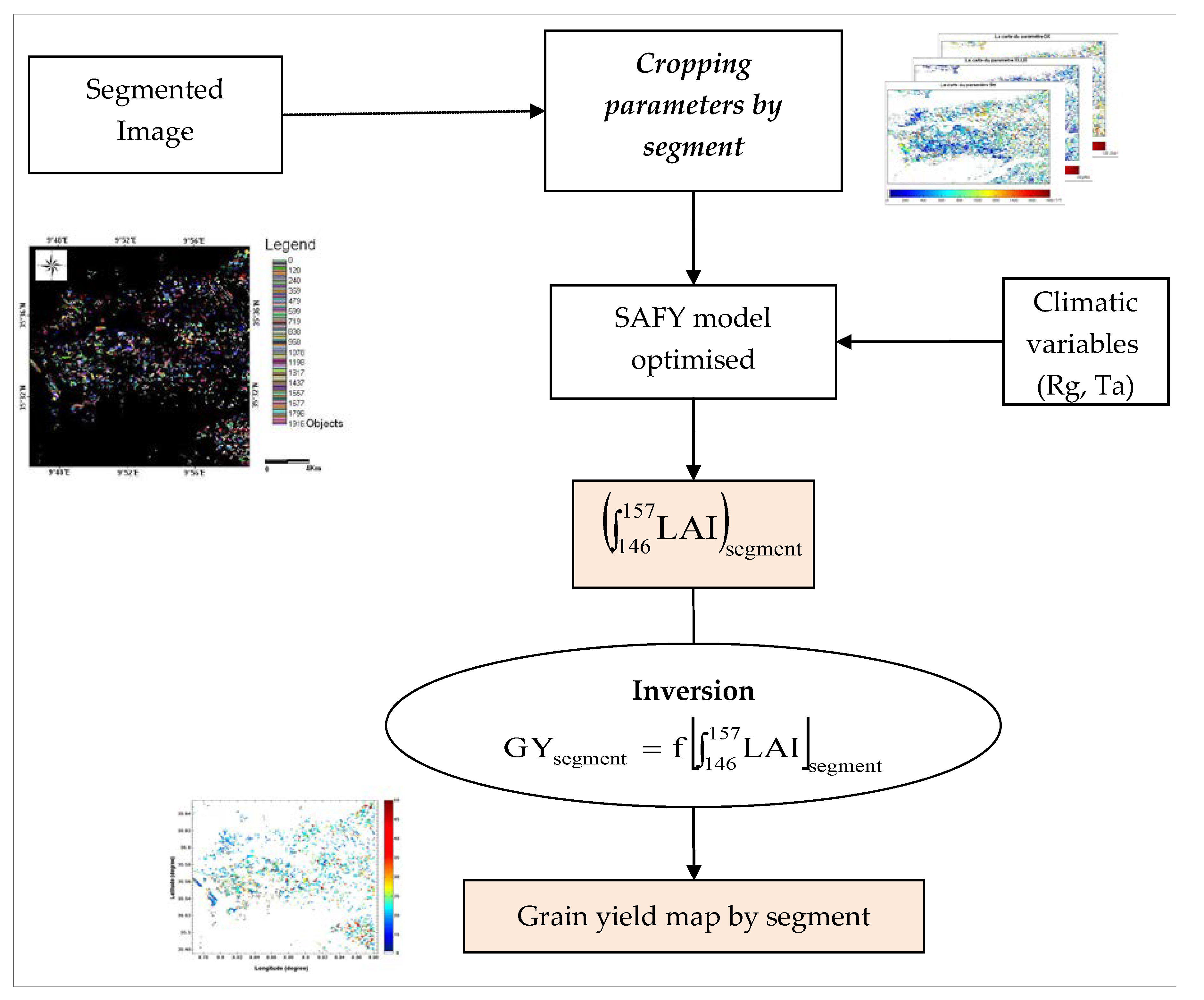
3.3. Proposed Approach
4. Results and Discussions
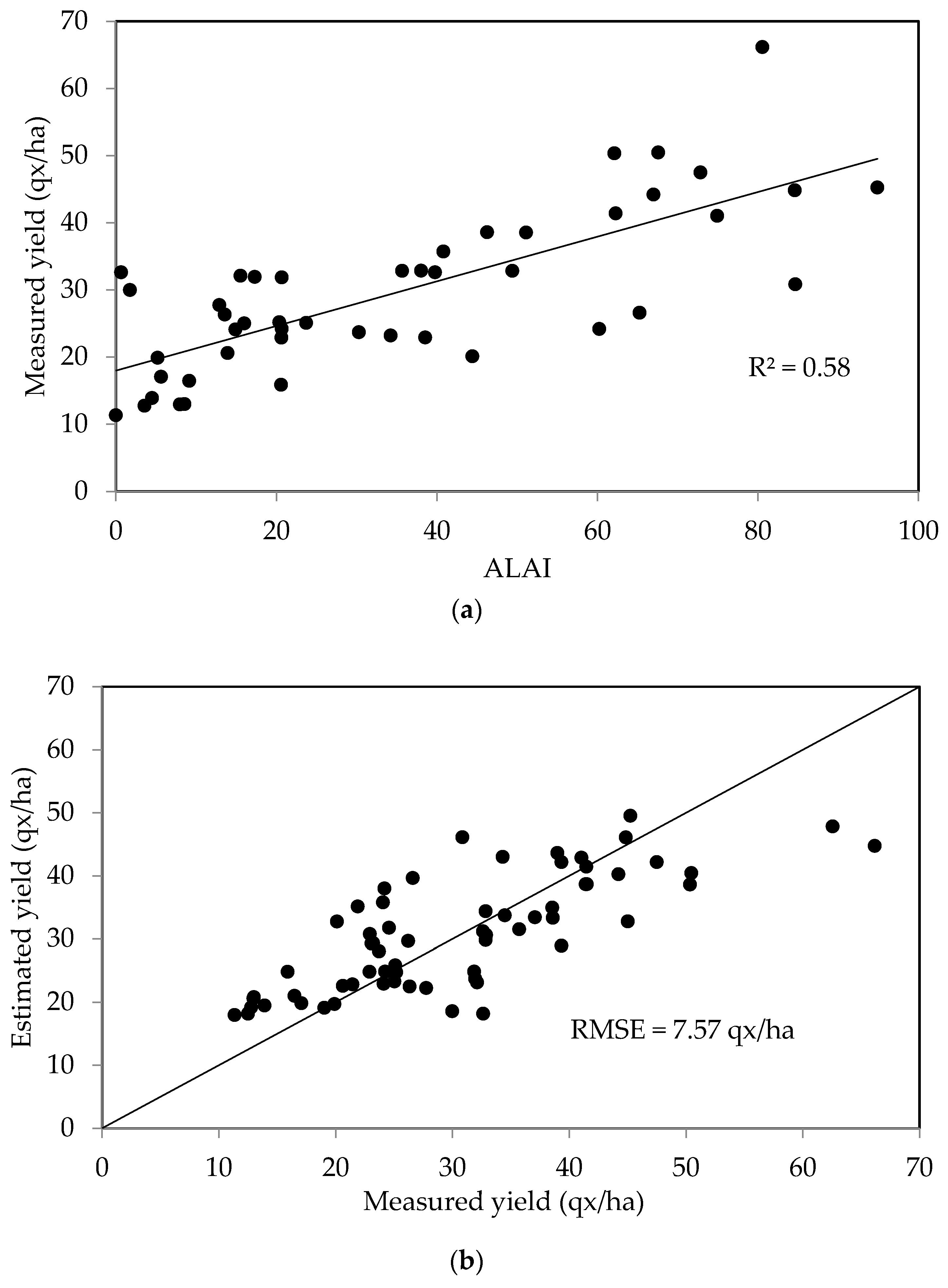
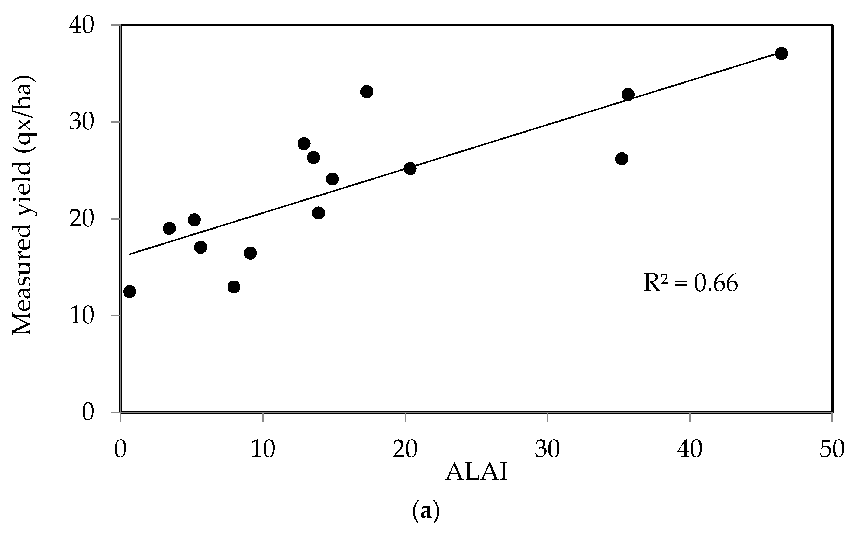
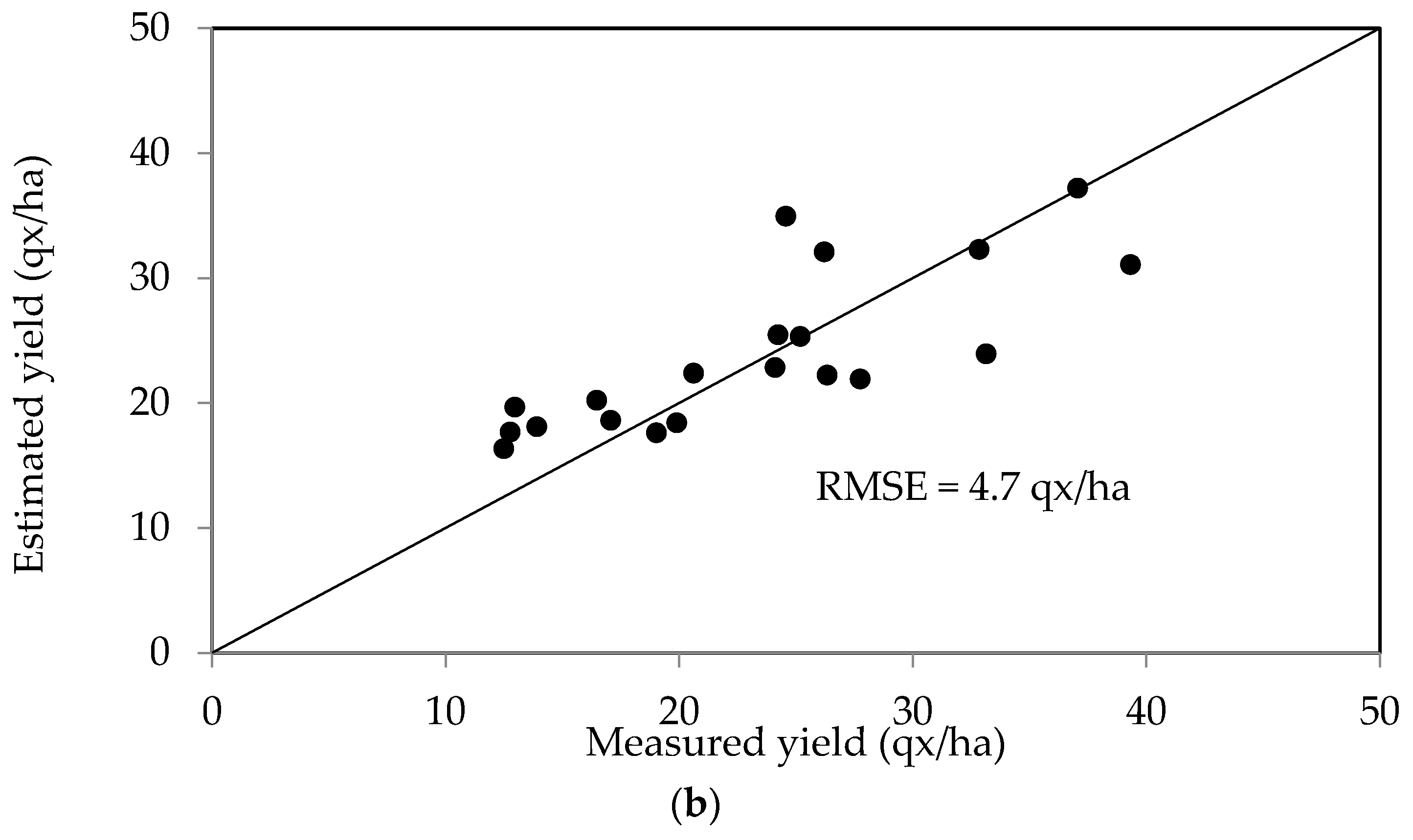
4.1. Estimating the Yields of All Cereals
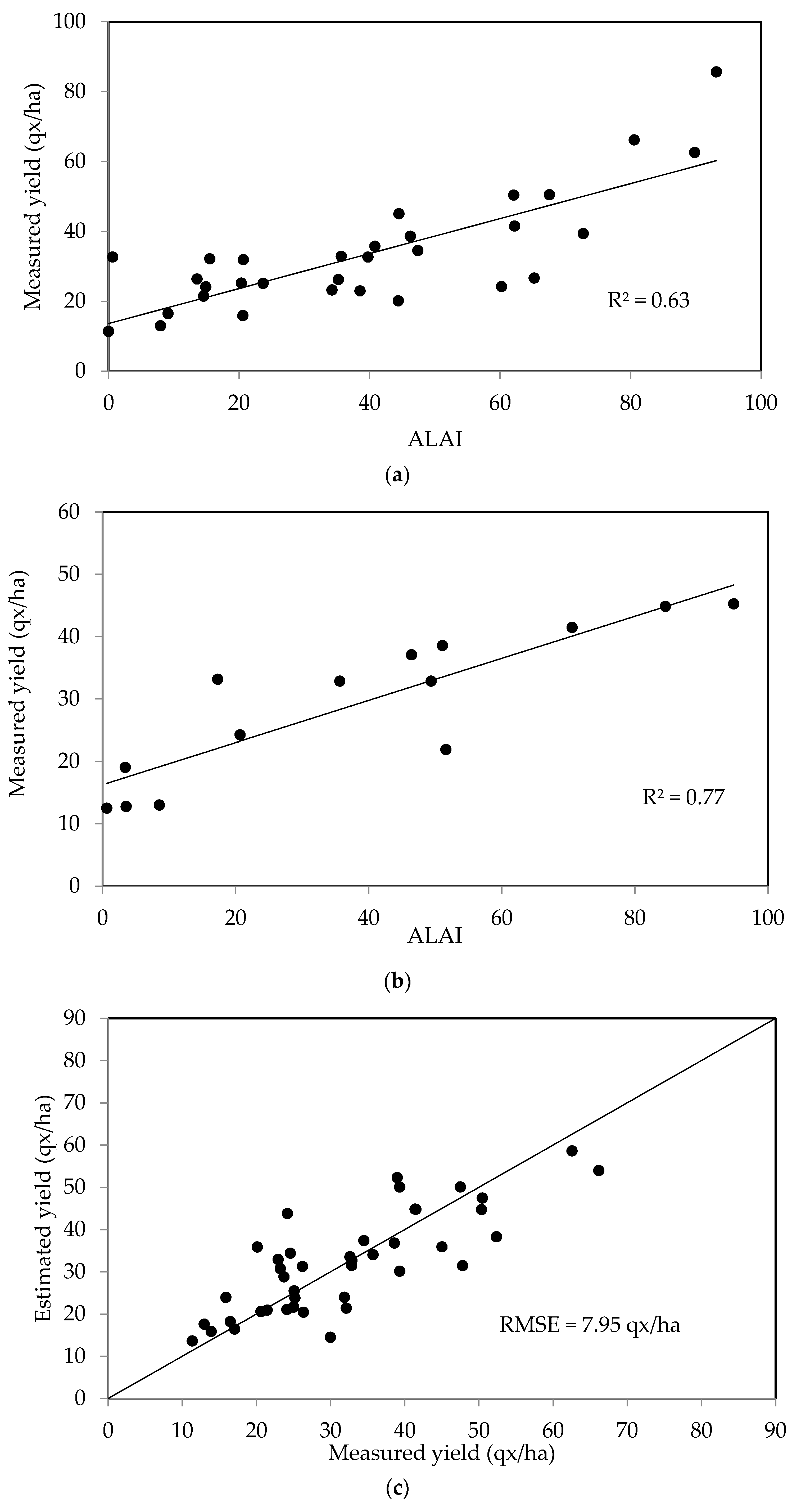
4.2. Wheat and Barley Yield Estimations
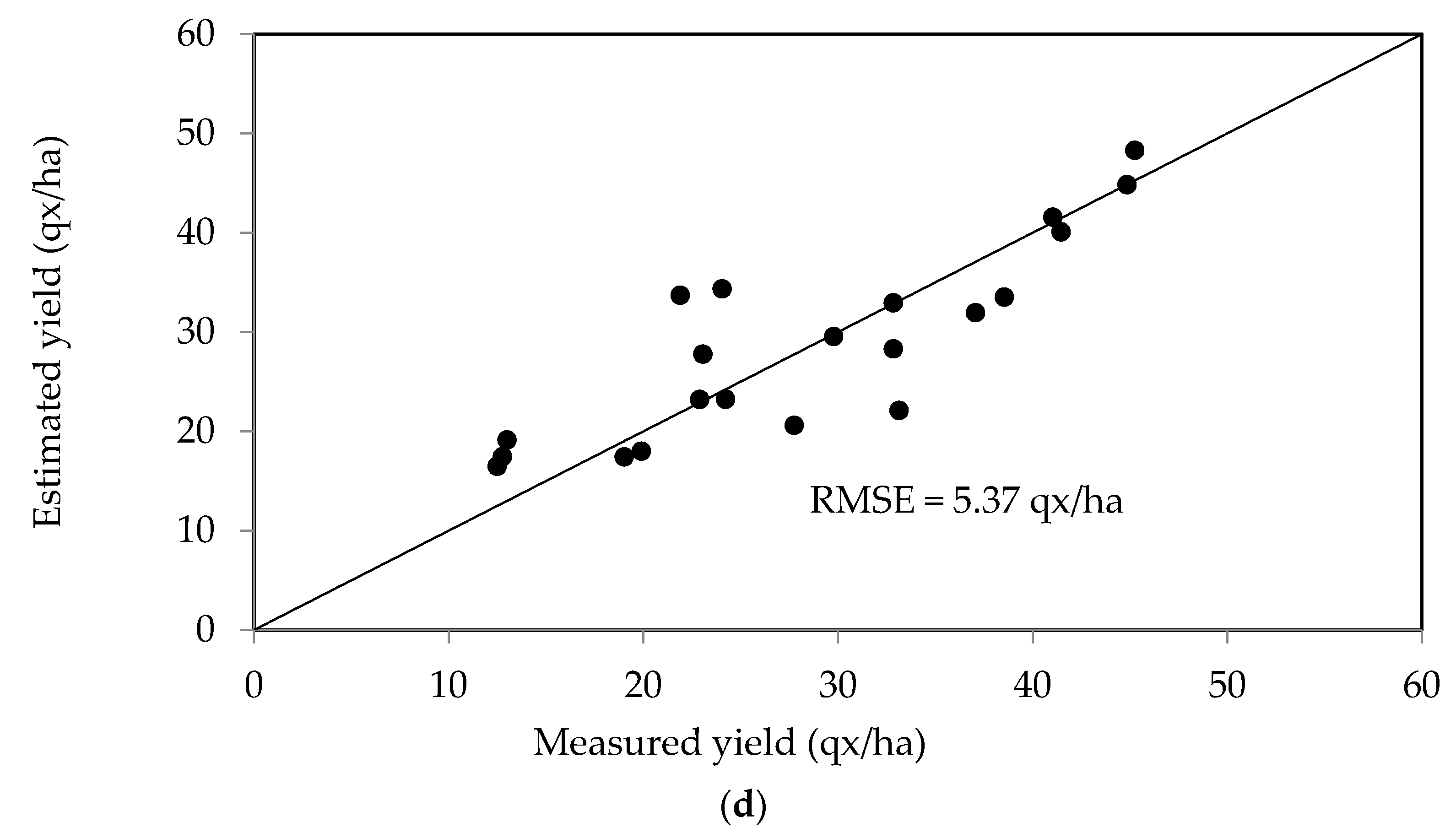
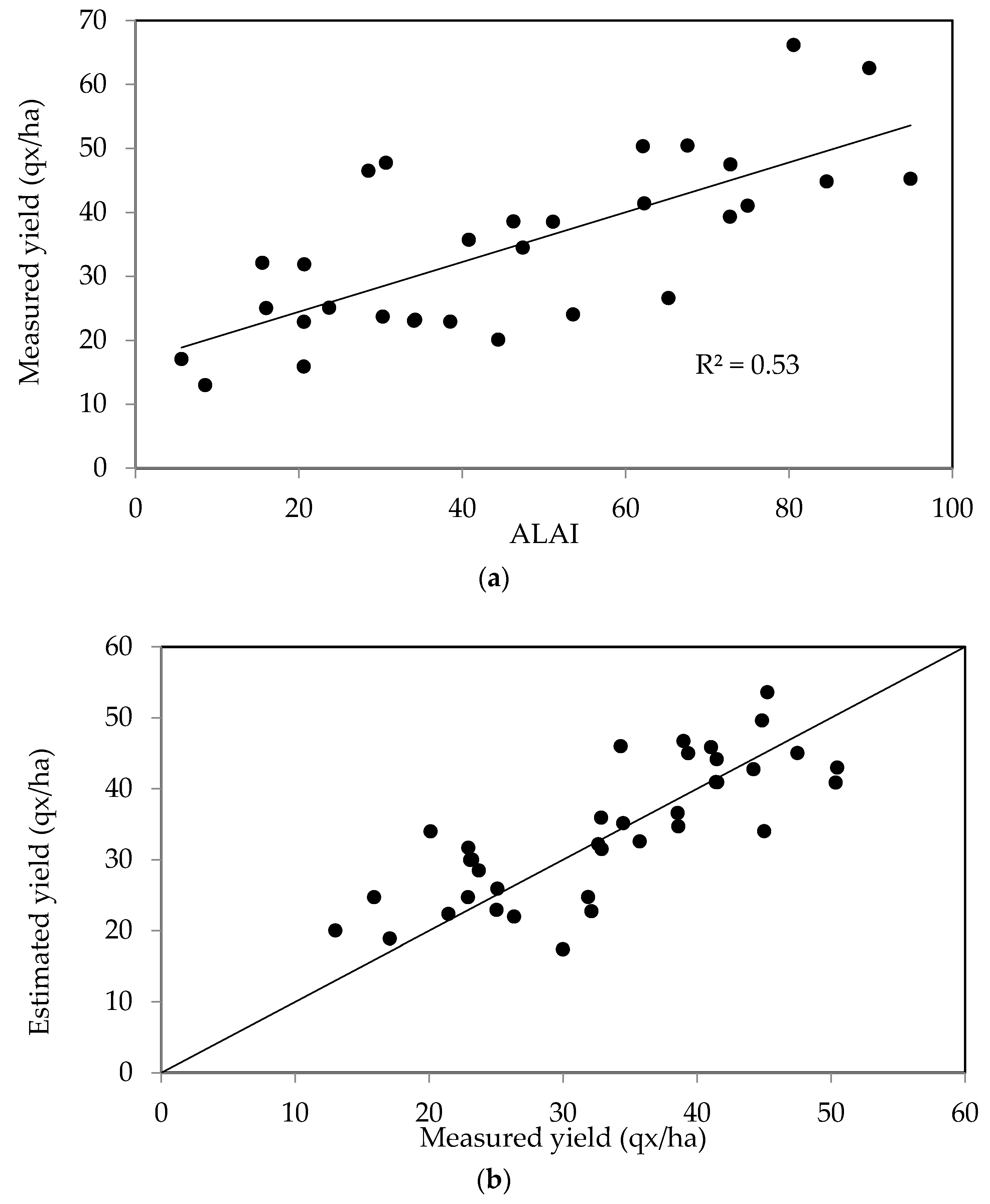
4.3. Yield Estimations for Irrigated and Non-Irrigated Areas
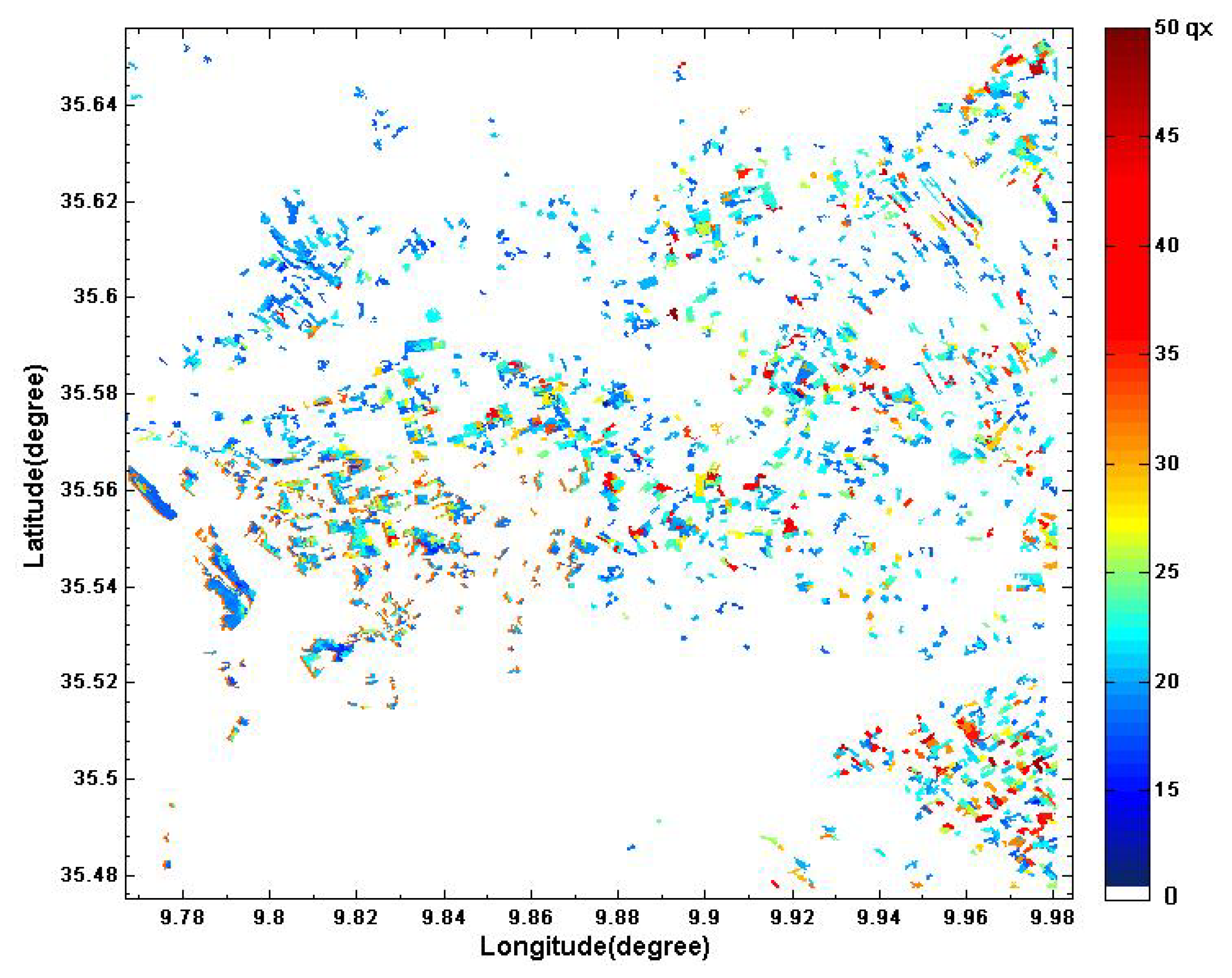
4.4. Spatialisation of Grain Yield
5. Conclusions
Author Contributions
Funding
Conflicts of Interest
References
- Palmieri, L.; Amantonico, B. Rapport Etude de Faisabilité: Etude D’identification pour la Mise en Œuvre de L’observation Agro-Alimentaire Italo-Tunisien. Programme “Instrument Européen de Voisinage et de Partenariat de Coopération Transfrontalière (IEVP CT) Italie-Tunisie 2007–2013”. 2013, p. 23. Available online: servagri.eu/index.php/fr/documentation/etude-de-faisabilite?...15:etude...faisabilite (accessed on 20 April 2016).
- Justice, C.O.; Becker-Reshef, I. Report from the Workshop on Developing a Strategy for Global Agricultural Monitoring in the Framework of Group on Earth Observations (GEO). 2007, pp. 1–67. Available online: http://www.fao.org/gtos/igol/docs/meeting-reports/07-geo-ag0703-workshop-report-nov07.pdf (accessed on 11 June 2015).
- Fratanellli, G.; Paloscia, S.; Zribi, M.; Chahbi, A. Sensitivity analysis of X-band SAR to wheat and barley biomass in the Merguellil Basin. Remote Sens. Lett. 2013, 4, 1107–1116. [Google Scholar]
- Fieuzal, R.; Duchemin, B.; Jarlan, L.; Zribi, M.; Baup, F.; Merlin, O.; Dedieu, G.; Garatuza-Payan, J.; Watt, C.; Chehbouni, A. Combined use of optical and radar satellite data for the monitoring of irrigation and soil moisture of wheat crops. Hydrol. Earth Syst. Sci. 2011, 15, 1117–1129. [Google Scholar] [CrossRef] [Green Version]
- Barnett, T.L.; Thompson, D.R. The use of large-area spectral data in wheat yield estimation. Remote Sens. Environ. 1982, 12, 509–518. [Google Scholar] [CrossRef]
- Moriondo, M.; Maselli, F.; Bindi, M. A simple model of regional wheat yield based on NDVI data. Eur. J. Agron. 2007, 26, 266–274. [Google Scholar] [CrossRef]
- Baghdadi, N.; Zribi, M. Land Surface Remote Sensing in Agriculture and Forest; ISTE Press: London, UK; Elsevier: Oxford, UK, 2016; ISBN 9781785481031. [Google Scholar]
- Laguette, S.; Vidal, A.; Vossen, P. Télédétection et estimation des rendements en blé en Europe. Ingénieries–EAT 1997, 12, 19–33. [Google Scholar]
- Huete, A.; Didan, K.; Miura, T.; Rodriguez, E.P.; Gao, X.; Ferreira, L.G. Overview of the radiometric and biophysical performance of the MODIS vegetation indices. Remote Sens. Environ. 2002, 83, 195–213. [Google Scholar] [CrossRef]
- Johnson, D.M. A comprehensive assessment of the correlations between field crop yields and commonly used MODIS products. Int. J. Appl. Earth Obs. Geoinf. 2016, 52, 65–81. [Google Scholar] [CrossRef] [Green Version]
- Becker-Reshef, I.; Vermote, E.; Lindeman, M.; Justice, C. A generalized regression-based model for forecasting winter wheat yields in Kansas and Ukraine using MODIS data. Remote Sens. Environ. 2010, 114, 1312–1323. [Google Scholar] [CrossRef]
- Franch, B.; Vermote, E.F.; Becker-Reshef, I.; Claverie, M.; Huangc, J.; Zhang, J.; Justice, C.; Sobrinod, J.A. Improving the timeliness of winter wheat production forecast in the United States of America, Ukraine and China using MODIS data and NCAR Growing Degree Day information. Remote Sens. Environ. 2015, 161, 131–148. [Google Scholar] [CrossRef]
- Chahbi, A.; Zribi, M.; Lili-Chabaane, Z.; Duchemin, B.; Shabou, M.; Mougenot, B.; Boulet, G. Estimation of the dynamics and yields of cereals in a semi-arid area using remote sensing and the SAFY growth model. Int. J. Remote Sens. 2014, 35, 1004–1028. [Google Scholar] [Green Version]
- Moulin, C. Assimilation D’observations Satellitaires Courtes Longueurs D’onde dans un Modèle de Fonctionnement de Culture. Ph.D. Thesis, l’Université Paul Sabatier de Toulouse, Toulouse, France, 1995. [Google Scholar]
- Bastiaanssen, W.G.M.; Ali, S. A new crop yield forecasting model based on satellite measurements applied across the Indus Basin, Pakistan. Agric. Ecosyst. Environ. 2003, 94, 321–340. [Google Scholar] [CrossRef]
- Duchemin, B.; Maisongrande, P.; Boulet, G.; Benhadj, I. A simple algorithm for yield estimates: Evaluation for semi-arid irrigated winter wheat monitored with green leaf area index. Environ. Model. Softw. 2008, 23, 876–892. [Google Scholar] [CrossRef] [Green Version]
- Balaghi, R.; Tychon, B.; Eerens, H.; Jlibene, M. Empirical regression models using NDVI, rainfall and temperature data for the early prediction of wheat grain yields in Morocco. Int. J. Appl. Earth Obs. Geoinf. 2008, 10, 438–452. [Google Scholar] [CrossRef] [Green Version]
- Zribi, M.; Dridi, G.; Amri, A.; Lili-Chabaane, Z. Analysis of the effects of drought on vegetation cover in a Mediterranean region through the use of SPOT-VGT and TERRA-MODIS long time series. Remote Sens. 2016, 8, 992. [Google Scholar] [CrossRef]
- Gorrab, A.; Zribi, M.; Baghdadi, N.; Mougenot, B.; Fanise, P.; Chabaane, Z.L. Retrieval of both soil moisture and texture using TerraSAR-X images. Remote Sens. 2015, 7, 10098–10116. [Google Scholar] [CrossRef] [Green Version]
- Bousbih, S.; Zribi, M.; Lili-Chabaane, Z.; Baghdadi, N.; El Hajj, E.; Gao, Q.; Mougenot, B. Potential of Sentinel-1 Radar Data for the Assessment of Soil and Cereal Cover Parameters. Sensors 2017, 17, 2617. [Google Scholar] [CrossRef] [PubMed]
- Rahman, H.; Dedieu, G. SMAC: A simplified method for the atmospheric correction of satellite measurements in the solar spectrum. Remote Sens. 1994, 15, 123–143. [Google Scholar] [CrossRef]
- Berthelot, B.; Dedieu, G. Correction of Atmospheric Effects for VEGETATION Data. In Physical Measurements and Signatures in Remote Sensing, Proceedings of the Seventh International Symposium on Physical Measurements and Signatures in Remote Sensing, Courchevel, France, 7–11 April 1997; Guyot, G., Phulpin, T., Eds.; Balkema: Courchevel, France, 1997; pp. 19–25. [Google Scholar]
- Kotchenova, S.Y.; Vermote, E.F.; Matarrese, R.; Klemm, F.J., Jr. Validation of a vector version of the 6S radiative transfer code for atmospheric correction of satellite data. Part I: Path radiance. Appl. Opt. 2006, 45, 6762–6774. [Google Scholar] [CrossRef] [PubMed]
- Tanré, D.; Deroo, C.; Duhaut, P.; Herman, M.; Morcrette, J.J. Description of a computer code to simulate the satellite signal in the solar spectrum: The 5S code. Int. J. Remote Sens. 1990, 11, 659–668. [Google Scholar] [CrossRef]
- Norman, D.W.; Worman, F.D.; Siebert, J.D.; Modiakgotla, E. The Farming Systems Approach to Development and Appropriate Technology Generation; FAO Farm System Management Series 10; Food and Agriculture Organization of the United Nations: Rome, Italy, 1995. [Google Scholar]
- Zribi, M.; Chahbi, A.; Shabou, M.; Lili-Chabaane, Z.; Duchemin, B.; Baghdadi, N.; Amri, R.; Chehbouni, A. Soil surface moisture estimation over a semi-arid region using ENVISAT ASAR radar data for soil evaporation evaluation. Hydrol. Earth Syst. Sci. 2011, 15, 345–358. [Google Scholar] [CrossRef] [Green Version]
- Benz, U.C.; Hofmann, P.; Willhauck, G.; Lingenfelder, I.; Heynen, M. Multi-resolution, object-oriented fuzzy analysis of remote sensing data for GIS-ready information. ISPRS J. Photogramm. Remote Sens. 2004, 58, 239–258. [Google Scholar] [CrossRef] [Green Version]
- Grizonnet, M.; Inglada, J. Monteverdi—Remote Sensing Software from Educational to Operational Context. In Proceedings of the EARSEL Synposium: Remote Sensing for Science, Education and Culture, Paris, France, 31 May–4 June 2010; pp. 749–755. [Google Scholar]
- Comaniciu, D.; Ramesh, V.; Meer, P. The variable bandwidth mean shift and data-driven scale selection. In Proceedings of the International Conference on Computer Vision, Vancouver, BC, Canada, 7–14 July 2001; Volume I, pp. 438–445. [Google Scholar]
- Duda, R.; Hart, P.; Stork, D. The estimation of the gradient of a density function, with applications in pattern recognition. IEEE Trans. Inf. Theory 2001, 21, 32–40. [Google Scholar]
- DeMenthon, D.; Megret, R. Spatio-Temporal Segmentation of Video by Hierarchical Mean Shift Analysis; Technical Report; University of Maryland: College Park, MD, USA, 2002. [Google Scholar]
- Commaniciu, D.; Ramesh, V.; Meer, P. Kernel-based object tracking. IEEE Trans. Pattern Anal. Mach. Intell. 2003, 25, 564–577. [Google Scholar] [CrossRef] [Green Version]
- Singh, M.; Ahuja, N. Regression based bandwidth selection for segmentation using parzen windows. In Proceedings of the International Conference on Computer Vision, Nice, France, 13–16 October 2003; pp. 2–9. [Google Scholar]
- Monteith, J.L. Climate and the efficiency of crop production in Britain. Philos. Trans. R. Soc. Lond. Ser. B 1977, 281, 277–294. [Google Scholar] [CrossRef]
- Porter, J.R.; Gawith, M. Temperatures and the growth and development of wheat: A review. Eur. J. Agron. 1999, 10, 23–36. [Google Scholar] [CrossRef]
- Claverie, M.; Demarez, V.; Duchemin, B.; Hagolle, O.; Ducrot, D.; Marais-Sicre, C.; Dejoux, J.F.; Huc, M.; Keravec, P.; Béziat, P.; et al. Maize and Sunflower Biomass Estimation in Southwest France Using High Spatial and Temporal Resolution Remote Sensing Data. Remote Sens. Environ. 2012, 124, 844–857. [Google Scholar] [CrossRef] [Green Version]


| Image | Observation Date | Sensor | θ 1 |
|---|---|---|---|
| 1 | 24 December 2010 | SPOT5 | 1.75 |
| 2 | 29 January 2011 | SPOT5 | 11.71 |
| 3 | 19 February 2011 | SPOT5 | 5.55 |
| 4 | 17 March 2011 | SPOT5 | 5.50 |
| 5 | 5 April 2011 | SPOT4 | 5.60 |
| 6 | 28 April 2011 | SPOT5 | 8.14 |
| 7 | 18 May 2011 | SPOT5 | 18.23 |
| 8 | 3 July 2011 | SPOT4 | 18.23 |
| 9 | 6 November 2011 | SPOT5 | 5.5 |
| 10 | 13 January 2012 | SPOT5 | 7.78 |
| 11 | 28 February 2012 | SPOT5 | 18.43 |
| 12 | 31 March 2012 | SPOT5 | 7.67 |
| 13 | 4 May 2012 | SPOT4 | 12.7 |
| 14 | 25 May 2012 | SPOT4 | 5.9 |
| 15 | 6 July 2012 | SPOT4 | 7.7 |
| Mode | Band | Spectral Band |
|---|---|---|
| Multispectral | B1: Green | 0.50–0.59 µm |
| B2: Red | 0.61–0.68 µm | |
| B3: Near Infrared (PIR) | 0.79–0.89 µm | |
| B4: Mid Infrared (MIR) | 1.58–1.75 µm |
| Parameter | Unit | Range of Variation |
|---|---|---|
| D0 | Day | 15–120 |
| ELUE | g·MJ−1 | 0–10 |
| STT | °C | 200–1800 |
© 2018 by the authors. Licensee MDPI, Basel, Switzerland. This article is an open access article distributed under the terms and conditions of the Creative Commons Attribution (CC BY) license (http://creativecommons.org/licenses/by/4.0/).
Share and Cite
Chahbi Bellakanji, A.; Zribi, M.; Lili-Chabaane, Z.; Mougenot, B. Forecasting of Cereal Yields in a Semi-arid Area Using the Simple Algorithm for Yield Estimation (SAFY) Agro-Meteorological Model Combined with Optical SPOT/HRV Images. Sensors 2018, 18, 2138. https://doi.org/10.3390/s18072138
Chahbi Bellakanji A, Zribi M, Lili-Chabaane Z, Mougenot B. Forecasting of Cereal Yields in a Semi-arid Area Using the Simple Algorithm for Yield Estimation (SAFY) Agro-Meteorological Model Combined with Optical SPOT/HRV Images. Sensors. 2018; 18(7):2138. https://doi.org/10.3390/s18072138
Chicago/Turabian StyleChahbi Bellakanji, Aicha, Mehrez Zribi, Zohra Lili-Chabaane, and Bernard Mougenot. 2018. "Forecasting of Cereal Yields in a Semi-arid Area Using the Simple Algorithm for Yield Estimation (SAFY) Agro-Meteorological Model Combined with Optical SPOT/HRV Images" Sensors 18, no. 7: 2138. https://doi.org/10.3390/s18072138