Scale Estimation and Correction of the Monocular Simultaneous Localization and Mapping (SLAM) Based on Fusion of 1D Laser Range Finder and Vision Data

Abstract
:1. Introduction
- The absolute scale is estimated based on the fusion result of the 1D distance of the LRF and image of the monocular camera.
- Correcting the scale drift of the monocular SLAM using the laser distance information which is independent of the drift error.
2. Related Work
3. Method Description
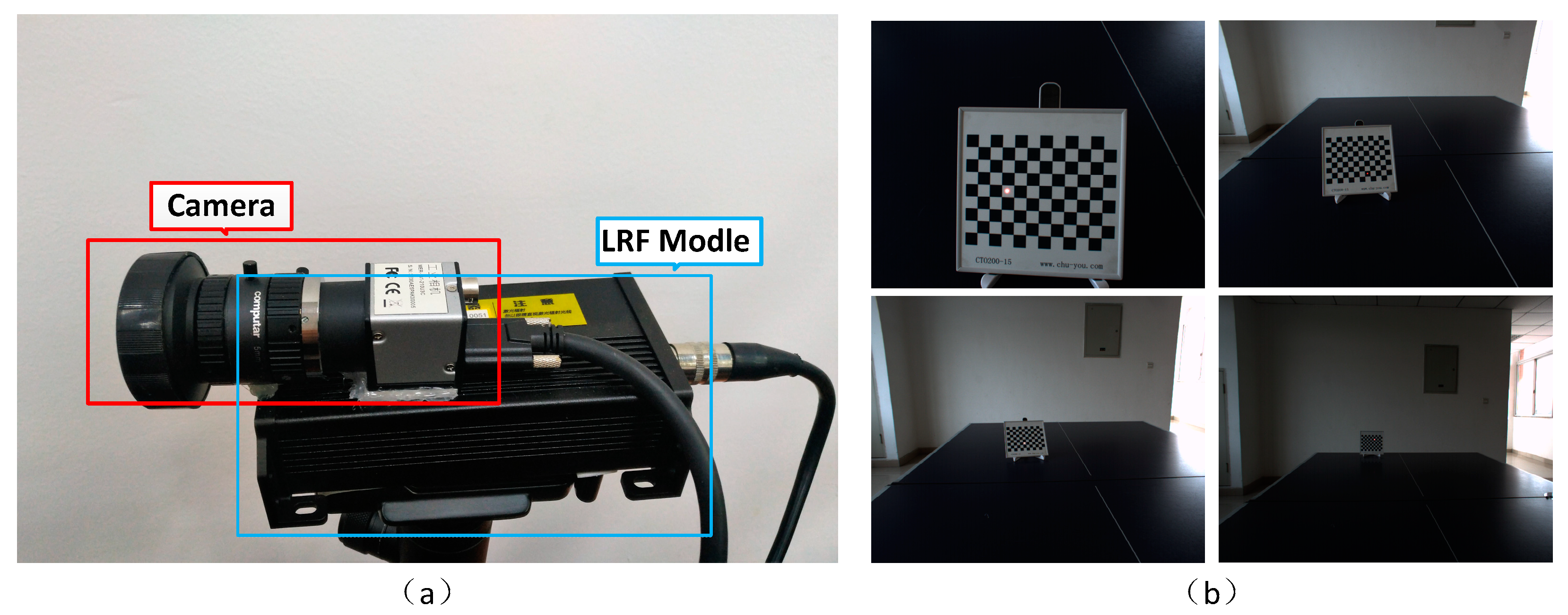
3.1. Initialization
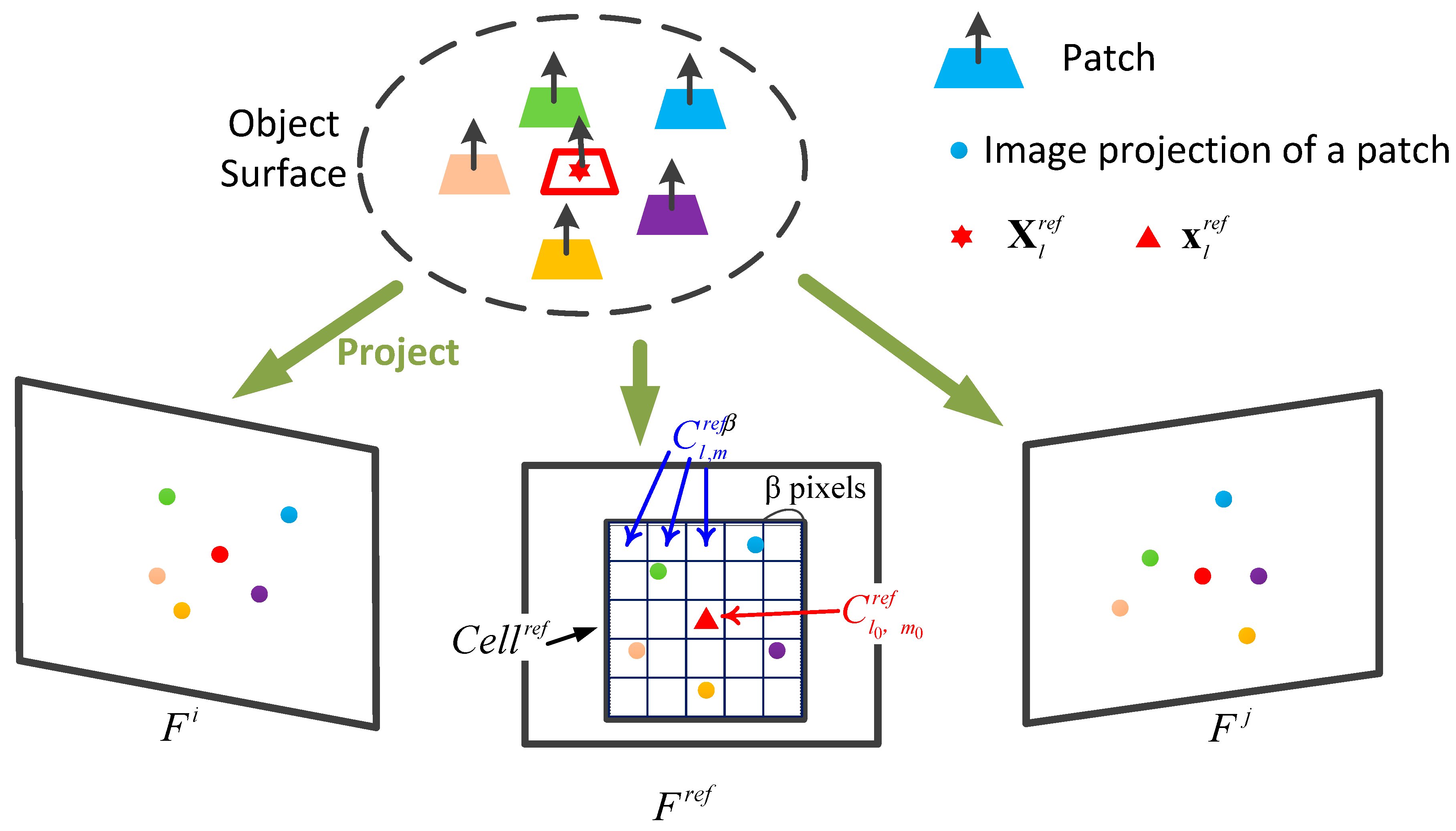
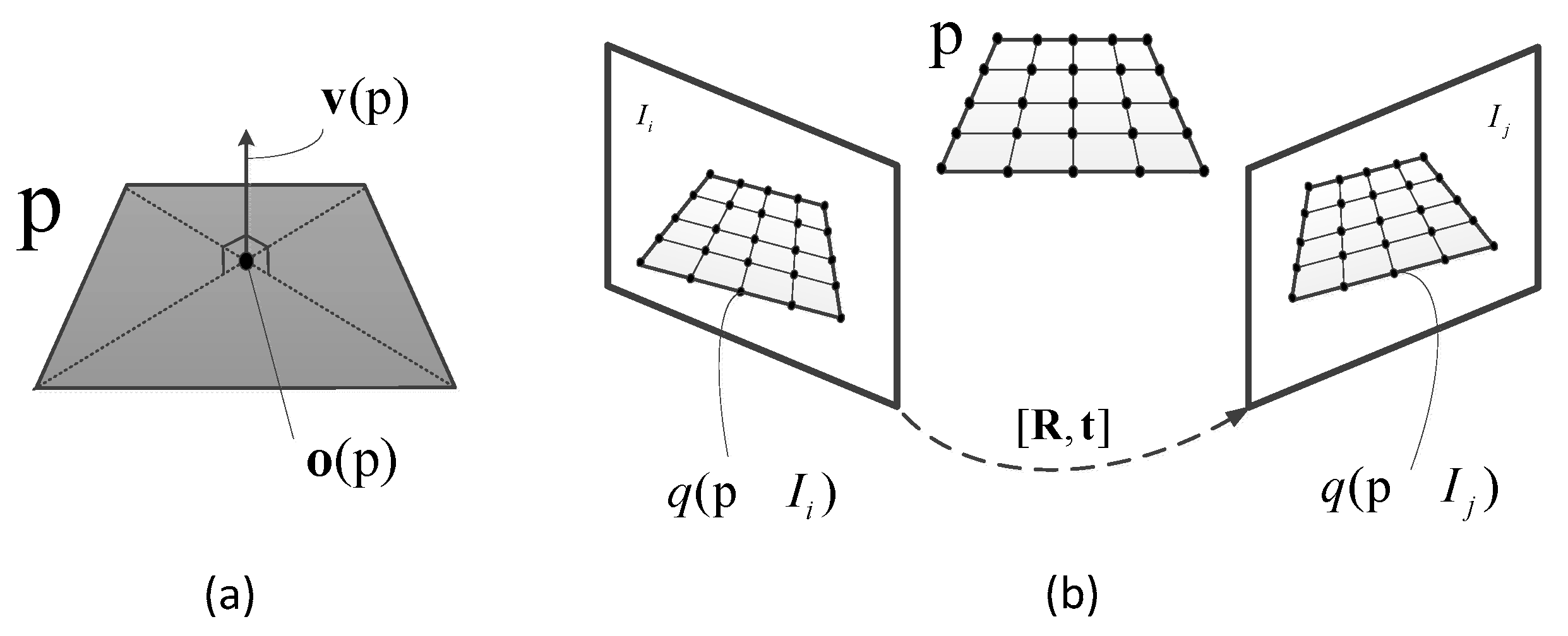
3.1.1. Initial Reconstruction
3.1.2. Patch Proliferation
3.1.3. Scale Estimation
3.2. Scale Correction
3.2.1. Drift Estimation
- (1)
- The scale of the last three estimates is offset by more than a certain amount relative to the current map scale:
- (2)
- The scale drift of the current image beam is still expanding:
- It is not necessary to update each KF cluster since the scale drift is relatively slow and an accurate scale could be followed for a long period.
- Too frequent updating scale takes up computing resources of the system and does not yield corresponding benefits.
- Although we effectively exclude the vast majority of wrong scale estimates, it cannot be rule out there will still be individual errors and frequent updates making the system less stable.
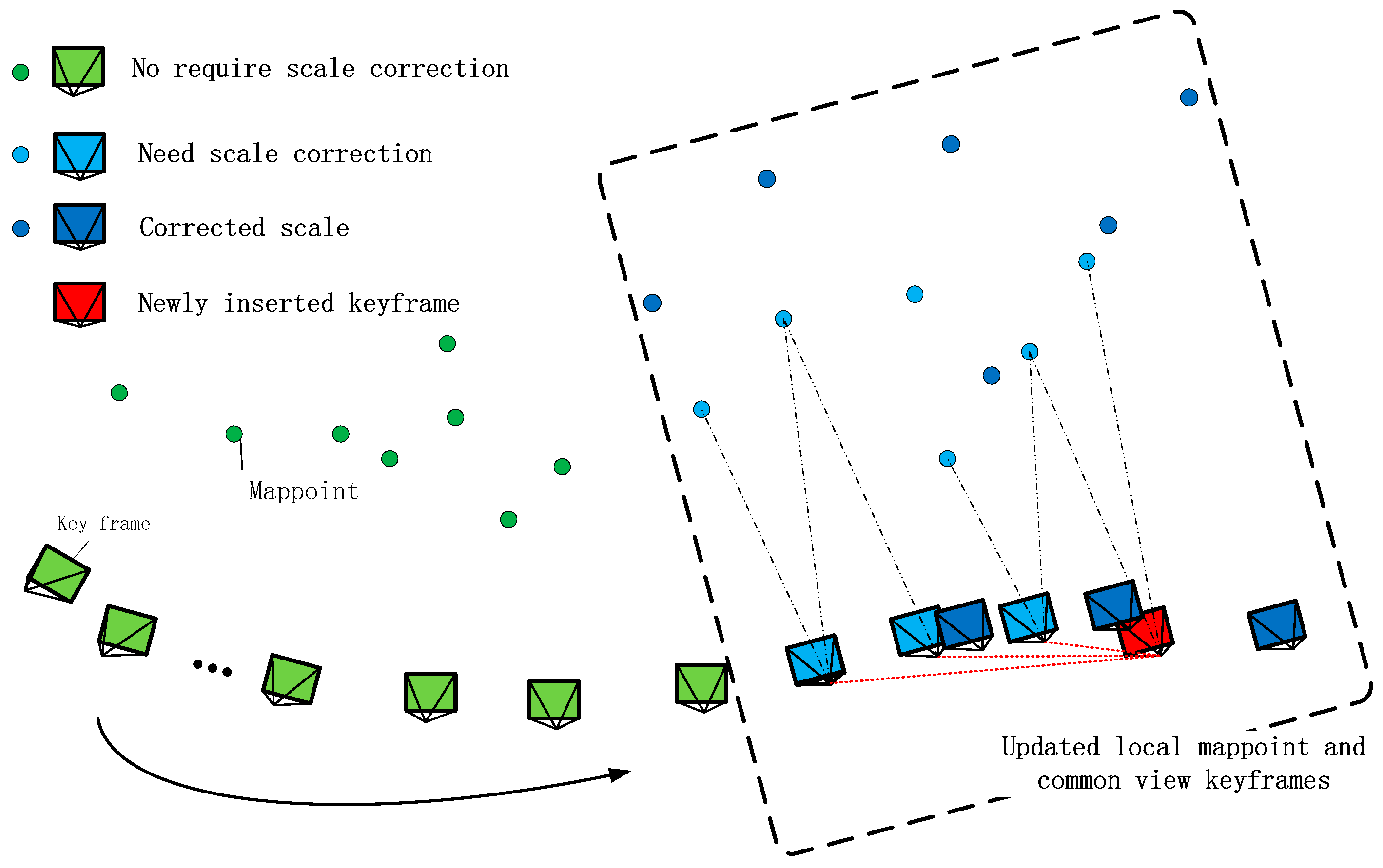
3.2.2. Scale Correction
- (1)
- Inserting a new key frame and enabling the local BA optimization process, the key frames, directly connected to the key frame, will be grouped into a KF-Bundle .
- (2)
- The map points observed by the key frames in the will be optimized.
- (3)
- All map points and key frames will be transformed in to the current local coordinate and will be re-scaled by .
- (4)
- Convert the local coordinates to the world coordinate and these information will be used for the following tracking.
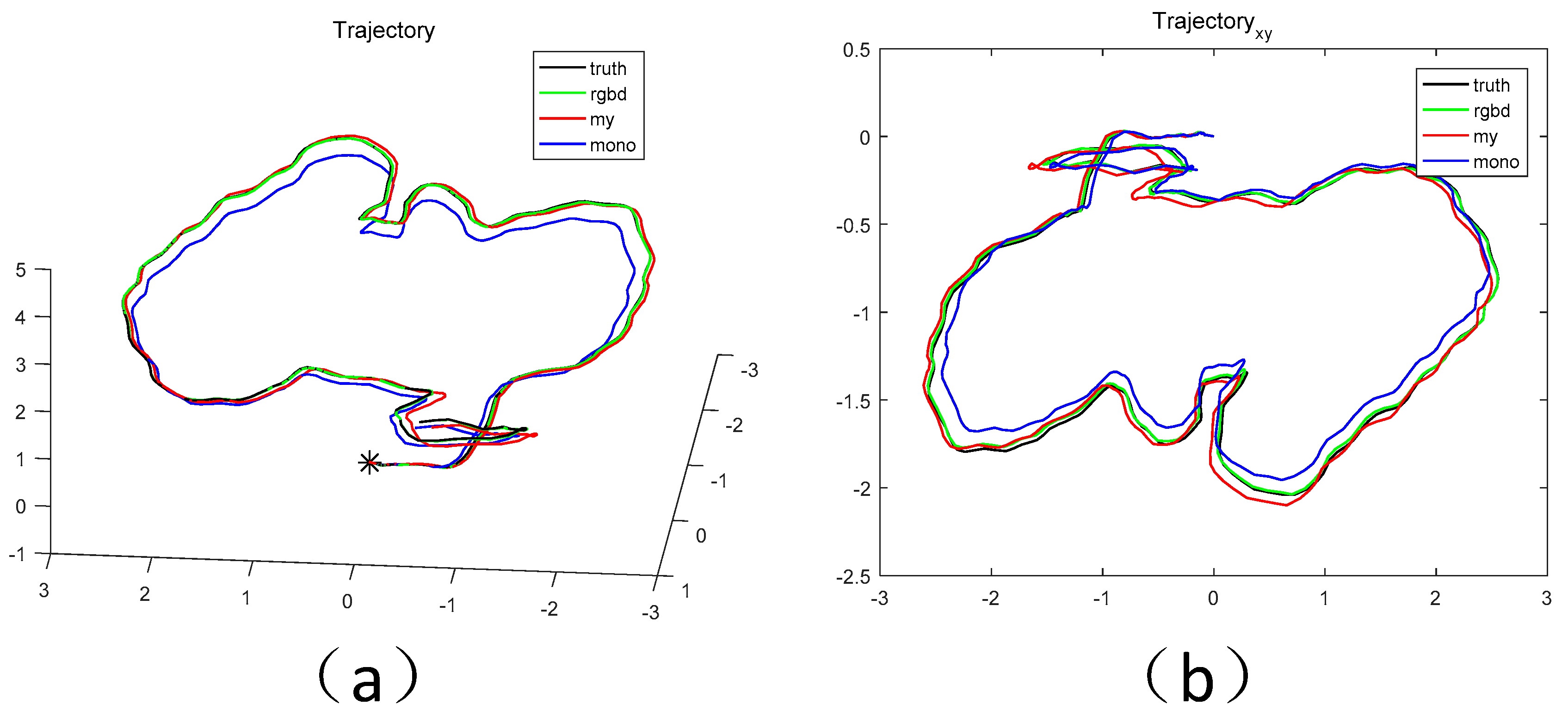
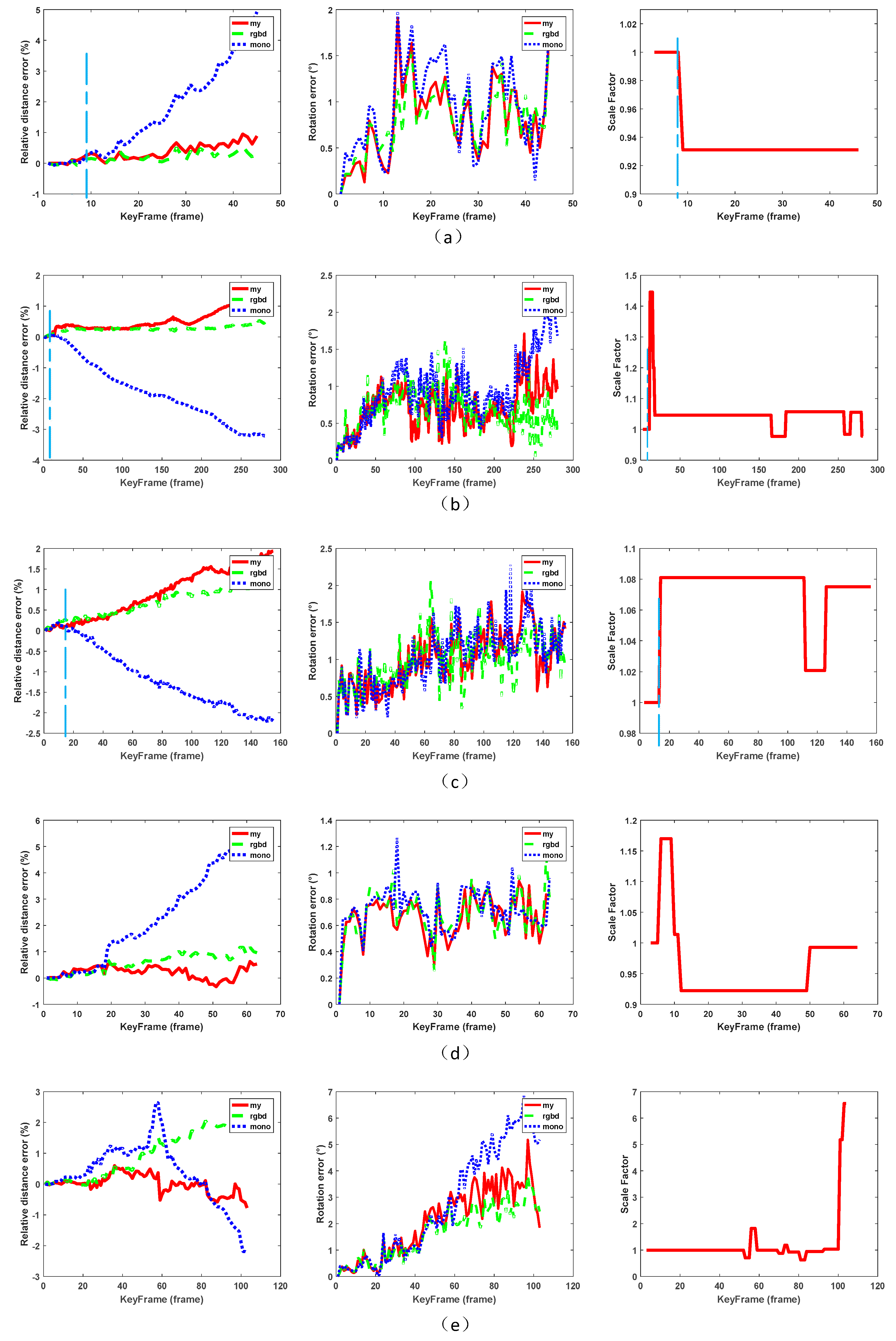
4. TUM Dataset Experiments
4.1. Initial Estimation
4.2. Scale Correction
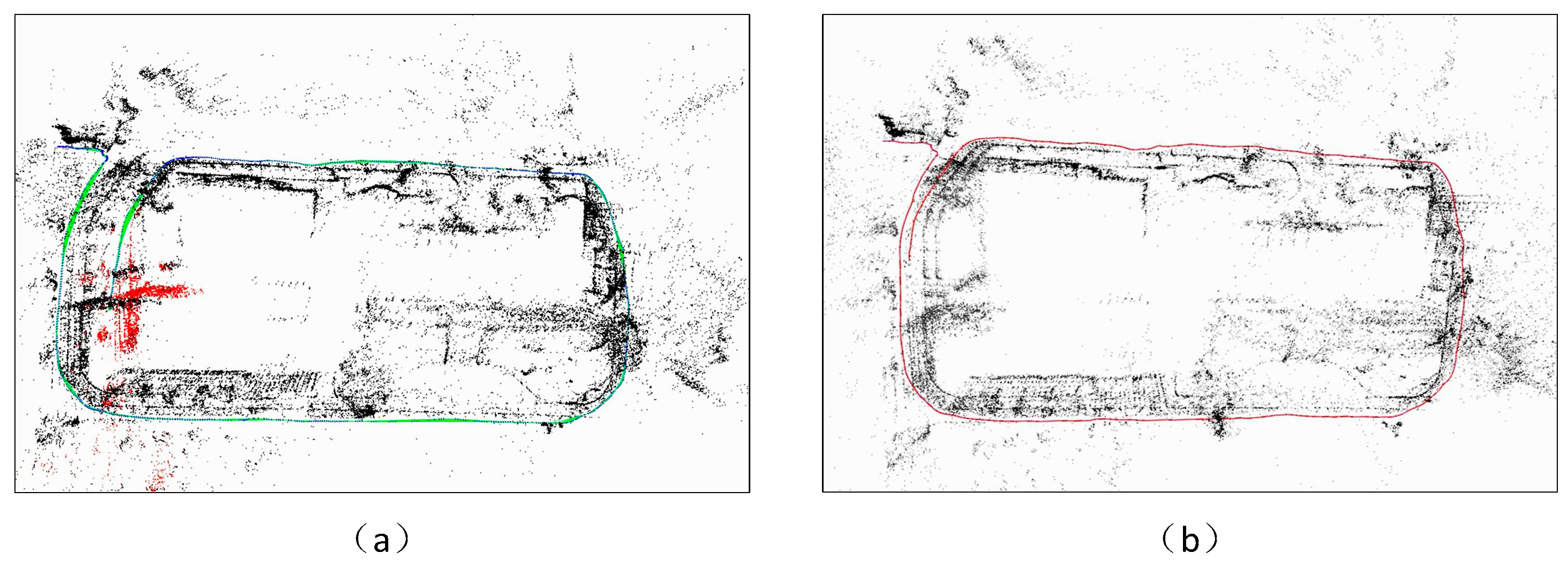
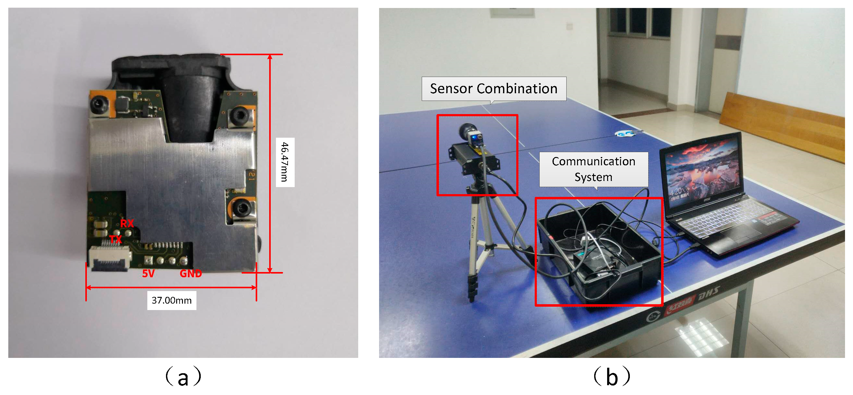
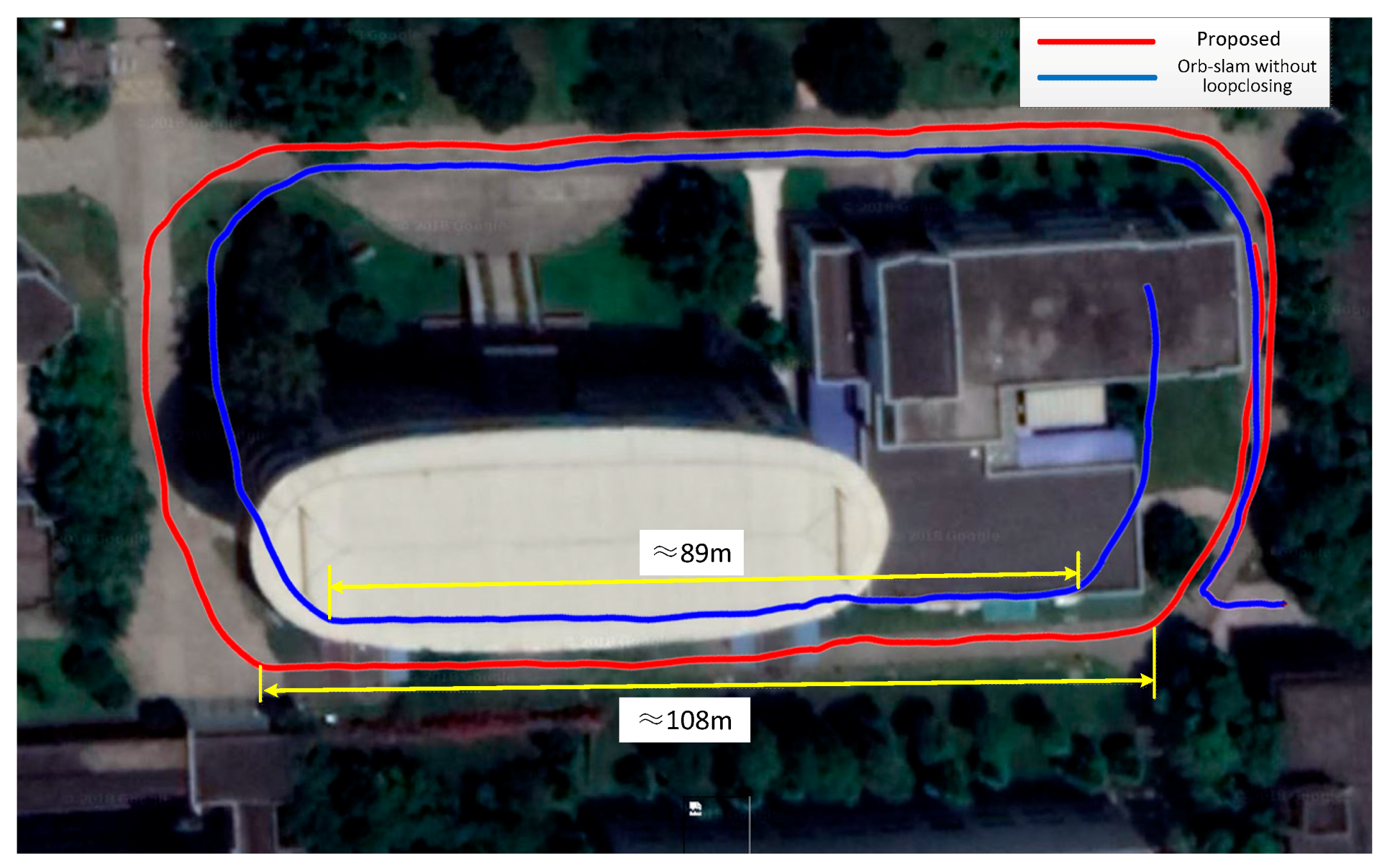
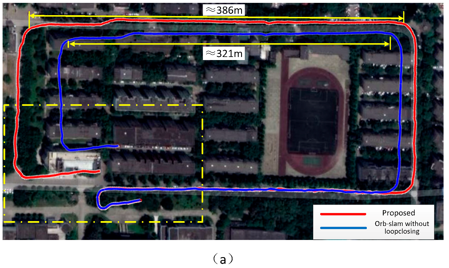
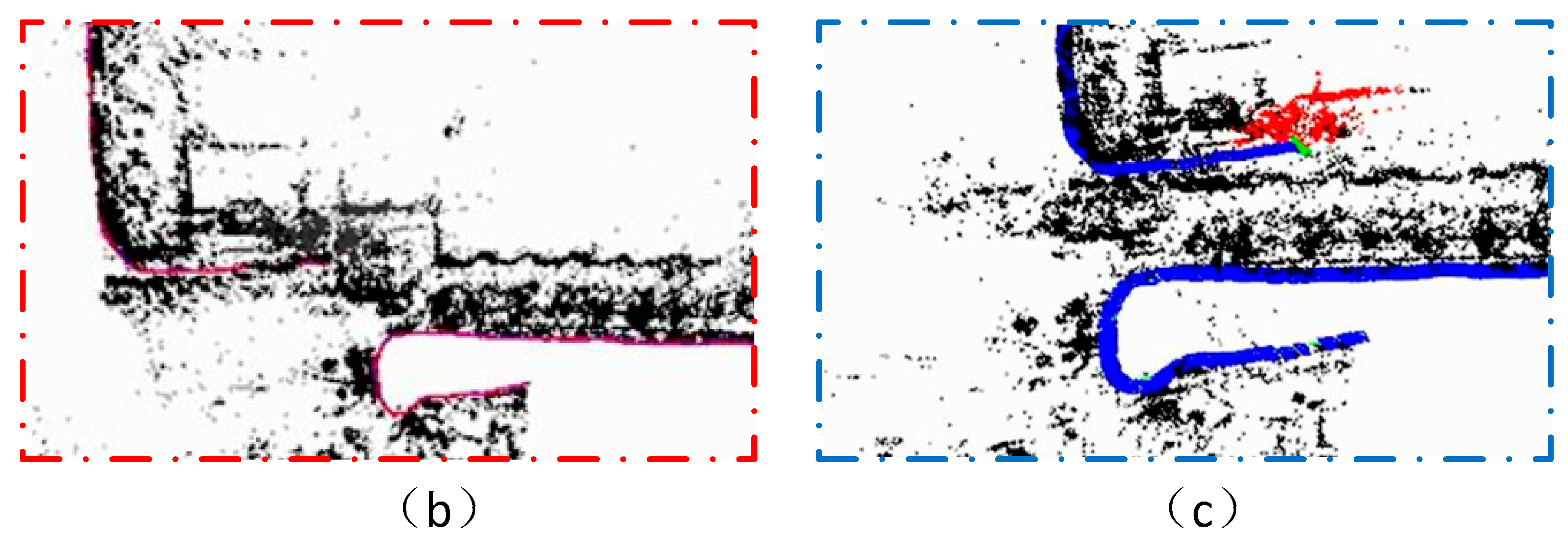
5. Self-Collected Dataset Experiments
5.1. Scene 1
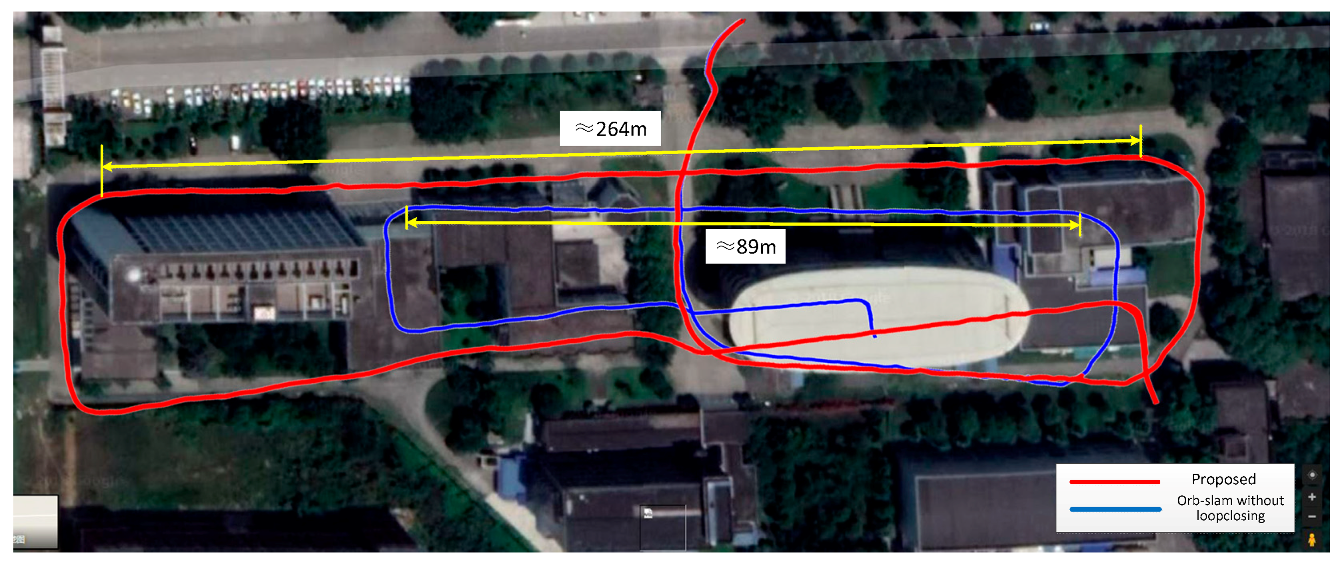
5.2. Scene 2
5.3. Scene 3
6. Conclusions
Author Contributions
Funding
Acknowledgments
Conflicts of Interest
Appendix A. The Normalized Cross Correlation (NCC) for Patch

References
- Davison, A. Real-time simultaneous localization and mapping with a single camera. In Proceedings of the Ninth IEEE International Conference on Computer Vision, Nice, France, 13–16 October 2003. [Google Scholar]
- Civera, J.; Davison, A.J.; Montiel, J.M.M. Inverse Depth Parametrization. In Structure from Motion using the Extended Kalman Filter; Springer: Heidelberg, Germany, 2012. [Google Scholar]
- Mur-Artal, R.; Tard, S.J.D. Orb-Slam2: An Open-Source Slam System for Monocular, Stereo, and RGB-D Cameras. IEEE Trans. Robot. 2017, 33, 1255–1262. [Google Scholar] [CrossRef]
- Mur-Artal, R.; Montiel, J.M.M.; Tard, S.J.D. Orb-Slam: A Versatile and Accurate Monocular SLAM System. IEEE Trans. Robot. 2015, 31, 1147–1163. [Google Scholar] [CrossRef]
- Engel, J.; Sch, P.S.T.; Cremers, D. Lsd-Slam: Large-Scale Direct Monocular SLAM. In Proceedings of the European Conference on Computer Vision, Zurich, Switzerland, 6–12 September 2014. [Google Scholar]
- Sturm, J.; Engelhard, N.; Endres, F.; Burgard, W.; Cremers, D. A benchmark for the evaluation of RGB-D SLAM systems. In Proceedings of the IEEE/RSJ International Conference on Intelligent Robots and Systems, Vilamoura, Portugal, 7–12 October 2012. [Google Scholar]
- Zhou, D.; Dai, Y.; Li, H. Reliable scale estimation and correction for monocular Visual Odometry. In Proceedings of the Intelligent Vehicles Symposium, Gothenburg, Sweden, 19–22 June 2016. [Google Scholar]
- Strasdat, H.; Davison, A.J.; Montiel, J.M.M.; Konolige, K. Double window optimisation for constant time visual SLAM. In Proceedings of the International Conference on Computer Vision, Barcelona, Spain, 6–13 November 2011. [Google Scholar]
- Carlone, L.; Aragues, R.; Castellanos, J.A.; Bona, B. A fast and accurate approximation for planar pose graph optimization. Int. J. Robot. Res. 2014, 33, 965–987. [Google Scholar] [CrossRef]
- Dubbelman, G.; Browning, B. Cop-Slam: Closed-Form Online Pose-Chain Optimization for Visual SLAM. IEEE Trans. Robot. 2015, 31, 1194–1213. [Google Scholar] [CrossRef]
- Civera, J.; Davison, A.J.; Montiel, J.M.M. Inverse Depth to Depth Conversion for Monocular SLAM. In Proceedings of the 2007 IEEE International Conference on Robotics and Automation, Roma, Italy, 10–14 April 2007; pp. 2778–2783. [Google Scholar]
- Civera, J.; Davison, A.J.; Montiel, J.M.M. Inverse Depth Parametrization for Monocular SLAM. IEEE Trans. Robot. 2008, 24, 932–945. [Google Scholar] [CrossRef] [Green Version]
- Scaramuzza, D.; Fraundorfer, F.; Pollefeys, M.; Siegwart, R. Absolute scale in structure from motion from a single vehicle mounted camera by exploiting nonholonomic constraints. In Proceedings of the IEEE International Conference on Computer Vision, Kyoto, Japan, 29 September–2 October 2009. [Google Scholar]
- Song, S.; Chandraker, M. Robust Scale Estimation in Real-Time Monocular SFM for Autonomous Driving. In Proceedings of the IEEE Conference on Computer Vision and Pattern Recognition, Columbus, OH, USA, 23–28 June 2014. [Google Scholar]
- Frost, D.P.; Kähler, O.; Murray, D.W. Object-aware bundle adjustment for correcting monocular scale drift. In Proceedings of the IEEE International Conference on Robotics and Automation, Stockholm, Sweden, 16–21 May 2016. [Google Scholar]
- Salas, M.; Montiel, J.M.M. Real-time monocular object SLAM. Robot. Auton. Syst. 2016, 75, 435–449. [Google Scholar] [Green Version]
- Dame, A.; Prisacariu, V.A.; Ren, C.Y.; Reid, I. Dense Reconstruction Using 3D Object Shape Priors. In Proceedings of the IEEE Conference on Computer Vision and Pattern Recognition, Portland, OR, USA, 23–28 June 2013. [Google Scholar]
- Botterill, T.; Mills, S.; Green, R. Correcting scale drift by object recognition in single-camera SLAM. IEEE Trans. Cybern. 2013, 43, 1767–1780. [Google Scholar] [CrossRef] [PubMed]
- Liu, F.; Shen, C.; Lin, G. Deep convolutional neural fields for depth estimation from a single image. In Proceedings of the 2015 IEEE Conference on Computer Vision and Pattern Recognition (CVPR), Boston, MA, USA, 7–12 June 2015; pp. 5162–5170. [Google Scholar]
- Eigen, D.; Fergus, R. Predicting Depth, Surface Normals and Semantic Labels with a Common Multi-scale Convolutional Architecture. In Proceedings of the 2015 IEEE International Conference on Computer Vision (ICCV), Santiago, Chile, 7–13 December 2015; pp. 2650–2658. [Google Scholar]
- Gao, X.; Zhang, T. Unsupervised learning to detect loops using deep neural networks for visual SLAM system. Auton. Robot. 2017, 41, 1–18. [Google Scholar] [CrossRef]
- Laina, I.; Rupprecht, C.; Belagiannis, V.; Tombari, F.; Navab, N. Deeper Depth Prediction with Fully Convolutional Residual Networks. In Proceedings of the 2016 Fourth International Conference on 3D Vision (3DV), Stanford, CA, USA, 25–28 October 2016; pp. 239–248. [Google Scholar]
- Tateno, K.; Tombari, F.; Laina, I.; Navab, N. CNN-Slam: Real-time dense monocular SLAM with learned depth prediction. In Proceedings of the 2017 IEEE Conference on Computer Vision and Pattern Recognition (CVPR), Honolulu, HI, USA, 21–26 July 2017; pp. 6565–6574. [Google Scholar]
- Martinelli, A. Vision and IMU Data Fusion: Closed-Form Solutions for Attitude, Speed, Absolute Scale, and Bias Determination. IEEE Trans. Robot. 2012, 28, 44–60. [Google Scholar] [CrossRef]
- Weiss, S.; Scaramuzza, D.; Siegwart, R. Fusion of IMU and Vision for Absolute Scale Estimation in Monocular SLAM. J. Intell. Robot. Syst. 2011, 61, 287–299. [Google Scholar]
- Wang, D.; Pan, Q.; Zhao, C.; Hu, J.; Liu, L.; Tian, L. SLAM-based cooperative calibration for optical sensors array with GPS/IMU aided. In Proceedings of the International Conference on Unmanned Aircraft Systems, Arlington, VA, USA, 7–10 June 2016. [Google Scholar]
- Shepard, D.P.; Humphreys, T.E. High-precision globally-referenced position and attitude via a fusion of visual SLAM, carrier-phase-based GPS, and inertial measurements. In Proceedings of the Position, Location and Navigation Symposium—PLANS 2014, Monterey, CA, USA, 5–8 May 2014. [Google Scholar]
- López, E.; García, A.S.; Barea, R.; Bergasa, L.M.; Molinos, E.J.; Arroyo, R.; Romera, E.; Pardo, S. A Multi-Sensorial Simultaneous Localization and Mapping (SLAM) System for Low-Cost Micro Aerial Vehicles in GPS-Denied Environments. Sensors 2017, 17, 802. [Google Scholar] [CrossRef] [PubMed]
- Zhang, J.; Singh, S.; Kantor, G. Robust Monocular Visual Odometry for a Ground Vehicle in Undulating Terrain. Field Serv. Robot. 2012, 92, 311–326. [Google Scholar]
- Valiente, D.; Gil, A.; Reinoso, Ó.; Juliá, M.; Holloway, M. Improved Omnidirectional Odometry for a View-Based Mapping Approach. Sensors 2017, 17, 325. [Google Scholar] [CrossRef] [PubMed]
- Valiente, D.; Gil, A.; Payá, L.; Sebastián, J.M.; Reinoso, Ó. Robust Visual Localization with Dynamic Uncertainty Management in Omnidirectional SLAM. Appl. Sci. 2017, 7, 1294. [Google Scholar] [CrossRef]
- Engel, J.; Stückler, J.; Cremers, D. Large-scale direct SLAM with stereo cameras. In Proceedings of the IEEE/RSJ International Conference on Intelligent Robots and Systems, Hamburg, Germany, 28 September–2 October 2015. [Google Scholar]
- Geiger, A.; Ziegler, J.; Stiller, C. StereoScan: Dense 3D reconstruction in real-time. In Proceedings of the Intelligent Vehicles Symposium, Baden-Baden, Germany, 5–9 June 2011. [Google Scholar]
- Tian, J.D.; Sun, J.; Tang, Y.D. Short-Baseline Binocular Vision System for a Humanoid Ping-Pong Robot. J. Intell. Robot. Syst. 2011, 64, 543–560. [Google Scholar] [CrossRef] [Green Version]
- Zhang, L.; Shen, P.; Zhu, G.; Wei, W.; Song, H. A Fast Robot Identification and Mapping Algorithm Based on Kinect Sensor. Sensors 2015, 15, 19937–19967. [Google Scholar] [CrossRef] [PubMed] [Green Version]
- Di, K.; Qiang, Z.; Wan, W.; Wang, Y.; Gao, Y. RGB-D SLAM Based on Extended Bundle Adjustment with 2D and 3D Information. Sensors 2016, 16, 1285. [Google Scholar] [CrossRef] [PubMed]
- Henry, P.; Krainin, M.; Herbst, E.; Ren, X.; Fox, D. RGB-D Mapping: Using Kinect-Style Depth Cameras for Dense 3D Modeling of Indoor Environments. Int. J. Robot. Res. 2012, 31, 647–663. [Google Scholar] [CrossRef]
- Endres, F.; Hess, J.; Sturm, J.; Cremers, D.; Burgard, W. 3-D Mapping With an RGB-D Camera. IEEE Trans. Robot. 2017, 30, 177–187. [Google Scholar] [CrossRef]
- Burgard, W.; Engelhard, N.; Endres, F.; Hess, J.; Sturm, J. Real-time 3D visual SLAM with a hand-held RGB-D camera. In Proceedings of the RGB-D Workshop on 3D Perception in Robotics at the European Robotics Forum, Västerås, Sweden, 8 April 2011. [Google Scholar]
- Pollefeys, M. Multiple View Geometry. In Encyclopedia of Biometrics; Springer: Berlin, Germany, 2005; Volume 2, pp. 181–186. [Google Scholar]
- Furukawa, Y. Multi-View Stereo: A Tutorial; Now Publishers Inc.: Breda, The Netherlands, 2015. [Google Scholar]
- Rublee, E.; Rabaud, V.; Konolige, K.; Bradski, G. ORB: An efficient alternative to SIFT or SURF. In Proceedings of the International Conference on Computer Vision, Barcelona, Spain, 6–13 November 2011. [Google Scholar]
- Argyros, A. The Design and Implementation of a Generic Sparse Bundle Adjustment Software Package Based on the LM Algorithm; FORTH-ICS Technical Report; Institute of Computer Science-FORTH: Crete, Greece, 2004. [Google Scholar]
- Lepetit, V.; Moreno-Noguer, F.; Fua, P. EPnP: An Accurate O(n) Solution to the PnP Problem. Int. J. Comput. Vis. 2009, 81, 155–166. [Google Scholar] [CrossRef] [Green Version]


| Scene | Data | Proposed Method | RGBD | Monocular | ||
|---|---|---|---|---|---|---|
| Number | Err (%) | Number | Err (%) | Number | ||
| Testing | fr1/xyz | 185 | 1.30 | 1 | 0.11 | 177 |
| Handheld SLAM | fr3/office | 41 | 5.51 | 1 | 0.64 | 26 |
| No structure | fr3/near | 59 | 4.46 | 1 | 0.54 | 53 |
| Dynamic objects | fr3/xyz | 68 | 4.21 | 1 | 0.86 | 56 |
| 3D Reconstruction | fr1/teddy | 13 | 3.66 | 1 | 0.61 | 7 |
| Scenarios | Frames Number | GPS | Proposed Method | Monocular |
|---|---|---|---|---|
| 1 | 8871 | 407 (m) | 405 (m) | 348 (m) |
| 2 | 12,787 | 1.23 (km) | 1.17 (km) | 954 (m) |
| 3 | 9921 | 959 (m) | 913 (m) | 607 (m) |
© 2018 by the authors. Licensee MDPI, Basel, Switzerland. This article is an open access article distributed under the terms and conditions of the Creative Commons Attribution (CC BY) license (http://creativecommons.org/licenses/by/4.0/).
Share and Cite
Zhang, Z.; Zhao, R.; Liu, E.; Yan, K.; Ma, Y. Scale Estimation and Correction of the Monocular Simultaneous Localization and Mapping (SLAM) Based on Fusion of 1D Laser Range Finder and Vision Data. Sensors 2018, 18, 1948. https://doi.org/10.3390/s18061948
Zhang Z, Zhao R, Liu E, Yan K, Ma Y. Scale Estimation and Correction of the Monocular Simultaneous Localization and Mapping (SLAM) Based on Fusion of 1D Laser Range Finder and Vision Data. Sensors. 2018; 18(6):1948. https://doi.org/10.3390/s18061948
Chicago/Turabian StyleZhang, Zhuang, Rujin Zhao, Enhai Liu, Kun Yan, and Yuebo Ma. 2018. "Scale Estimation and Correction of the Monocular Simultaneous Localization and Mapping (SLAM) Based on Fusion of 1D Laser Range Finder and Vision Data" Sensors 18, no. 6: 1948. https://doi.org/10.3390/s18061948