Automatic Identification of Alpine Mass Movements by a Combination of Seismic and Infrasound Sensors


Abstract
1. Introduction
2. Detection System
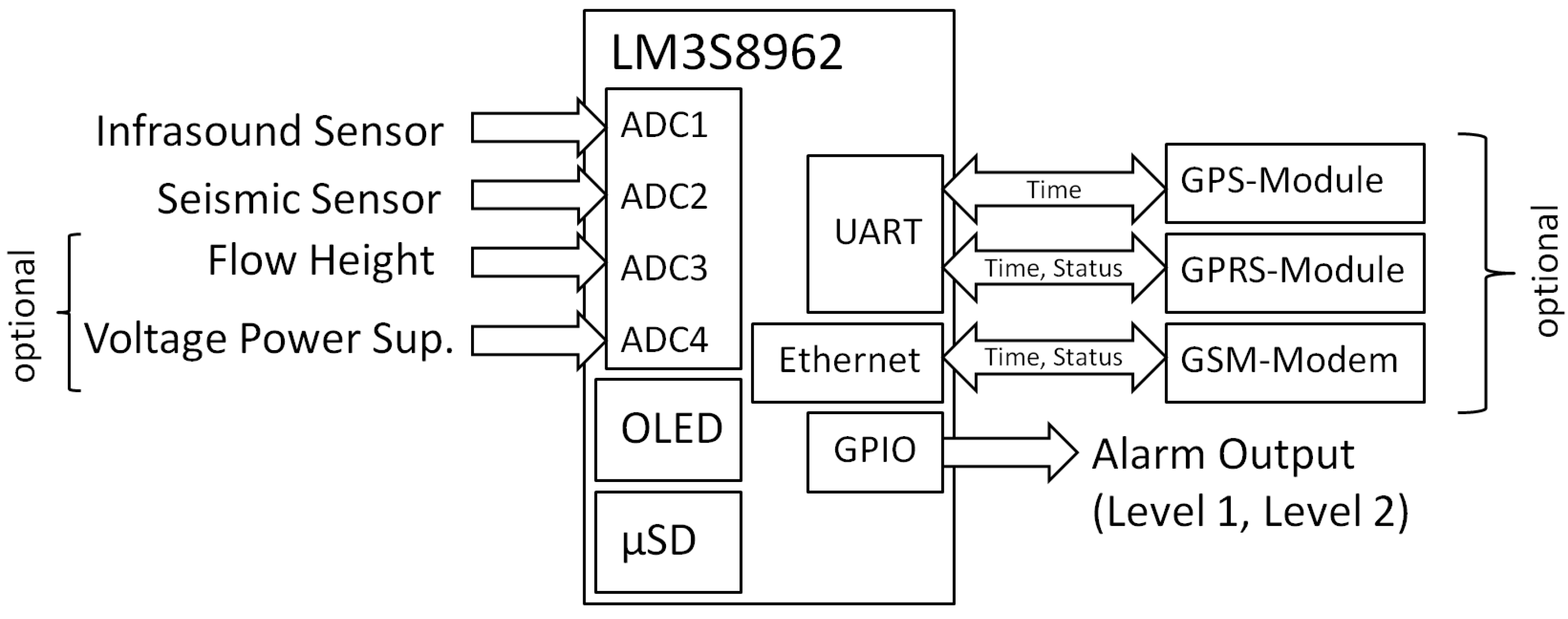
2.1. Hardware Setup
2.2. Software Design
2.3. Detection Algorithm
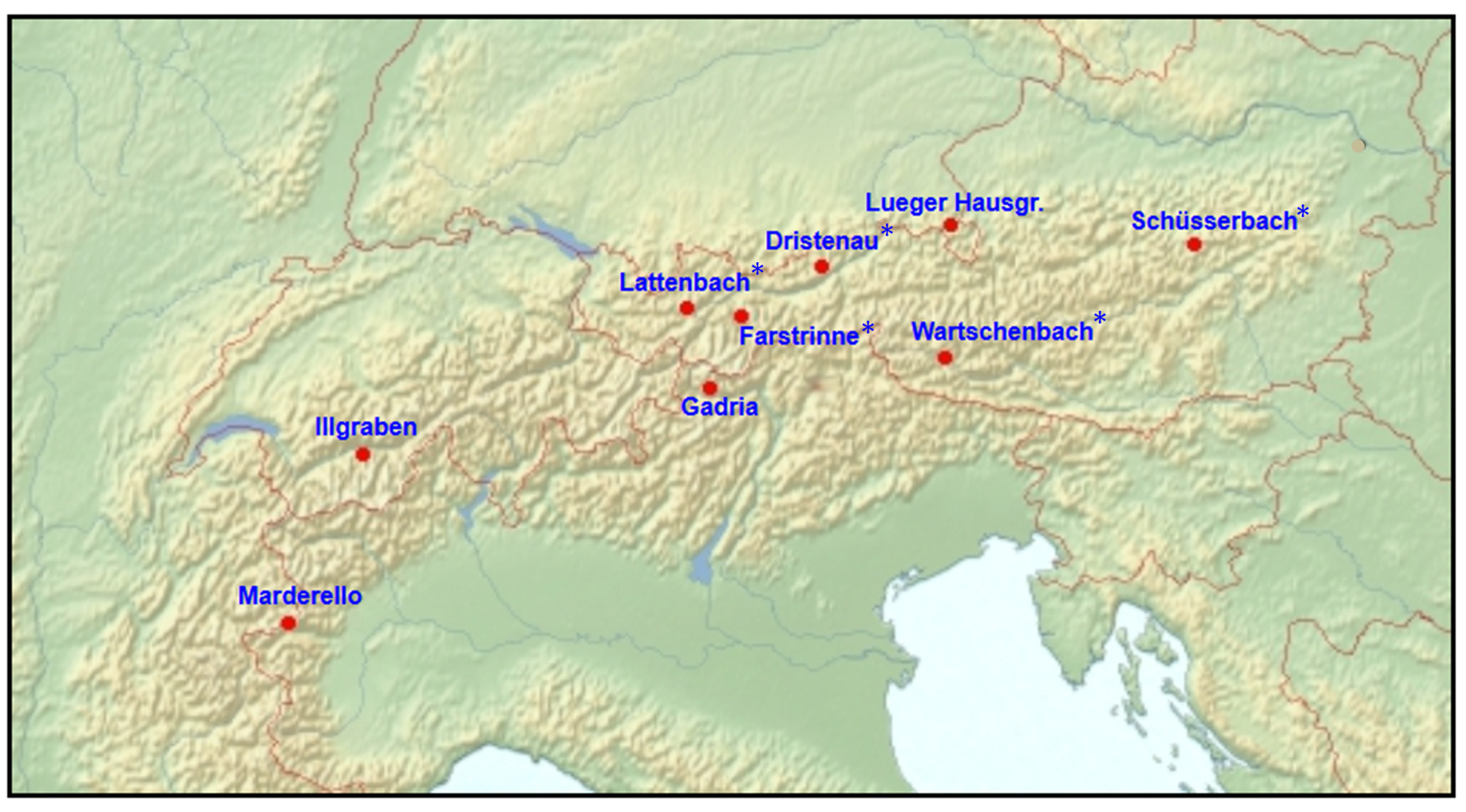
3. Test Sites
4. Example Events
4.1. Marderello
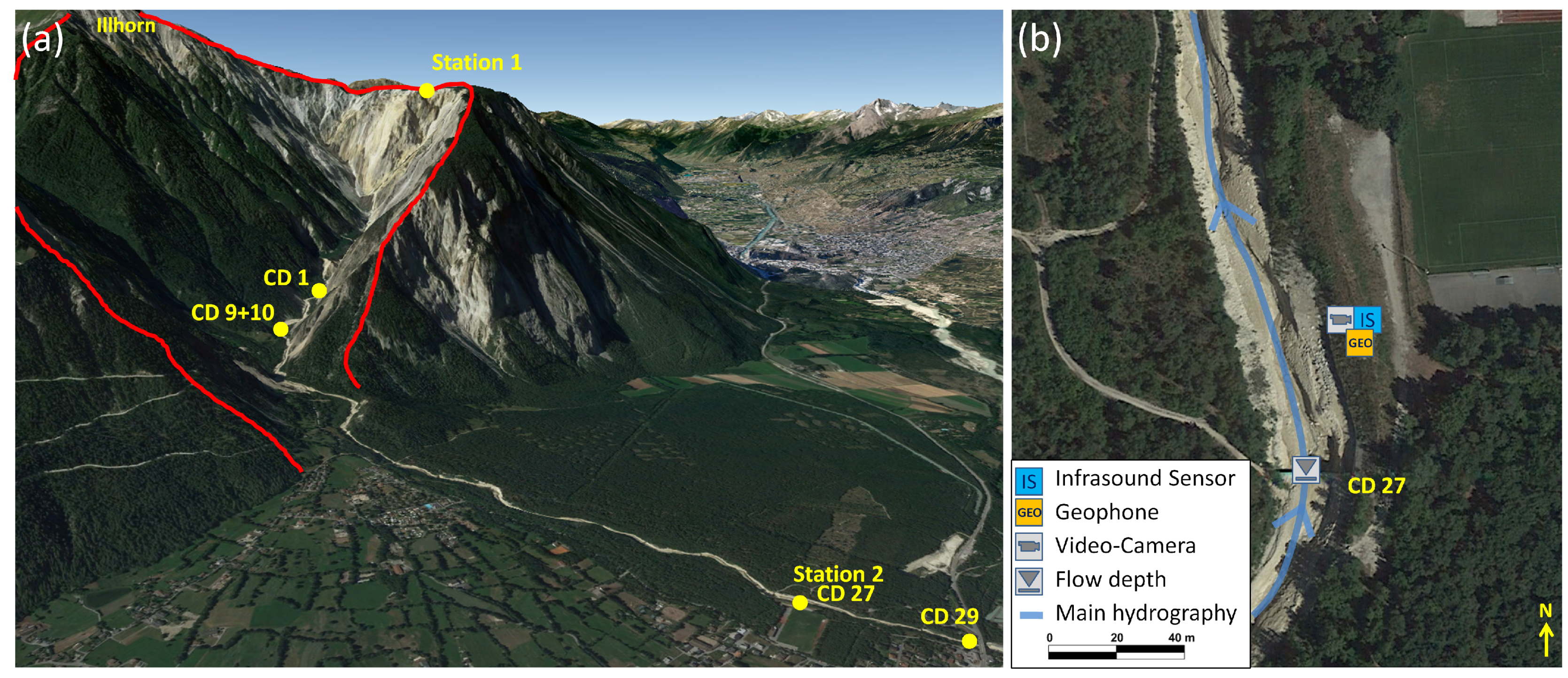
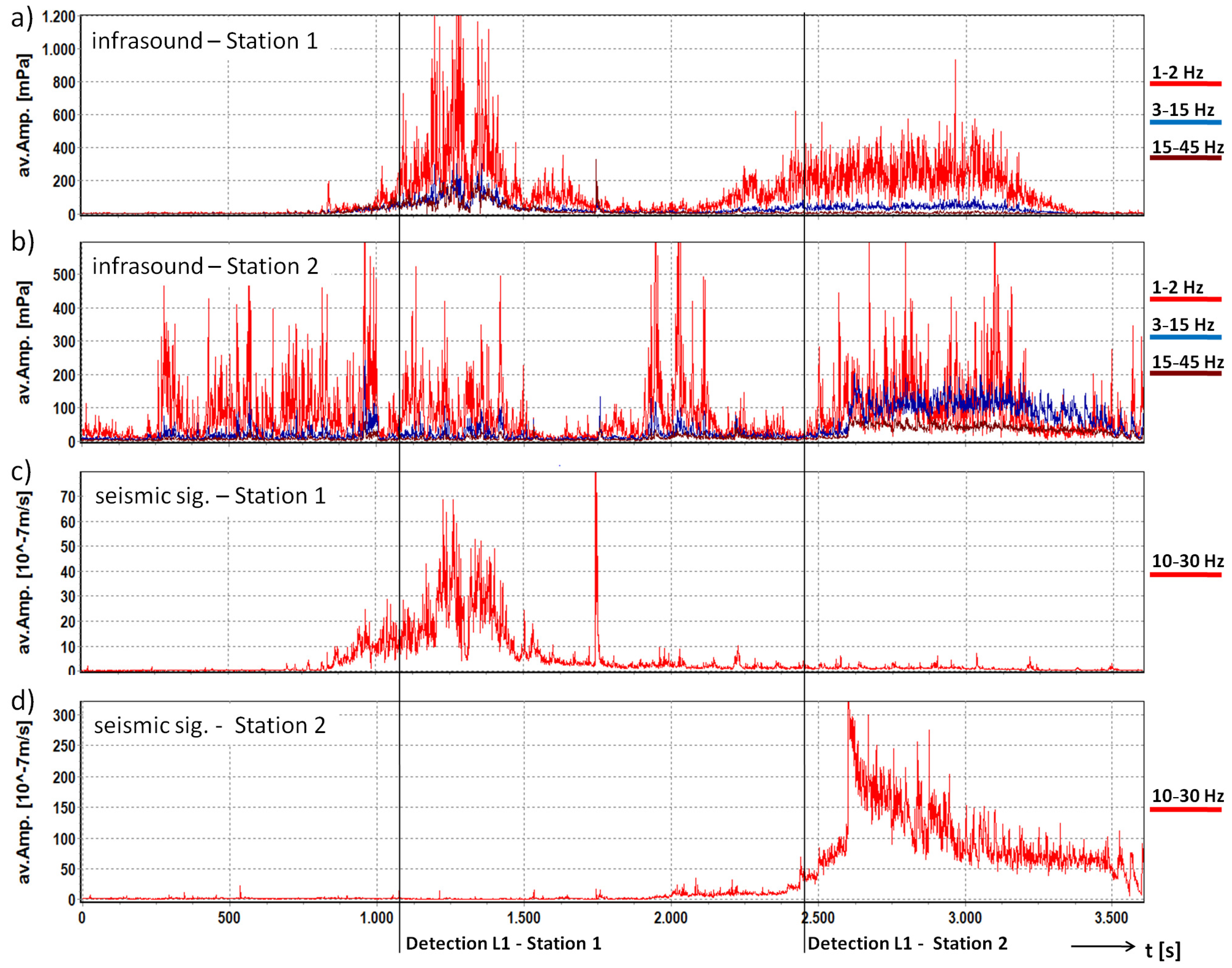
4.2. Illgraben
5. Results and Discussion
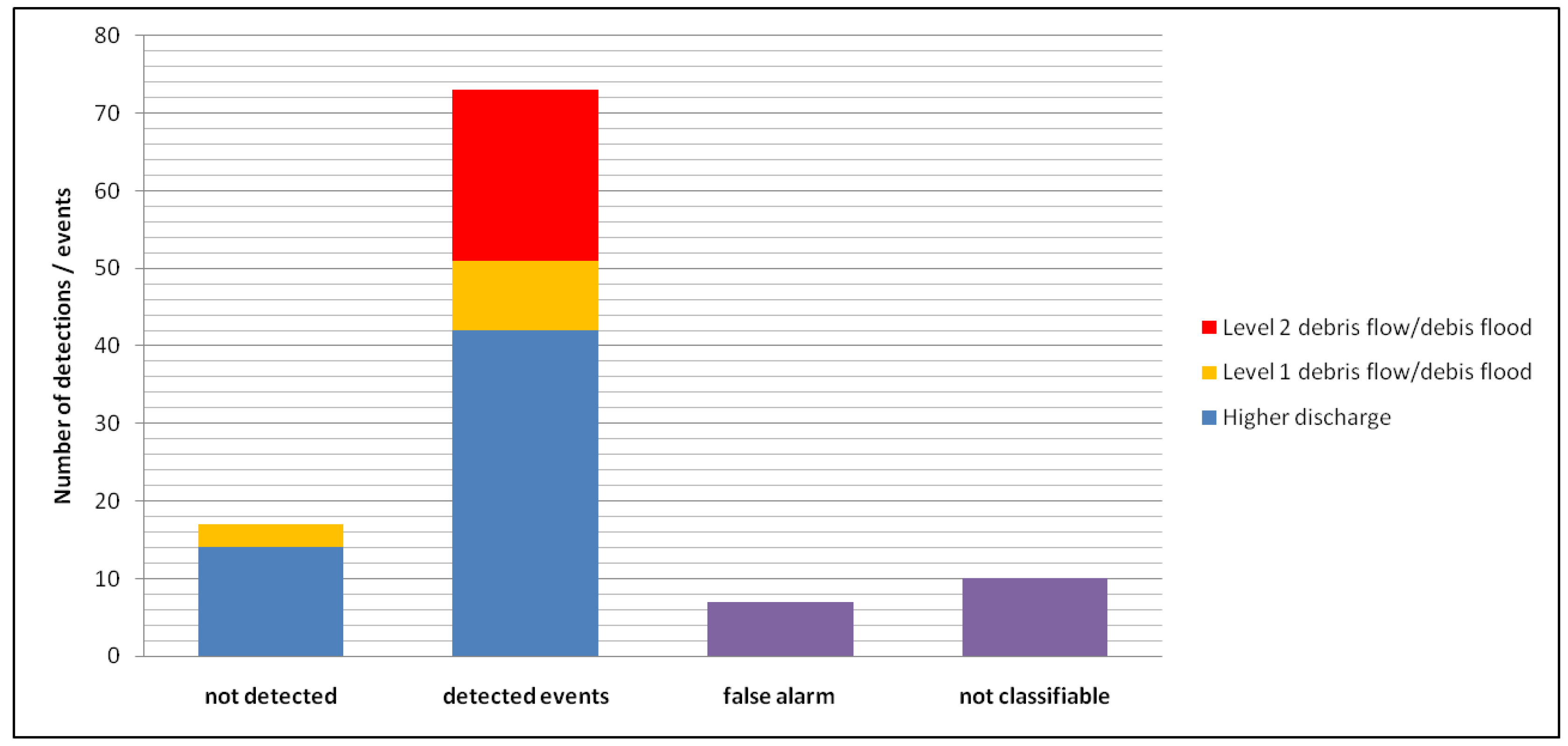
5.1. Evaluation of the Detection Algorithm
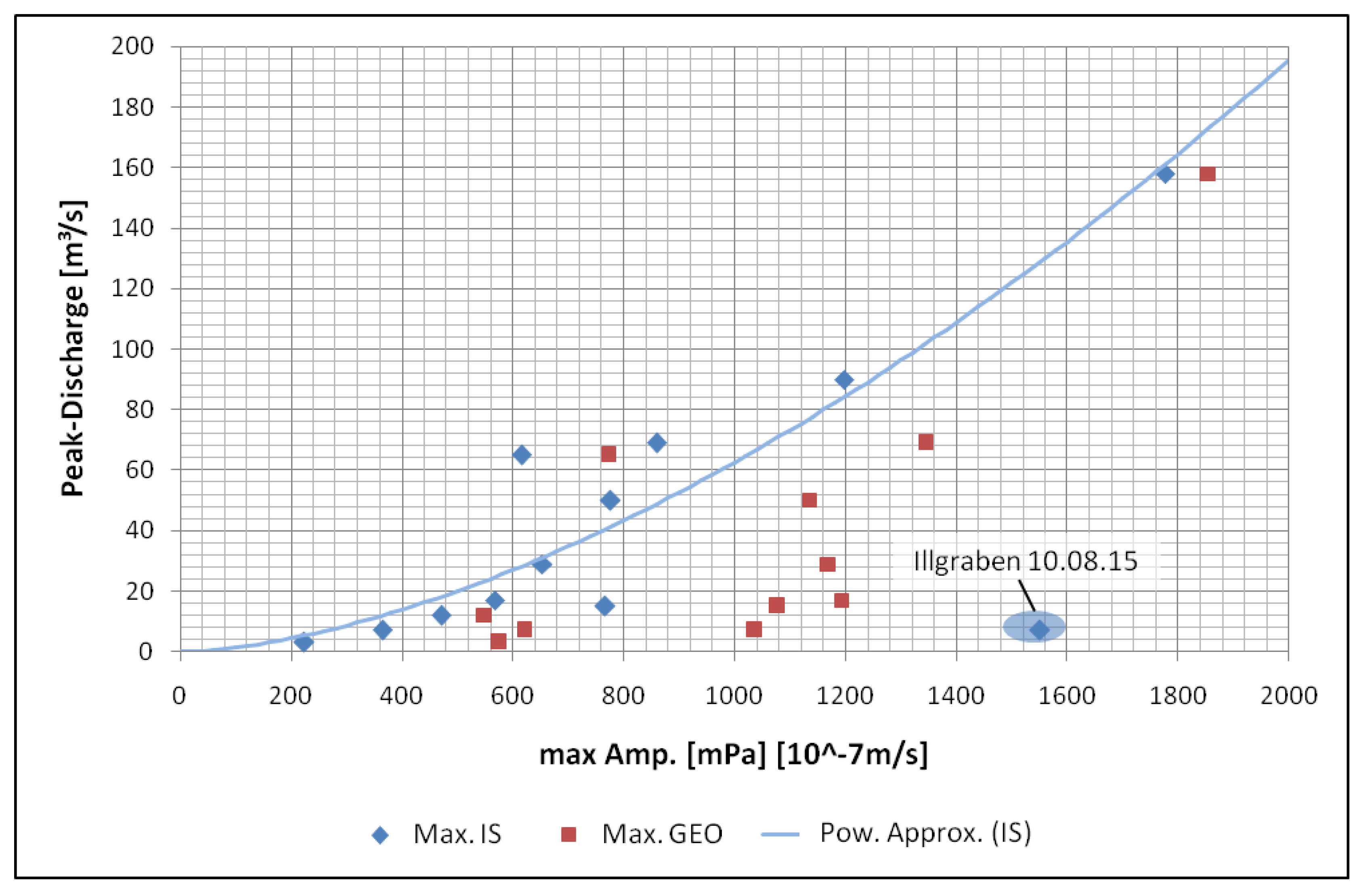
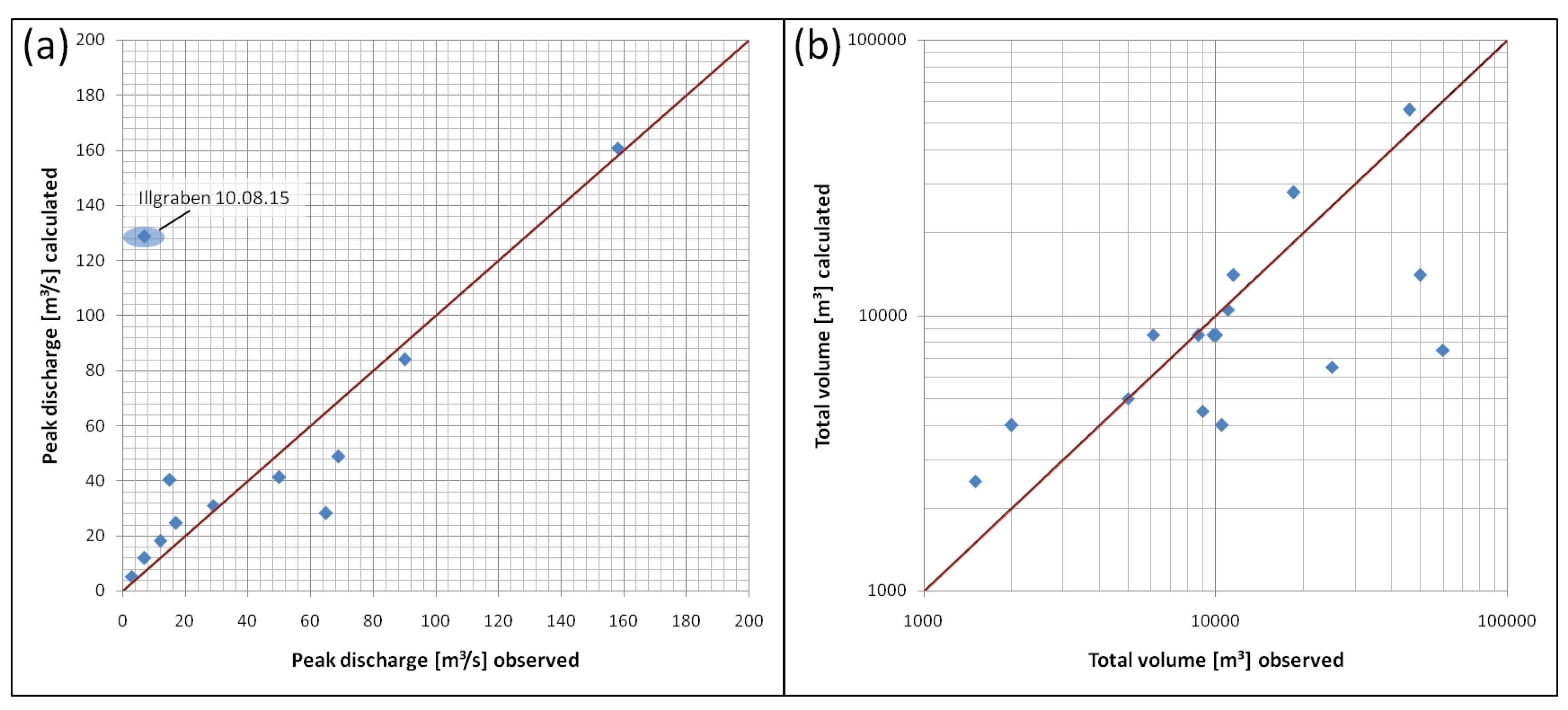
5.2. Magnitude Estimation
6. Conclusions
Author Contributions
Acknowledgments
Conflicts of Interest
References
- Hunger, O.; Evans, S.G.; Bovis, M.J.; Hutchinson, J.N. A review of the classification of landslides of the flow type. Environ. Eng. Geosci. 2001, 7, 221–238. [Google Scholar] [CrossRef]
- Coussot, P.; Laigle, D.; Arattano, M.; Deganutti, A.M.; Marchi, L. Direct determination of rheological characteristics of debris flow. J. Hydraul. Eng. 1998, 124, 865–868. [Google Scholar] [CrossRef]
- Kean, J.W.; Coe, J.A.; Coviello, V.; Smith, J.B.; McCoy, S.W.; Arattano, M. Estimating rates of debris flow entrainment from ground vibrations. Geophys. Res. Lett. 2015, 42, 6365–6372. [Google Scholar] [CrossRef]
- Tsai, V.C.; Minchew, B.; Lamb, M P.; Ampuero, J.P. A physical model for seismic noise generation from sediment transport in rivers. Geophys. Res. Lett. 2012, 39, 1944–8007. [Google Scholar] [CrossRef]
- Biescas, B.; Dufour, F.; Furdada, G.; Khazaradze, G.; Suriñach, E. Frequency content evolution of snow avalanche seismic signals. Surv. Geophys. 2003, 24, 447–464. [Google Scholar] [CrossRef]
- Huang, C.-J.; Yin, H.-Y.; Chen, C.-Y.; Yeh, C.-H.; Wang, C.-L. Ground vibrations produced by rock motions and debris flows. J. Geophys. Res. Earth Surf. 2007, 112, F02014. [Google Scholar] [CrossRef]
- Vilajosana, I.; Suriñach, E.; Abellán, A.; Khazaradze, G.; Garcia, D.; Llosa, J. Rockfall induced seismic signals: Case study in Montserrat, Catalonia. Nat. Hazards Earth Syst. Sci. 2008, 8, 805–812. [Google Scholar] [CrossRef]
- Arattano, M.; Marchi, L.; Cavalli, M. Analysis of debris-flow recordings in an instrumented basin: Confirmations and new findings. Nat. Hazards Earth Syst. Sci. 2012, 12, 679–686. [Google Scholar] [CrossRef]
- Arattano, M.; Abancó, C.; Coviello, V.; Hürlimann, M. Processing the ground vibration signal produced by debris flows: The methods of amplitude and impulses compared. Comput. Geosci. 2014, 73, 17–27. [Google Scholar] [CrossRef]
- Abancó, C.; Hürlimann, M.; Fritschi, B.; Graf, C.; Moya, J. Transformation of ground vibration signal for debris-flow monitoring and detection in alarm systems. Sensors 2012, 12, 4870–4891. [Google Scholar] [CrossRef] [PubMed]
- Coviello, V.; Arattano, M.; Turconi, L. Detecting torrential processes from a distance with a seismic monitoring network. Nat. Hazards 2015, 78, 2055–2080. [Google Scholar] [CrossRef]
- Walter, F.; Burtin, A.; McArdell, B.W.; Hovius, N.; Weder, B.; Turowski, J.M. Testing seismic amplitude source location for fast debris-flow detection at Illgraben, Switzerland. Nat. Hazards Earth Syst. Sci. 2017, 17, 939–955. [Google Scholar] [CrossRef]
- Chou, H.T.; Cheung, Y.L.; Zhang, S. Calibration of Infrasound Monitoring System and Acoustic Characteristics of Debris-Flow Movement by Field Studies. In Proceedings of the Fourth International Conference on Debris-Flow Hazards Mitigation: Mechanics, Prediction, and Assessment, Chengdu, China, 10–13 September 2007; Chen, C.L., Major, J.J., Eds.; Millpress: Rotterdam, The Netherlands, 2007; pp. 571–580. [Google Scholar]
- Kogelnig, A.; Hübl, J.; Suriñach, E.; Vilajosana, I.; McArdell, B.W. Infrasound produced by debris flow: Propagation and frequency content evolution. Nat. Hazards 2014, 70, 1713–1733. [Google Scholar] [CrossRef]
- Pilger, C.; Bittner, M. Infrasound from tropospheric sources: Impact on mesopause temperature? J. Atmos. Sol. Terr. Phys. 2009, 71, 816–822. [Google Scholar] [CrossRef]
- Kogelnig, A. Development of Acoustic Monitoring for Alpine Mass Movements. Ph.D. Thesis, University of Natural Resources and Life Sciences (BOKU), Institute of Mountain Risk Engineering, Vienna, Austria, 2012. [Google Scholar]
- Chou, H.T.; Chang, Y.L.; Zhang, S.X. Acoustic signals and geophone response of rainfall-induced debris flows. J. Chin. Inst. Eng. 2010, 36, 335–347. [Google Scholar] [CrossRef]
- Liu, D.; Leng, X.; Wei, F.; Zhang, S.; Hong, Y. Monitoring and recognition of debris flow infrasonic signals. J. Mt. Sci. 2015, 12, 797–815. [Google Scholar] [CrossRef]
- Suriñach, E.; Kogelnig, A.; Vilajosana, I.; Hübl, J.; Hiller, M.; Dufour, F. Incoporación del la señal de infrasonido a la detección y estudio de aludes de nieve y flujostorrenciales. In Proceedings of the VII Simposio Nacional sobre Taludes y Laderas Inestables, Barcelona, Spain, 27–30 October 2009. [Google Scholar]
- Hübl, J.; Schimmel, A.; Kogelnig, A.; Suriñach, E.; Vilajosana, I.; McArdell, B.W. A review on acoustic monitoring of debris flow. Int. J. Saf. Secur. Eng. 2013, 3, 105–115. [Google Scholar] [CrossRef]
- Leprette, B.; Martin, N.; Glangeaud, F.; Navarre, J.P. Three-component signal recognition using time, time-frequency, and polarization information-application to seismic detection of avalanches. IEEE Trans. Signal Process. 1998, 46, 83–102. [Google Scholar] [CrossRef]
- Bessason, B.; Eiríksson, G.; Thórarinsson, Ó.; Thórarinsson, A.; Einarsson, S. Automatic detection of avalanches and debris flows by seismic methods. J. Glaciol. 2007, 53, 461–472. [Google Scholar] [CrossRef]
- Schimmel, A.; Hübl, J. Automatic detection of debris flows and debris floods based on a combination of infrasound and seismic signals. Landslides 2016, 13, 1181–1196. [Google Scholar] [CrossRef]
- Schimmel, A.; Hübl, J.; Koschuch, R.; Reiweger, I. Automatic detection of avalanches: Evaluation of three different approaches. Nat. Hazards 2017, 87, 83–102. [Google Scholar] [CrossRef]
- SparqEE. Available online: www.SparqEE.com (accessed on 21 May 2018).
- freeRTOS. Available online: www.freertos.org (accessed on 21 May 2018).
- MAMODIS. Available online: ian-infrasonic.boku.ac.at (accessed on 21 May 2018).
- Rabiner, L.R.; Schafer, R.W.; Rader, C.M. The chirp z-transform algorithm and its application. Bell Syst. Tech. J. 1969, 48, 1249–1292. [Google Scholar] [CrossRef]
- Schimmel, A.; Hübl, J. Approach for an Early Warning System for Debris Flow Based on Acoustic Signals. In Engineering Geology for Society and Territory—Volume 3: River Basins, Reservoir Sedimentation and Water Resources; Lollino, G., Arattano, M., Rinaldi, M., Giustolisi, O., Marechal, J.-C., Grant, G.E., Eds.; Springer: Berlin, Germany, 2015; Volume 3, pp. 55–58. [Google Scholar] [CrossRef]
- Pierson, T.C. Flow behavior of channelized debris flows, Mount St. Helens, Washington. In Hillslope Processes; Abrahams, A.D., Ed.; Allen and Unwin: Winchester, MA, USA, 2009; pp. 269–296. [Google Scholar]
- Zhang, S.; Hong, Y.; Yu, B. Detecting infrasound emission of debris flow for warning purpose. In Proceedings of the 10. Congress Interpraevent, Riva del Garda, Italy, 24–27 May 2004. [Google Scholar]
- Turconi, L.; De Kumar, S.; Tropeano, D.; Savio, G. Slope failure and related processes in the Mt. Rocciamelone area (Cenischia Valley, Western Italian Alps). Geomorphology 2010, 114, 115–128. [Google Scholar] [CrossRef]
- Turconi, L.; Coviello, V.; Arattano, M.; Savio, G.; Tropeano, D. Monitoring mud-flows for investigative and warning purposes: The instrumented catchment of Rio Marderello (North-Western Italy). Eng. Geol. Soc. Territ. 2015, 3, 85–90. [Google Scholar] [CrossRef]
- Johnson, J.B.; Lees, J.; Yepes, H. Volcanic eruptions, lightning, and a waterfall: Differentiating the menagerie of infrasound in the Ecuadorian jungle. Geophys. Res. Lett. 2006, 33. [Google Scholar] [CrossRef]
- Berger, C.; McArdell, B.W.; Schlunegger, F. Direct measurement of channel erosion by debris flows, Illgraben, Switzerland. J. Geophys. Res. 2011, 116, F01002. [Google Scholar] [CrossRef]
- Bennett, G.L.; Molnar, P.; Eisenbeiss, H.; McArdell, B.W. Erosional power in the Swiss Alps: Characterization of slope failure in the Illgraben. Earth Surf. Process. Landf. 2012, 37, 1627–1640. [Google Scholar] [CrossRef]
- Schlunegger, F.; Badoux, A.; McArdell, B.W.; Gwerder, C.; Schnydrig, D.; Rieke-Zapp, D.; Molnar, P. Limits of sediment transfer in an alpine debris-flow catchment, Illgraben, Switzerland. Quat. Sci. Rev. 2009, 28, 1097–1105. [Google Scholar] [CrossRef]
- Rickenmann, D.; Hürlimann, M.; Graf, C.; Näf, D.; Weber, D. Murgang-Beobachtungsstationen in der Schweiz. Wasser Energie Luft 2001, 93, 1–8. [Google Scholar]
- Badoux, A.; Graf, C.; Rhyner, J.; Kuntner, R.; McArdell, B.W. A debris-flow alarm system for the Alpine Illgraben catchment: Design and performance. Nat. Hazards 2009, 49, 517–539. [Google Scholar] [CrossRef]
- Burtin, A.; Hovius, N.; McArdell, B.W.; Turowski, J.; Vergne, J. Seismic constraints on dynamic links between geomorphic processes and routing of sediment in a steep mountain catchment. Earth Surf. Dyn. 2014, 2, 21–33. [Google Scholar] [CrossRef]
- Hsu, L.; Finnegan, N.J.; Brodsky, E.E. A seismic signature of river bedload transport during storm events. Geophys. Res. Lett. 2011, 38, L13407. [Google Scholar] [CrossRef]
- Koschuch, R.; Jocham, P.; Hübl, J. One year use of high-frequency RADAR technology in Alpine mass movement monitoring: Principles and performance for torrential activities. Eng. Geol. Soc. Territ. 2015, 3, 69–72. [Google Scholar]
- Hübl, J.; Schimmel, A.; Koschuch, R. Monitoring of Debris Flows with an Improved System Setup at Lattenbach Catchment, Austria. In Advancing Culture of Living with Landslides—Diversity of Landslide Forms 4; Mikos, M., Casagli, N., Yin, Y., Sassa, K., Eds.; Springer Nature: Cham, Switzerland, 2017; p. 707. ISBN 978-3-319-53484-8. [Google Scholar]


| Task Name | Description | Priority | Time Interval |
|---|---|---|---|
| Measurement Task | Receives signals from ADC | 6 (highest) | 10 ms |
| Detection Task | Calculates FFT, execute detection algorithm | 5 | 1 s |
| Time Task | Controls system time | 4 | 1 s |
| Log Task | Data logging to SD card | 3 | 1 s |
| Control Task | Controls outputs and points in time for com. | 2 | 1 s |
| COM Task | Communication via Ethernet or UART | 1 (lowest) | 1 s (on demand) |
| Infrasound Signal | Seismic Signal | ||
|---|---|---|---|
| Frequency band 1 | – | 1 to 2 Hz | - |
| Frequency band 2—debris flow | – | 3 to 15 Hz | 10 to 30 Hz |
| Frequency band 3—debris flood | – | 15 to 45 Hz | 10 to 30 Hz |
| Limit for Amplitudes—Level 1 | 12 mPa | 1 m/s | |
| Limit for Amplitudes—Level 2 | 30 mPa | 2 m/s | |
| Limit for Variance | 0.8 | ||
| Time span for detection | 20 s | ||
| Debris Flow/Debris Flood | |||||||||||
|---|---|---|---|---|---|---|---|---|---|---|---|
| Higher Discharge | Level 1 | Level 2 | False Alarms | Not | Operating | ||||||
| Test Site | Year | Detected | Not Detected | Detected | Not Detected | Detected | Not Detected | Level 1 | Level 2 | Classifiable | Hours |
| Lattenbach | 2013 | 0 | 1 | 0 | 0 | 0 | 0 | 0 | 0 | 1 | 4915 |
| 2014 | 0 | 0 | 0 | 0 | 0 | 0 | 1 | 0 | 0 | 6184 | |
| 2015 | 0 | 1 | 0 | 0 | 3 | 0 | 0 | 0 | 0 | 3828 | |
| 2016 | 1 | 2 | 0 | 0 | 1 | 0 | 0 | 0 | 0 | 3620 | |
| Dristenau | 2013 | 6 | 2 | 0 | 0 | 0 | 0 | 0 | 0 | 0 | 2202 |
| 2014 | 0 | 0 | 1 | 1 | 0 | 0 | 0 | 0 | 0 | 2832 | |
| 2015 | 5 | 1 | 2 | 1 | 2 | 0 | 1 | 0 | 0 | 2907 | |
| 2016 | 14 | 2 | 1 | 0 | 0 | 0 | 0 | 0 | 0 | 3191 | |
| Farstrinne | 2013 | 0 | 0 | 0 | 0 | 0 | 0 | 0 | 0 | 0 | 3488 |
| 2014 | 1 | 0 | 0 | 0 | 1 | 0 | 0 | 0 | 0 | 4026 | |
| 2015 | 0 | 0 | 0 | 0 | 1 | 0 | 0 | 0 | 1 | 3648 | |
| 2016 | 0 | 0 | 1 | 0 | 0 | 0 | 0 | 0 | 0 | 3470 | |
| Schüsserbach | 2013 | 1 | 2 | 0 | 0 | 0 | 0 | 0 | 0 | 0 | 1026 |
| 2014 | 0 | 0 | 0 | 0 | 0 | 0 | 0 | 0 | 0 | 1365 | |
| 2015 | 0 | 0 | 2 | 0 | 0 | 0 | 0 | 0 | 0 | 2227 | |
| 2016 | 0 | 1 | 0 | 0 | 2 | 0 | 0 | 0 | 0 | 3470 | |
| Wartschenbach | 2013 | 1 | 1 | 0 | 0 | 0 | 0 | 0 | 0 | 0 | 1771 |
| 2015 | 2 | 0 | 0 | 0 | 0 | 0 | 1 | 0 | 4 | 2662 | |
| 2016 | 2 | 0 | 0 | 0 | 0 | 0 | 0 | 0 | 1 | 3473 | |
| Illgraben | 2015 | 2 | 0 | 0 | 0 | 4 | 0 | 1 | 0 | 0 | 2161 |
| 2016 | 1 | 0 | 0 | 0 | 5 | 0 | 1 | 0 | 0 | 2705 | |
| Gadira | 2015 | 0 | 0 | 1 | 0 | 0 | 0 | 0 | 0 | 0 | 2351 |
| 2016 | 1 | 0 | 1 | 0 | 1 | 0 | 2 | 0 | 0 | 2804 | |
| Marderello | 2015 | 2 | 1 | 0 | 1 | 1 | 0 | 0 | 0 | 1 | 3023 |
| 2016 | 3 | 0 | 0 | 0 | 1 | 0 | 0 | 0 | 2 | 2201 | |
| Lueger Hausgraben | 2016 | 0 | 0 | 0 | 0 | 0 | 0 | 0 | 0 | 0 | 1750 |
| SUM: | 42 | 14 | 9 | 3 | 22 | 0 | 7 | 0 | 10 | 77,300 | |
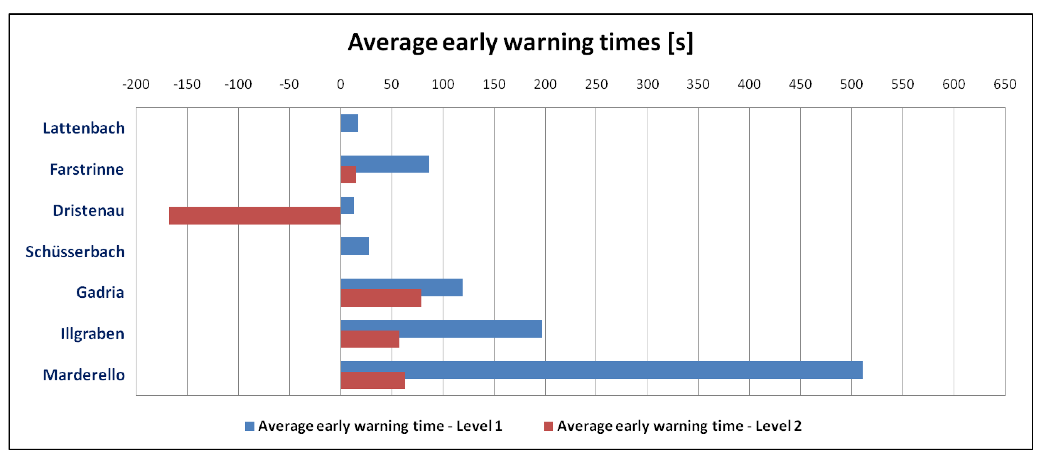
| Average Early Warning Time Level 1 (s) | Average Early Warning Time Level 2 (s) | Number of Events | |
|---|---|---|---|
| Lattenbach | 17 | 1 | 5 |
| Farstrinne | 87 | 15 | 2 |
| Dristenau | 13 | −168 | 4 |
| Schüsserbach | 28 | 0 | 2 |
| Gadria | 120 | 79 | 3 |
| Illgraben | 197 | 57 | 8 |
| Marderello | 511 | 63 | 2 |
| Test Site | Event Date | Peak Discharge (m/s) | Total Volume (m) |
|---|---|---|---|
| Lattenbach | 9 August 2015 | 50 | 11,500 |
| 10 August 2015 | 69 | 18,500 | |
| 16 August 2015 | 12 | 5000 | |
| 10 September 2016 | 158 | 46,000 | |
| Gadria | 15 July 2014 | na | 10,500 |
| 8 June 2015 | na | 9850 | |
| 12 July 2016 | na | 1500 | |
| Illgraben | 22 July 2015 | 17 | 8700 |
| 10 August 2015 | 7 | 6100 | |
| 14 August 2015 | 7 | 25,000 | |
| 15 August 2015 | 3 | 2000 | |
| 12 July 2016 | 15 | 10,000 | |
| 12 July 2016 | 65 | 60,000 | |
| 22 July 2016 | 50–90 | >10,000 | |
| 9 August 2016 | 29 | <10,000 |
© 2018 by the authors. Licensee MDPI, Basel, Switzerland. This article is an open access article distributed under the terms and conditions of the Creative Commons Attribution (CC BY) license (http://creativecommons.org/licenses/by/4.0/).
Share and Cite
Schimmel, A.; Hübl, J.; McArdell, B.W.; Walter, F. Automatic Identification of Alpine Mass Movements by a Combination of Seismic and Infrasound Sensors. Sensors 2018, 18, 1658. https://doi.org/10.3390/s18051658
Schimmel A, Hübl J, McArdell BW, Walter F. Automatic Identification of Alpine Mass Movements by a Combination of Seismic and Infrasound Sensors. Sensors. 2018; 18(5):1658. https://doi.org/10.3390/s18051658
Chicago/Turabian StyleSchimmel, Andreas, Johannes Hübl, Brian W. McArdell, and Fabian Walter. 2018. "Automatic Identification of Alpine Mass Movements by a Combination of Seismic and Infrasound Sensors" Sensors 18, no. 5: 1658. https://doi.org/10.3390/s18051658
APA StyleSchimmel, A., Hübl, J., McArdell, B. W., & Walter, F. (2018). Automatic Identification of Alpine Mass Movements by a Combination of Seismic and Infrasound Sensors. Sensors, 18(5), 1658. https://doi.org/10.3390/s18051658