3D-Subspace-Based Auto-Paired Azimuth Angle, Elevation Angle, and Range Estimation for 24G FMCW Radar with an L-Shaped Array


Abstract
:1. Introduction
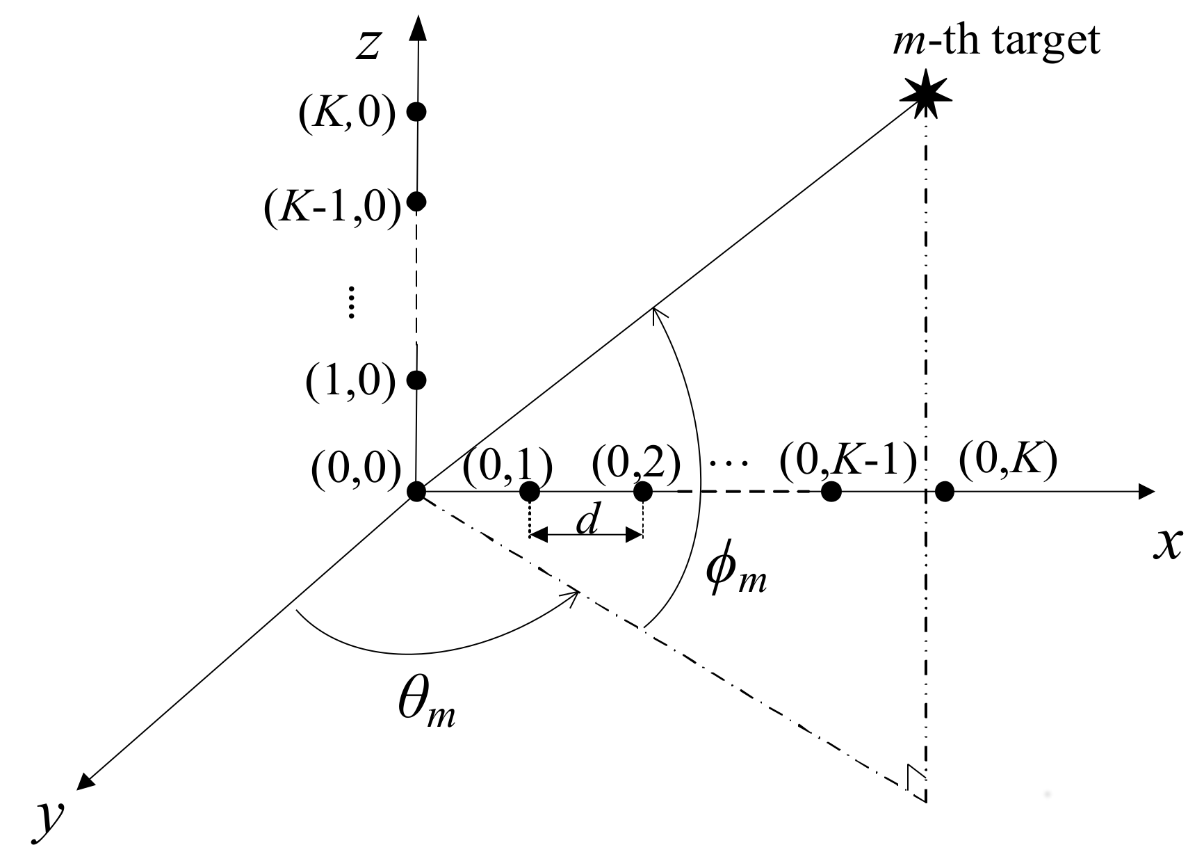
2. System Model
3. Proposed Algorithm
3.1. Shift-Invariant Structure for Range
3.2. Shift-Invariant Structure for Two Electrical Angles
3.3. Signal Subspace
3.4. Low-Complexity Pairing
3.5. Complexity Analysis
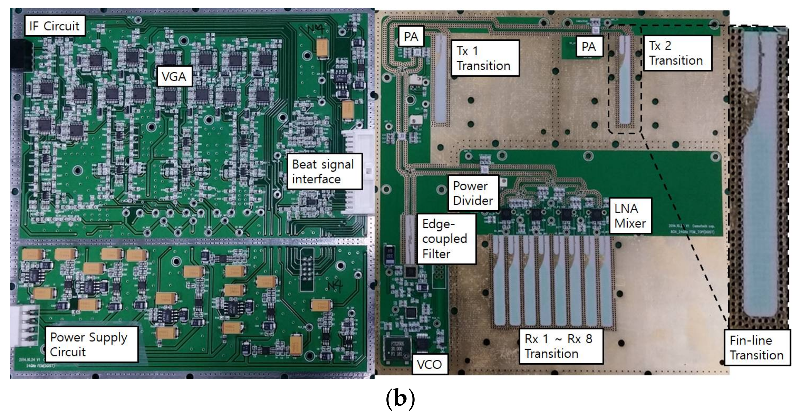
4. Implementation of 24-GHz L-Shaped Radar
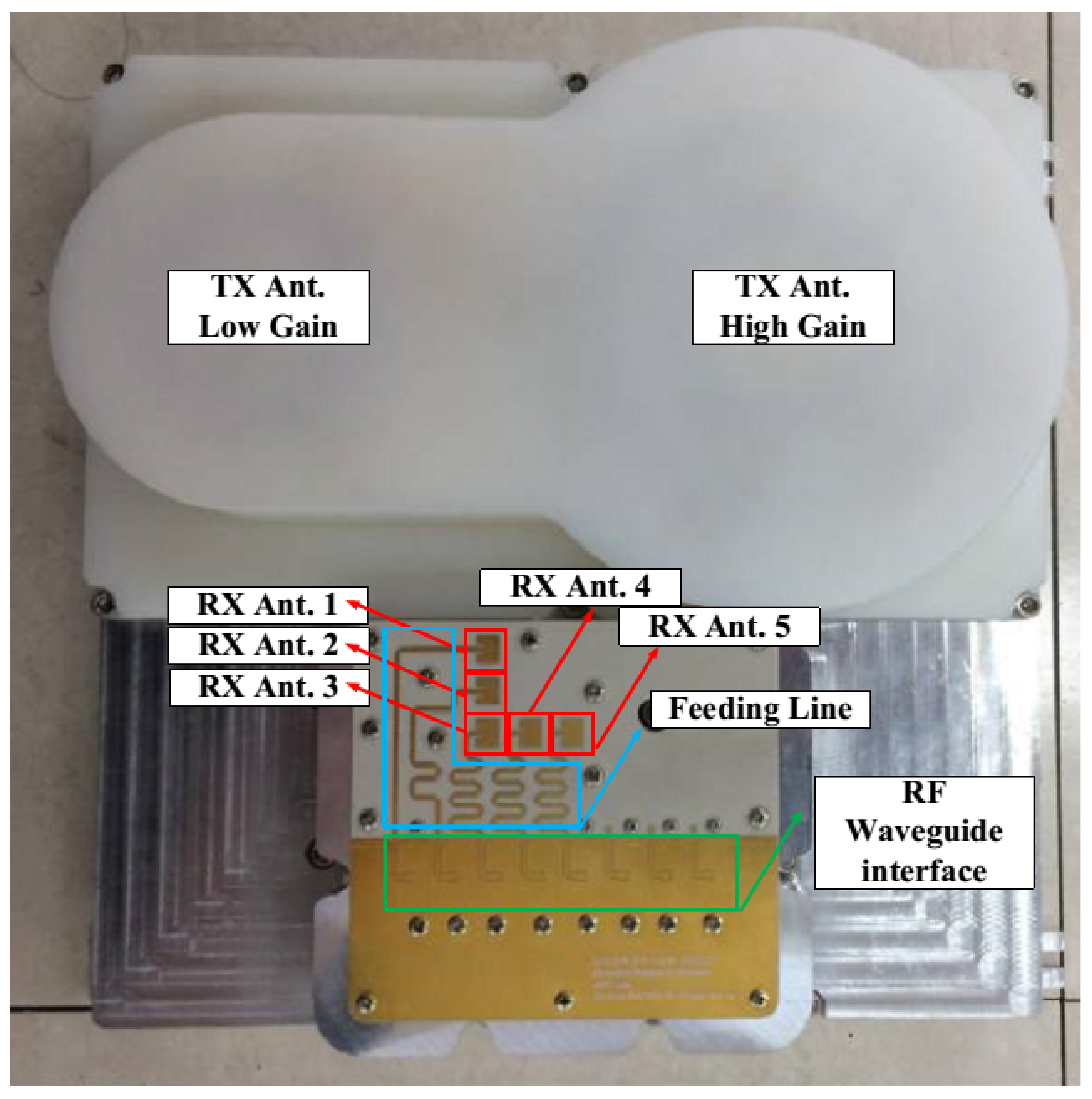
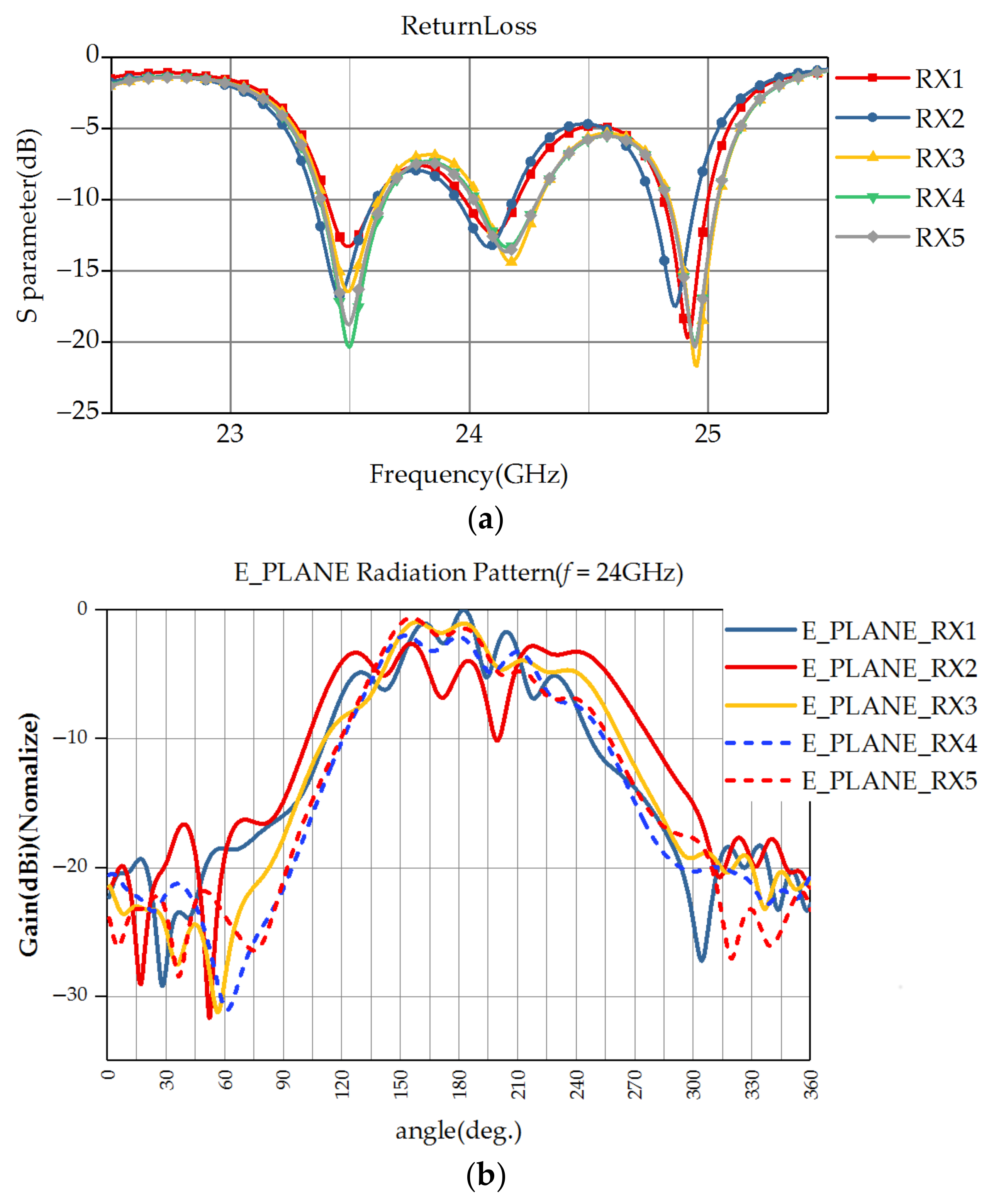
4.1. Transmitting and L-Shaped Receiving Antennas
4.2. 24-GHz Transceiver and IF
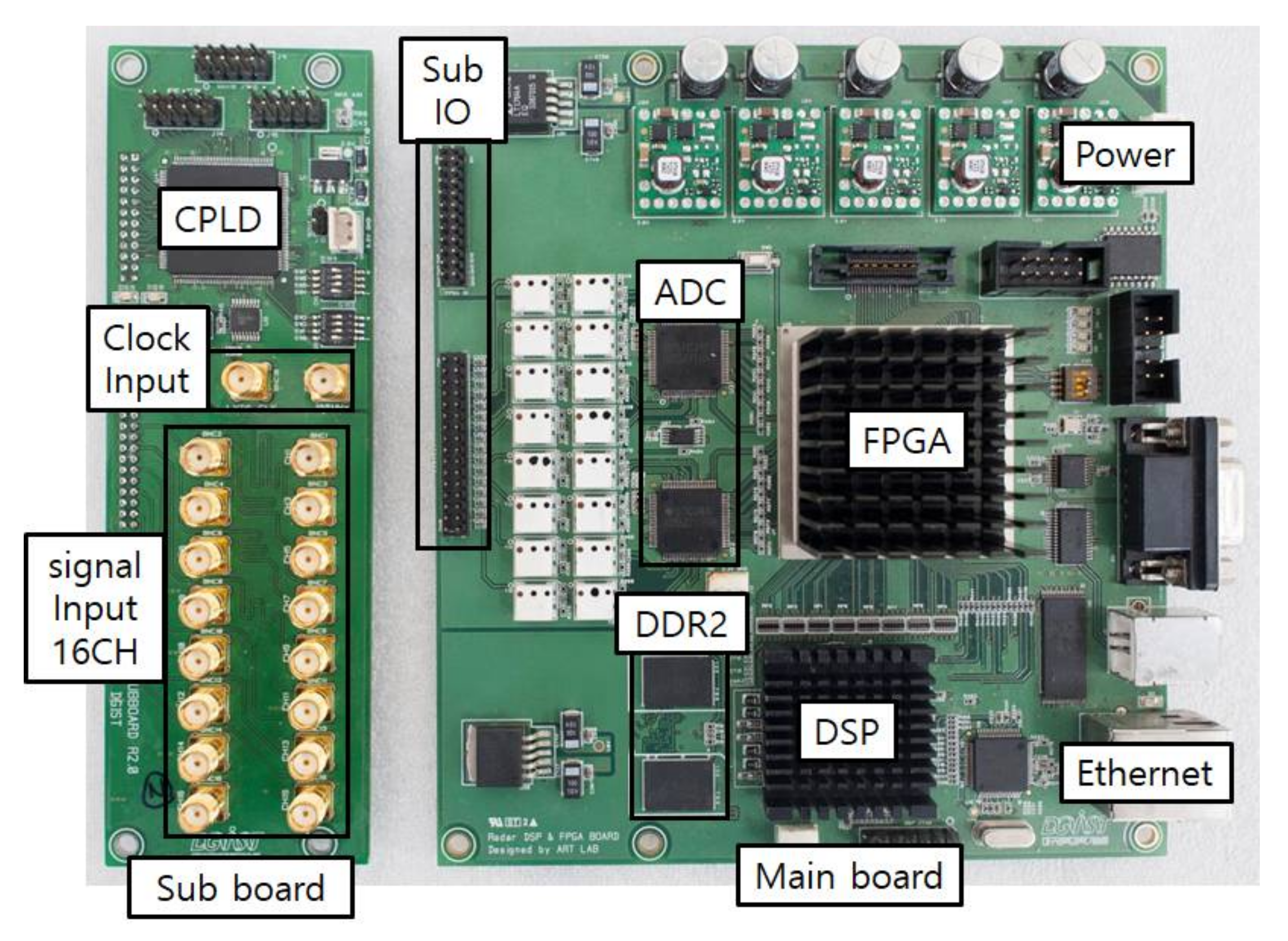
4.3. Data-Logging Platform
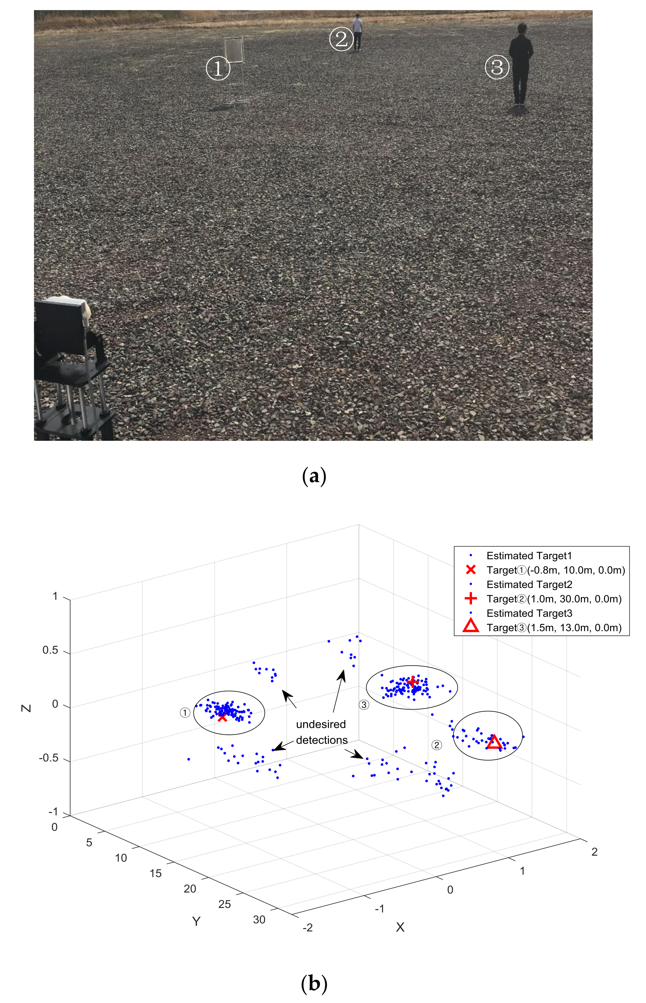
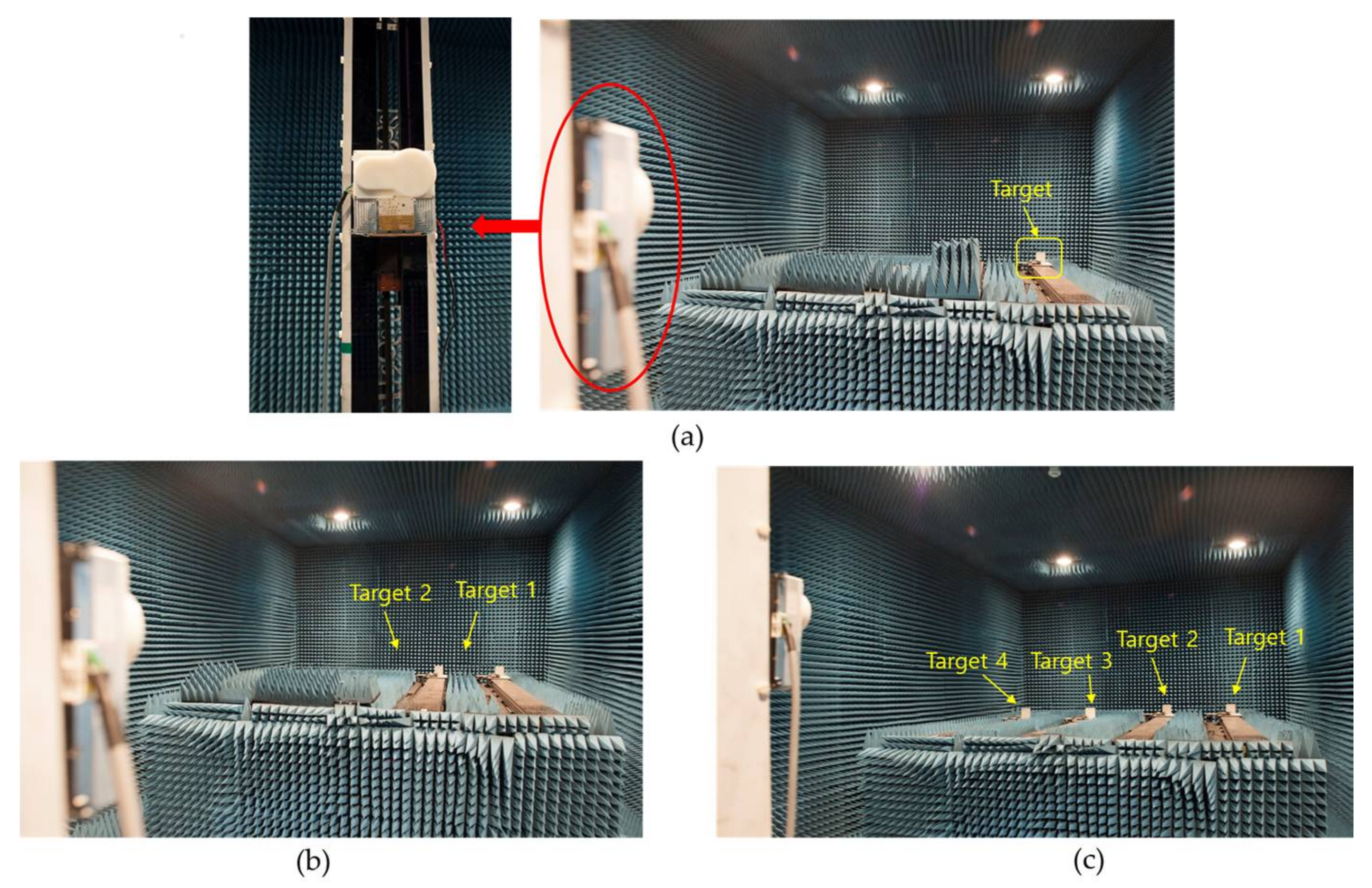
5. Experiments
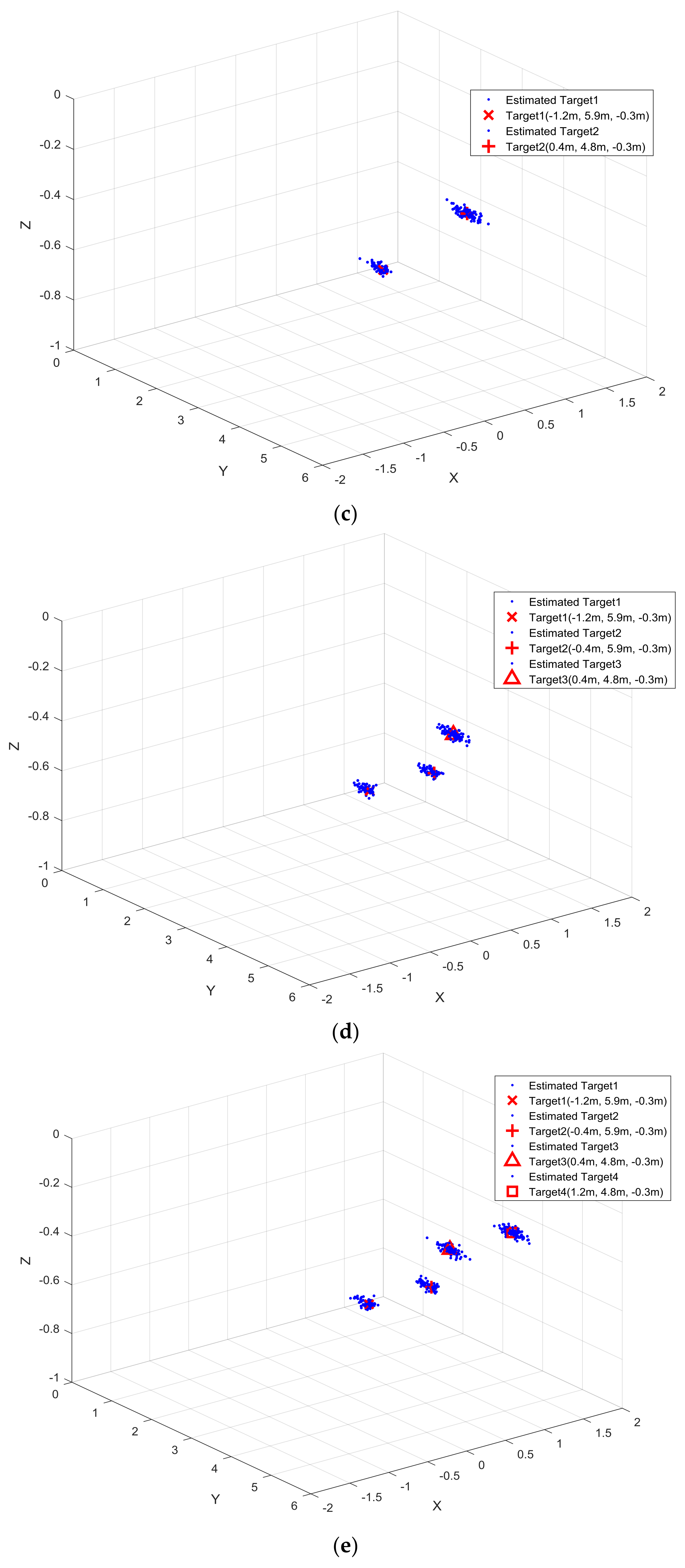
- 1st experiment: one target, Target (−1.2 m, 5.9 m, −0.3 m)
- 2nd experiment: two targets, Target 1 (−1.2 m, 5.9 m, −0.3 m), Target 2 (−0.4 m, 5.9 m, −0.3 m)
- 3rd experiment: two targets, Target 1 (−1.2 m, 5.9 m, −0.3 m), Target 2 (0.4 m, 4.8 m, −0.3 m)
- 4th experiment: three targets, Target 1 (−1.2 m, 5.9 m, −0.3 m), Target 2 (−0.4 m, 5.9 m, −0.3 m), Target 3 (0.4 m, 4.8 m, −0.3 m)
- 5th experiment: four targets, Target 1 (−1.2 m, 5.9 m, −0.3 m), Target 2 (−0.4 m, 5.9 m, −0.3 m), Target 3 (0.4 m, 4.8 m, −0.3 m), Target 4 (1.2 m, 4.8 m, −0.3 m)
6. Conclusions
Acknowledgments
Author Contributions
Conflicts of Interest
References
- Lin, J.-I.; Li, Y.-P.; Hsu, W.-C.; Lee, T.-S. Design of an FMCW Radar Baseband Signal Processing System for Automotive Application. Springer Plus 2016, 5, 42. [Google Scholar] [CrossRef] [PubMed]
- Sevgi, L.; Ponsford, A.; Chan, H.C. An integrated maritime surveillance system based on high-frequency surface wave radars, Part 1. Theoretical background and numerical simulations. IEEE Antennas Propag. Mag. 2001, 43, 28–43. [Google Scholar] [CrossRef]
- Lee, M.S. Signal modeling and analysis of a planar phased-array FMCW radar with antenna switching. IEEE Antennas Wirel. Propag. Lett. 2011, 10, 179–182. [Google Scholar] [CrossRef]
- Ho, T.-J.; Chung, M.-J. Information-aided smart schemes for vehicle flow detection enhancements of traffic microwave radar detectors. Appl. Sci. 2016, 6, 196. [Google Scholar] [CrossRef]
- Kim, I.S.; Jeong, K.; Jeong, J.K. Two novel radar vehicle detectors for the replacement of a conventional loop detector. Microw. J. 2001, 44, 22. [Google Scholar]
- Melzer, A.; Starzer, F.; Jäger, H.; Huemer, M. Real-Time Mitigation of Short-Range Leakage in Automotive FMCW Radar Transceivers. IEEE Trans. Circuits Syst. II Express Briefs 2017, 64, 847–851. [Google Scholar] [CrossRef]
- Peng, Z.; Ran, L.; Li, C. A K-Band Portable FMCW Radar with Beamforming Array for Short-Range Localization and Vital-Doppler Targets Discrimination. IEEE Trans. Microw. Theory Tech. 2017, 65, 3443–3452. [Google Scholar] [CrossRef]
- Cooper, K.B.; Durden, S.L.; Cochrane, C.J.; Monje, R.R.; Dengler, R.J.; Baldi, C. Using FMCW Doppler Radar to Detect Targets up to the Maximum Unambiguous Range. IEEE Geosci. Remote Sens. Lett. 2017, 14, 339–343. [Google Scholar] [CrossRef]
- Liu, J.; Kong, L.; Yang, X.; Liu, Q.H. Refraction Angle Approximation Algorithm for Wall Compensation in TWRI. IEEE Geosci. Remote Sens. Lett. 2016, 13, 943–946. [Google Scholar] [CrossRef]
- Kim, S.; Oh, D.; Lee, J. Joint DFT-ESPRIT Estimation for TOA and DOA in Vehicle FMCW Radars. IEEE Antennas Wirel. Propag. Lett. 2015, 14, 1710–1713. [Google Scholar] [CrossRef]
- Manokhin, G.O.; Erdyneev, Z.T.; Geltser, A.A.; Monastyrev, E.A. MUSIC-based algorithm for range-azimuth FMCW radar data processing without estimating number of targets. In Proceedings of the 2015 IEEE 15th Mediterranean Microwave Symposium (MMS), Lecce, Italy, 30 November–2 December 2015; pp. 1–4. [Google Scholar] [CrossRef]
- Li, J.; Jiang, D. Joint Elevation and Azimuth Angles Estimation for L-Shaped Array. IEEE Antennas Wirel. Propag. Lett. 2017, 16, 453–456. [Google Scholar] [CrossRef]
- Dong, Y.Y.; Dong, C.X.; Zhu, Y.T.; Zhao, G.Q.; Liu, S.Y. Two-dimensional DOA estimation for L-shaped array with nested subarrays without pair matching. IET Signal Process. 2016, 10, 1112–1117. [Google Scholar] [CrossRef]
- Zhang, Z.C.; Shi, Y.W.; Zhang, H. An algorithm for joint angle and frequency estimation in colored noise. In Proceedings of the 2011 International Conference on Uncertainty Reasoning and Knowledge Engineering, Bali, Indonesia, 4–7 August 2011; pp. 219–222. [Google Scholar] [CrossRef]
- Viberg, M.; Stoica, P. A computationally efficient method for joint direction finding and frequency estimation in colored noise. In Proceedings of the Conference Record of Thirty-Second Asilomar Conference on Signals, Systems and Computers (Cat. No.98CH36284), Pacific Grove, CA, USA, 1–4 November 1998; Volume 2, pp. 1547–1551. [Google Scholar] [CrossRef]
- Lemma, A.N.; van der Veen, A.J.; Deprettere, E.F. Analysis of joint angle-frequency estimation using ESPRIT. IEEE Trans. Signal Process. 2003, 51, 1264–1283. [Google Scholar] [CrossRef]
- Li, J.; Wan, G.; Miao, J.; Yang, S. Local Oscillator Phase Noise and its effect on Correlation Millimeter Wave Receiver Performance. In Proceedings of the 7th International Symposium on Antennas, Propagation & EM Theory, Guilin, China, 26–29 October 2006; pp. 1–3. [Google Scholar] [CrossRef]
- Sarkar, T.K.; Pereira, O. Using the matrix pencil method to estimate the parameters of a sum of complex exponentials. IEEE Antennas Propag. Mag. 1995, 37, 48–55. [Google Scholar] [CrossRef]
- Zhang, Y.; Ye, Z. Efficient method of DOA estimation for uncorrelated and coherent signals. IEEE Antennas Wirel. Propag. Lett. 2008, 7, 799–802. [Google Scholar] [CrossRef]
- Wax, M.; Kailath, T. Detection of signals by information theoretic criteria. IEEE Trans. Acoust. Speech Signal Process. 1985, 33, 387–392. [Google Scholar] [CrossRef]
- Oh, D.; Lee, J.H. Low-complexity range-azimuth FMCW radar sensor using joint angle and delay estimation without SVD and EVD. IEEE Sens. J. 2015, 15, 4799–4811. [Google Scholar] [CrossRef]
- Van der Veen, A.J.; Vanderveen, M.C.; Paulraj, A. Joint angle and delay estimation using shift-invariance techniques. IEEE Trans. Signal Process. 1998, 46, 405–418. [Google Scholar] [CrossRef]
- Vanderveen, M.C.; Papadias, C.B.; Paulraj, A. Joint angle and delay estimation (JADE) for multipath signals arriving at an antenna array. IEEE Commun. Lett. 1997, 1, 12–14. [Google Scholar] [CrossRef]
- Chen, V.C.; Qian, S. Joint time-frequency transform for radar range-Doppler imaging. IEEE Trans. Aerosp. Electron. Syst. 1998, 34, 486–499. [Google Scholar] [CrossRef]
- Nyqvist, H.E.; Hendeby, G.; Gustafsson, F. On joint range and velocity estimation in detection and ranging sensors. In Proceedings of the 19th International Conference on Information Fusion (FUSION), Heidelberg, Germany, 5–8 July 2016; pp. 1674–1681. [Google Scholar]
- Hou, H.; Sheng, G.; Jiang, X. Localization Algorithm for the PD Source in Substation Based on L-Shaped Antenna Array Signal Processing. IEEE Trans. Power Deliv. 2015, 30, 472–479. [Google Scholar] [CrossRef]
- Yang, L.; Liu, S.; Li, D.; Jiang, Q.; Cao, H. Fast 2D DOA estimation algorithm by an array manifold matching method with paraller linear arrays. Sensors 2016, 16, 1456. [Google Scholar] [CrossRef]
- Dong, Y.Y.; Dong, C.X.; Xu, J.; Zhao, G.Q. Computationally Efficient 2-D DOA Estimation for L-Shaped Array with Automatic Pairing. IEEE Antennas Wirel. Propag. Lett. 2016, 15, 1669–1672. [Google Scholar] [CrossRef]
- Xi, N.; Li, L.P. A Computationally Efficient Subspace Algorithm for 2-D DOA Estimation with L-shaped Array. IEEE Signal Process. Lett. 2014, 21, 971–974. [Google Scholar] [CrossRef]
- Belfiori, F.; Rossum, W.; Hoogeboom, P. 2D-MUSIC technique applied to a coherent FMCW MIMO radar. In Proceedings of the IET International Conference on Radar Systems (Radar 2012), Glasgow, UK, 22–25 October 2012; pp. 1–6. [Google Scholar] [CrossRef]


| Operation Description | Computational Complexity |
|---|---|
| SVD of Y | O(K2Lc + K+) |
| EVD of G, GX, and GY | O(M3) |
| O(2M2(Lc – 1) + M3) | |
| , | O(2M2(K – 1) + M3) |
| Two-dimensional searching | O(b2K2) |
| Specification | Value |
|---|---|
| Center Frequency | 24.125 GHz |
| Frequency Bandwidth (B) | 200 MHz |
| Frequency Period (T) | 100 μs |
| Transmitter Output Power | 20 dBm |
| Receiver Channel | 5 ch |
| Receiver Noise Figure | 10 dB (max) |
| P1dB of LNA | −15 dBm |
| Receiver Dynamic Range | 60 dB |
| Submodules | Parts | Specification |
|---|---|---|
| FPGA | EP4SE530H35C4N | Logic element: 531,200 |
| Total Internal Memory: 27,376 Kbit | ||
| Embedded Multipliers (18 × 18): 1024 | ||
| DSP | TMS320C6455-1GHz | Cycle Time: 1-ns Instruction Cycle Time |
| Internal Memory: 2096K-Byte | ||
| Memory Interface: 64-Bit, Sync, Async | ||
| DDR2 Controller: 32-Bit, 533 HMz BUS | ||
| DDR2 | MT47H128M16RT | 16 Meg × 16 × 8 Banks × 2EA |
| Flash | AT29LV040A-15TC | 4 Megabit |
| PHY | LX971ALE | 10/100 Mb/s Ethernet PHY |
| ADC | ADS5271 | 12 Bit 8 CH ADC × 2EA, 40 MHz |
| LVDS Interface | ||
| RS232 | MAX3221 | RS-232 Line Driver/Receiver |
| FT232RL | USB UART IC | |
| CPLD | 10M08SAE144C8GES | Logic element: 8000 |
| LABs: 500 |
| Experiments | Target 1 | Target 2 | Target 3 | Target 4 |
|---|---|---|---|---|
| 1st experiment | 0.1775 | |||
| 2nd experiment | 0.1726 | 0.1649 | ||
| 3rd experiment | 0.1595 | 0.1705 | ||
| 4th experiment | 0.1676 | 0.1876 | 0.1658 | |
| 5th experiment | 0.1692 | 0.1775 | 0.1673 | 0.1651 |
© 2018 by the authors. Licensee MDPI, Basel, Switzerland. This article is an open access article distributed under the terms and conditions of the Creative Commons Attribution (CC BY) license (http://creativecommons.org/licenses/by/4.0/).
Share and Cite
Nam, H.; Li, Y.-C.; Choi, B.; Oh, D. 3D-Subspace-Based Auto-Paired Azimuth Angle, Elevation Angle, and Range Estimation for 24G FMCW Radar with an L-Shaped Array. Sensors 2018, 18, 1113. https://doi.org/10.3390/s18041113
Nam H, Li Y-C, Choi B, Oh D. 3D-Subspace-Based Auto-Paired Azimuth Angle, Elevation Angle, and Range Estimation for 24G FMCW Radar with an L-Shaped Array. Sensors. 2018; 18(4):1113. https://doi.org/10.3390/s18041113
Chicago/Turabian StyleNam, HyungSoo, Ying-Chun Li, ByungGil Choi, and Daegun Oh. 2018. "3D-Subspace-Based Auto-Paired Azimuth Angle, Elevation Angle, and Range Estimation for 24G FMCW Radar with an L-Shaped Array" Sensors 18, no. 4: 1113. https://doi.org/10.3390/s18041113
APA StyleNam, H., Li, Y.-C., Choi, B., & Oh, D. (2018). 3D-Subspace-Based Auto-Paired Azimuth Angle, Elevation Angle, and Range Estimation for 24G FMCW Radar with an L-Shaped Array. Sensors, 18(4), 1113. https://doi.org/10.3390/s18041113