Sparse Unorganized Point Cloud Based Relative Pose Estimation for Uncooperative Space Target


1
School of Mechanical Engineering and Automation, Beihang University, Beijing 100191, China
2
State Key Laboratory of Virtual Reality Technology and Systems, Beihang University, Beijing 100191, China
3
Beijing Institute of Control Engineering, Beijing 100080, China
*
Author to whom correspondence should be addressed.
Sensors 2018, 18(4), 1009; https://doi.org/10.3390/s18041009
Submission received: 7 February 2018
/
Revised: 24 March 2018
/
Accepted: 25 March 2018
/
Published: 28 March 2018
(This article belongs to the Section Physical Sensors)
Abstract
:This paper proposes an autonomous algorithm to determine the relative pose between the chaser spacecraft and the uncooperative space target, which is essential in advanced space applications, e.g., on-orbit serving missions. The proposed method, named Congruent Tetrahedron Align (CTA) algorithm, uses the very sparse unorganized 3D point cloud acquired by a LIDAR sensor, and does not require any prior pose information. The core of the method is to determine the relative pose by looking for the congruent tetrahedron in scanning point cloud and model point cloud on the basis of its known model. The two-level index hash table is built for speeding up the search speed. In addition, the Iterative Closest Point (ICP) algorithm is used for pose tracking after CTA. In order to evaluate the method in arbitrary initial attitude, a simulated system is presented. Specifically, the performance of the proposed method to provide the initial pose needed for the tracking algorithm is demonstrated, as well as their robustness against noise. Finally, a field experiment is conducted and the results demonstrated the effectiveness of the proposed method.
1. Introduction
On-Orbit Servicing (OOS), including on-orbit assembly, on-orbit maintenance and on-orbit fueling is an important developing technology for future space systems [1,2,3]. Furthermore, the accurate and reliable relative pose determination between chaser and target is one of the key techniques to accomplish the OOS mission successfully.
The relative pose determination research on cooperative targets [4,5,6], which are equipped with a set of artificial active or passive markers on the target surfaces that can be easily detected and recognized in the acquired datasets, has many achievements and some of them [7,8] have been successfully applied in orbit. However, it is more challenging to estimate the relative pose of the uncooperative targets without cooperative information, especially for the fast-moving targets, such as the high-speed tumbling uncooperative target. Therefore, the pose estimate accuracy and the computational cost have put forward higher requirements. According to the different electro-optical (EO) sensors on the chaser, the study of the uncooperative target is generally divided into the relative pose calculation based on passive systems (e.g., monocular and stereo system) and active systems (e.g., LIDAR). In addition, methods of multi-sensor information fusion are proposed [9,10], e.g., monocular and LIDAR. The methods based on the passive system tend to achieve better accuracy, but they are time-consuming and susceptible to illumination changes. However, the LIDAR system has stronger robustness for illumination.
This paper proposes a novel method of relative pose determination using the very sparse unorganized point cloud acquired by the scanning LIDAR sensor. We propose a Congruent Tetrahedron Align (CTA) method to calculate relative pose directly by searching congruent tetrahedron in scanning point cloud and model point cloud which is acquired from the known 3D CAD model of target. Moreover, this method does not need the time consumption process such as extracting feature [11] or calculating the normal which is a line perpendicular to the local surface represented by a point and its neighbors, and that does not need dense point cloud. The Iterative Closest Point (ICP) [12] algorithm which has advantages of high precision and high speed, can be used for pose tracking since the initial pose has been obtained.
The rest of this paper is organized as follows. In Section 2, the related works in recent years are described in detail. In Section 3, the details of proposed pose estimation method are presented. Then, we analyze the influencing factors of the proposed method in Section 4. Experiments and conclusions are shown in Section 5 and Section 6, respectively.
2. Related Work
The research on relative pose determination of uncooperative targets is a fundamental problem for OOS application. Because of their lower hardware complexity, their lower cost and their lower power consumption, passive systems have been widely considered in the research field of relative position calculation of space non-cooperative targets [13,14,15].
Methods based on monocular cameras that rely on various Perspective-n-Point problem (PnP) solvers [16,17,18] have been proposed to calculate the initial relative pose. Lepetit et al. [16] proposed efficient PnP (EPnP) solvers with the main idea of expressing the reference points as a weighted sum of four non-coplanar virtual control points. D’Amico [14] proposed the Newton-Raphson method to solve the PnP iteratively. Due to its use of least squares, which is very suitable for handling Gaussian noise, it has a high accuracy even in the presence of outliers or noise. In addition, the two-dimensional Template Matching (2D TM) approaches [19] are usually advanced in high accuracy and good anti-noise performance. Cai et al. [15] proposed a hollow annulus structure according to the Features from Accelerated Segment (FAST) feature to match the template and object image by comparing the differences of both grey and gradient. It is very important and challenging to obtain the correct correspondence between the features extracted from the image and the target model before approaching the PnP solvers. Besides the method based on point features, some others used the line features, which are typically more stable than points. For the stereo system, SoftPOSIT [20] that combines the iterative soft-assign algorithm [21,22] and the iterative POSIT algorithm [23] has achieved good accuracy. However, all the above methods generally take more than one second. Hence, when there are other celestial bodies in the field of view, it is not easy for the passive system to distinguish correctly, and the performance is obviously affected by the spatial illumination. In contrast, the active system of LIDAR system has the stronger robustness to the space illumination, and is easier to differentiate targets from the background. Therefore, the methods based on LIDAR are receiving more and more extensive research.
3D TM algorithm [24,25] evolves from the 2D TM algorithm we introduced above. In the process of 3D TM algorithm, a pose space database is generated from a set of views of the 3D target model. Then, the best initial pose estimate is defined as the pose that produces the best correlation with the measurement data. In order to get sufficient accuracy, this method needs to search the entire pose space, which also leads to high computational cost and limits its real-time spatial application. Hence, Opromolla et al., adopt an on-line 3D TM algorithm [26,27,28] to overcome this limitation. Specifically, the relative position is computed by the centroiding approach, thus, the amount of templates is reduced, and the database of templates can be cut down to 3-DOF. In order to further reduce the calculation time, the Principal Component Analysis (PCA) method is used to estimate the main axis, and the database is cut down to 1-DOF, which significantly reduces the searching time. However, the target is required to have an elongated shape.
Besides that, there are some feature-based methods. John O. Woods and John A. Christian proposed an Oriented, Unique, and Repeatable Clustered Viewpoint Feature Histograms (OUR-CVFH) algorithm [11,29], which has the same runtime complexity as ICP (in many cases it runs more quickly), provides free object recognition, and is robust to many types of occlusion. Specifically, a database consists of a set of 303-bin OUR-CVFH histograms describing that each segmented object is built off-line. The OUR-CVFH works when the LIDAR data are obtained with multiplicative EKF to provide a propagated pose estimate before refining the estimate using ICP. This feature-based method generally requires evenly distributed high resolution 3D data to calculate the normal of points.
In addition to the 3D TM methods and feature-based methods described above, the original point-based approaches have also been proposed for space applications. Liu et al. proposed a novel global point cloud registration algorithm based on the translation domain estimation method [30]. The translation domain is estimated by calculating the relative displacements of the axis-aligned bounding box (AABB) in the three main directions of the model point cloud and the scanning point cloud. Then, the GO-ICP algorithm [31], combined BnB (Branch-and-Bound) strategy [32] and ICP algorithm is used to search the optimal estimate. The Polygonal Aspect Hashing (PAH) algorithm [33] proposed by Ruel et al., provides 6-DOF relative pose information in real time based on the idea of puzzles, which aligns the model surface to one or more polygons extracted from scanning point cloud data.
The paper presents another point based method called CTA for the acquisition of the initial pose improved from PAH. The CTA algorithm finds the congruent tetrahedrons, which are from model point cloud and scan point cloud respectively. Some other algorithms for CTA are combined in the process. Specifically, 3D hull algorithm is used to construct a 3D convex from scanning point cloud data for selecting a tetrahedron, and a two-level index hash table is used to speed up the congruent tetrahedron searching speed.
3. Proposed Relative Pose Determination Method
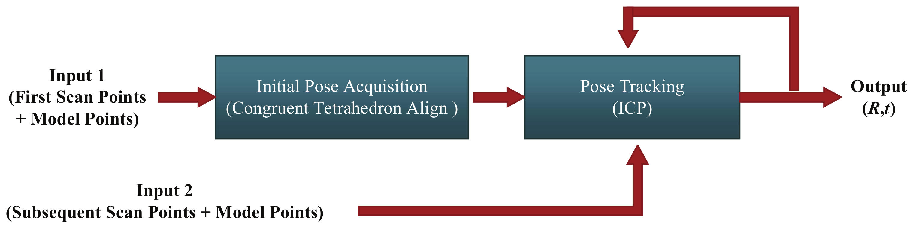
The logical scheme of the process to determine relative pose of uncooperative target is shown in Figure 1. The process is divided into two main steps, named initial pose acquisition and pose tracking, respectively. The proposed CTA algorithm is applied in the initial pose acquisition process when the first scan point cloud is obtained from the scanning LIDAR. The model point cloud can be obtained from the 3D CAD model, which is known. Pose tracking is performed by means of ICP algorithm, which requires a good initial pose estimate. The details of the proposed method are described in the following parts of this section.
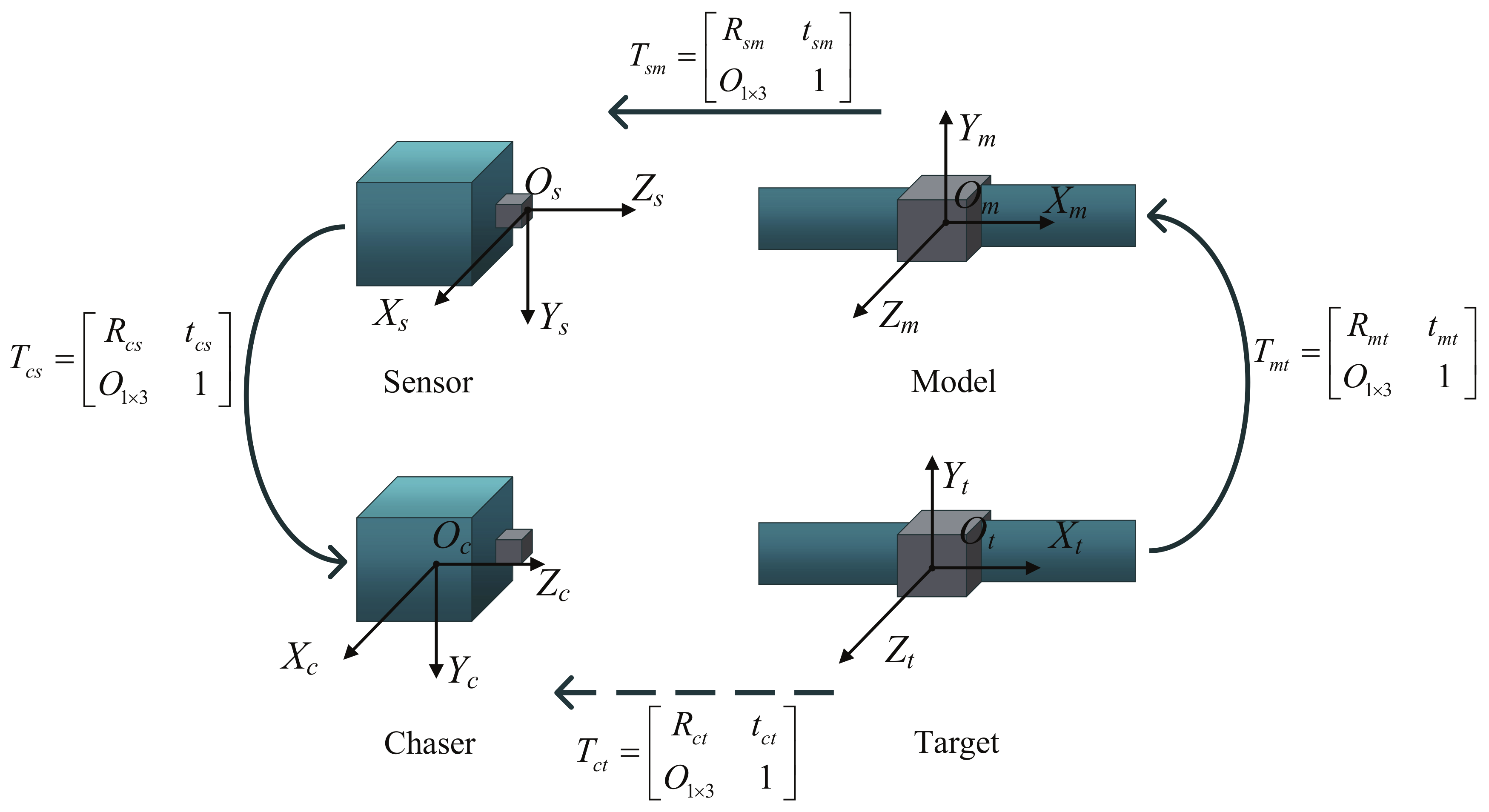
Relative pose determination is the problem of calculating the 3D rotation and translation between chaser and target (Figure 2). Furthermore, four reference frames are of interest: the chaser body-fixed frame OXYZ, the sensor frame OXYZ, the target model frame OXYZ, and the target body-fixed frame OXYZ.
denotes the transformation (including rotation and translation) from frame j to frame i. Generally, can be measured offline, depending on the assembly relation of chaser and sensor. can be obtained from the definition of model frame. , the rotation and translation from target to chaser, can be calculated by Equation (1), where due to the achievable knowledge of and , we only need to calculate .
3.1. CTA Algorithm
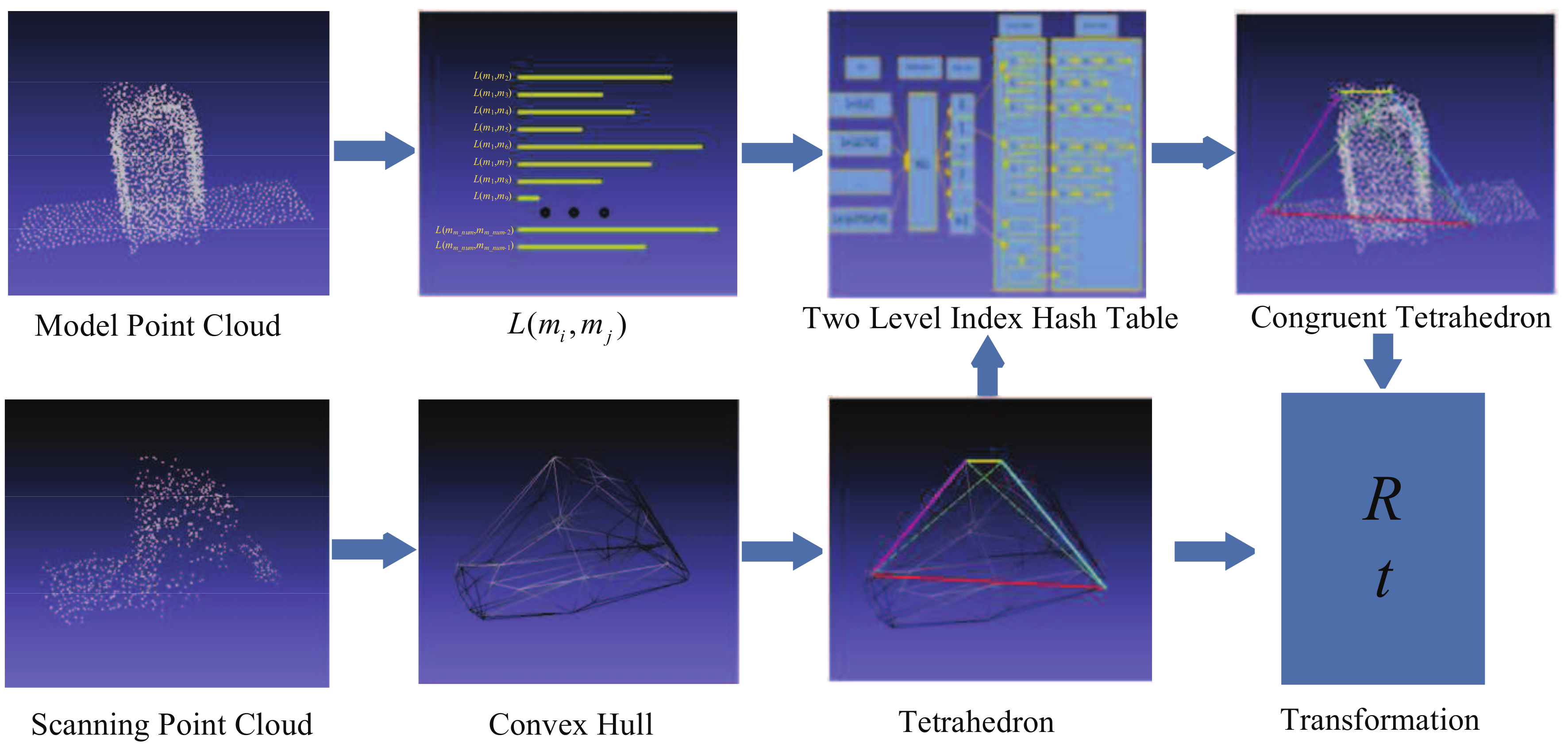
Essentially, the relative pose determination, or registration, consists of finding the overlap between the model point cloud and the scan point cloud, and then calculating the relative transformation. Instead of extracting features, our method finds the congruent tetrahedron directly from the scanning point cloud and model point cloud, and then estimates the relative pose by aligning the congruent tetrahedron. The procedure of the algorithm is illustrated in Figure 3. The model point cloud is sampled from the known 3D CAD model of target. Let be the length of point pairs in the model point cloud. In order to search the corresponding point quickly and accurately, a two-level index hash table which has a low-time complexity of looking up is designed for storing the point pair length as well as the location topology information. When the scanning point cloud is obtained, a 3D convex hull will be constructed to simplify it. Then a tetrahedron with the largest volume is found in the vertices of the convex hull. According to the congruence theorem for tetrahedra, the corresponding tetrahedron of is found in the model point cloud, and then the transformation between them will be calculated.
3.1.1. Congruent Tetrahedron Searching Based on Two-Level Index Hash Table
One of the necessary and sufficient conditions for two tetrahedrons to be congruent is as follows: If six sides of a tetrahedron are equal to the corresponding six sides of another tetrahedron, then the tetrahedrons are regarded as being congruent. Therefore, we find the congruent tetrahedrons, which are respectively from model point cloud and scanning point cloud according to the equal corresponding six sides. In order to find the corresponding sides conveniently and rapidly, we use the two-level index hash table to store the information, which includes not only the point pair length of model point cloud but also the location topology information as will be shown in section A. And in section B, the process of finding the corresponding tetrahedron will be introduced.
A. Building the two-level index hash table
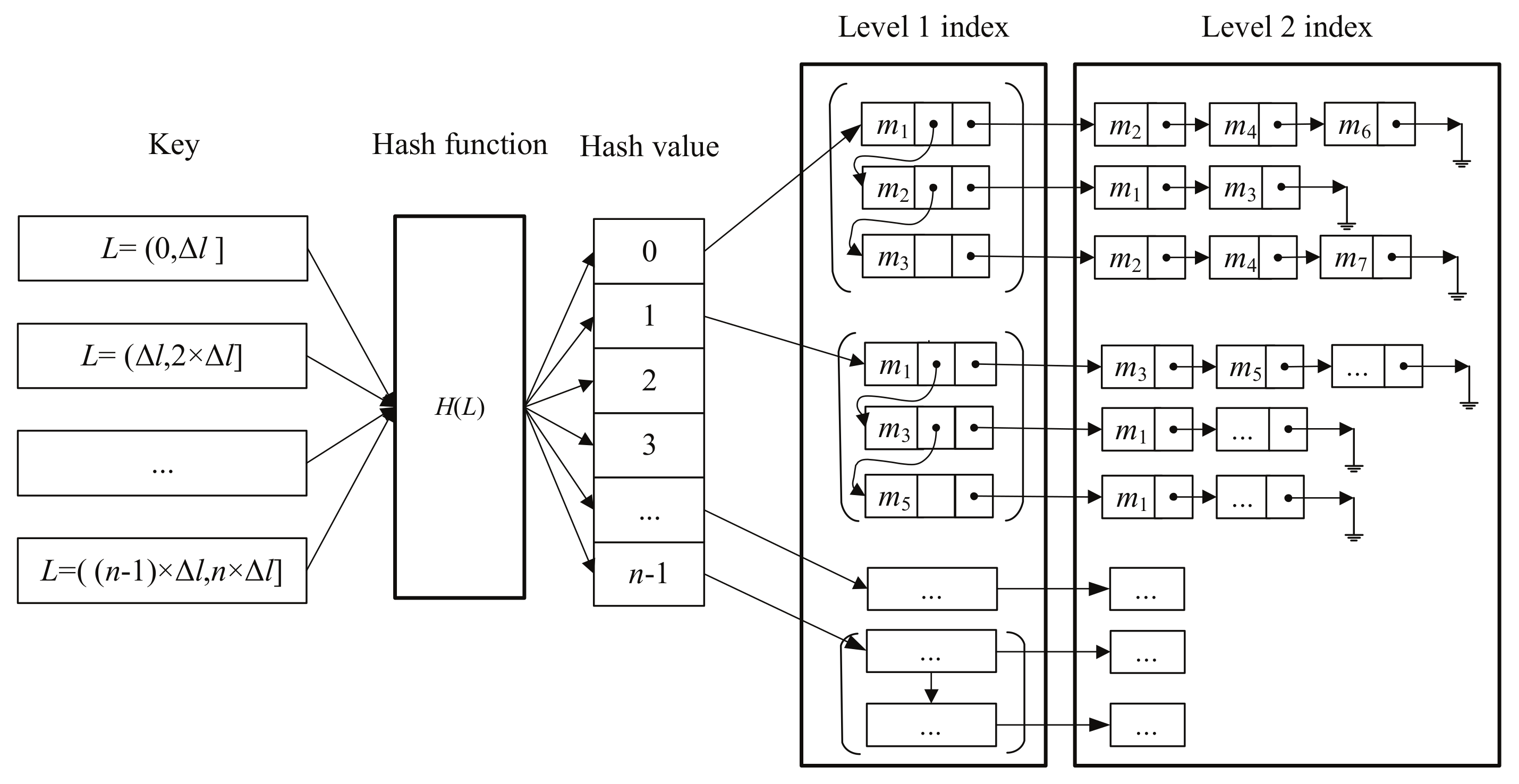
Since the principle of finding two congruent tetrahedrons is to find corresponding sides with equal length, we use a linear hash function to hash the model point cloud into the corresponding buckets, as given in Equation (2).
where, L is the Euclidean distance of model point pair , , , , , N is the number of model points. , is the maximum Euclidean distance between two points of model point cloud. , is the minimum Euclidean distance between two points of model point cloud. is the number of buckets. k is the hash value, .
With the Equation (2), all the point pairs, with the distance in the interval are stored in the bucket. In the bucket, the first element and the second element of point pairs are stored in level 1 index, and level 2 index, respectively. The process of building the hash table is shown in Figure 4.
B. Searching the congruent tetrahedron
Assuming is the tetrahedron founded in scanning point cloud with vertexes , , , . is the two-level index hash table built with model points. The process of searching the congruent tetrahedron with vertexes , , , in hash table is shown in Algorithm 1.
| Algorithm 1 Searching the congruent tetrahedron |
| Input: : four vertexes of ; : hash table |
| Output: : four vertexes of |
|
3.1.2. Selection Tetrahedron from Scanning Point Cloud
The farthest pair of points are extreme points on convex hull. Intuitively, the larger the volume of the tetrahedron is, the stronger the resolution is. Therefore, the selection of tetrahedron is carried out according to the principle of maximum volume. The vertexes of the tetrahedron with the largest volume must be the vertexes of the convex hull. Hence, the convex hull of scan point cloud is first constructed.
3.1.3. Calculation of Transformation
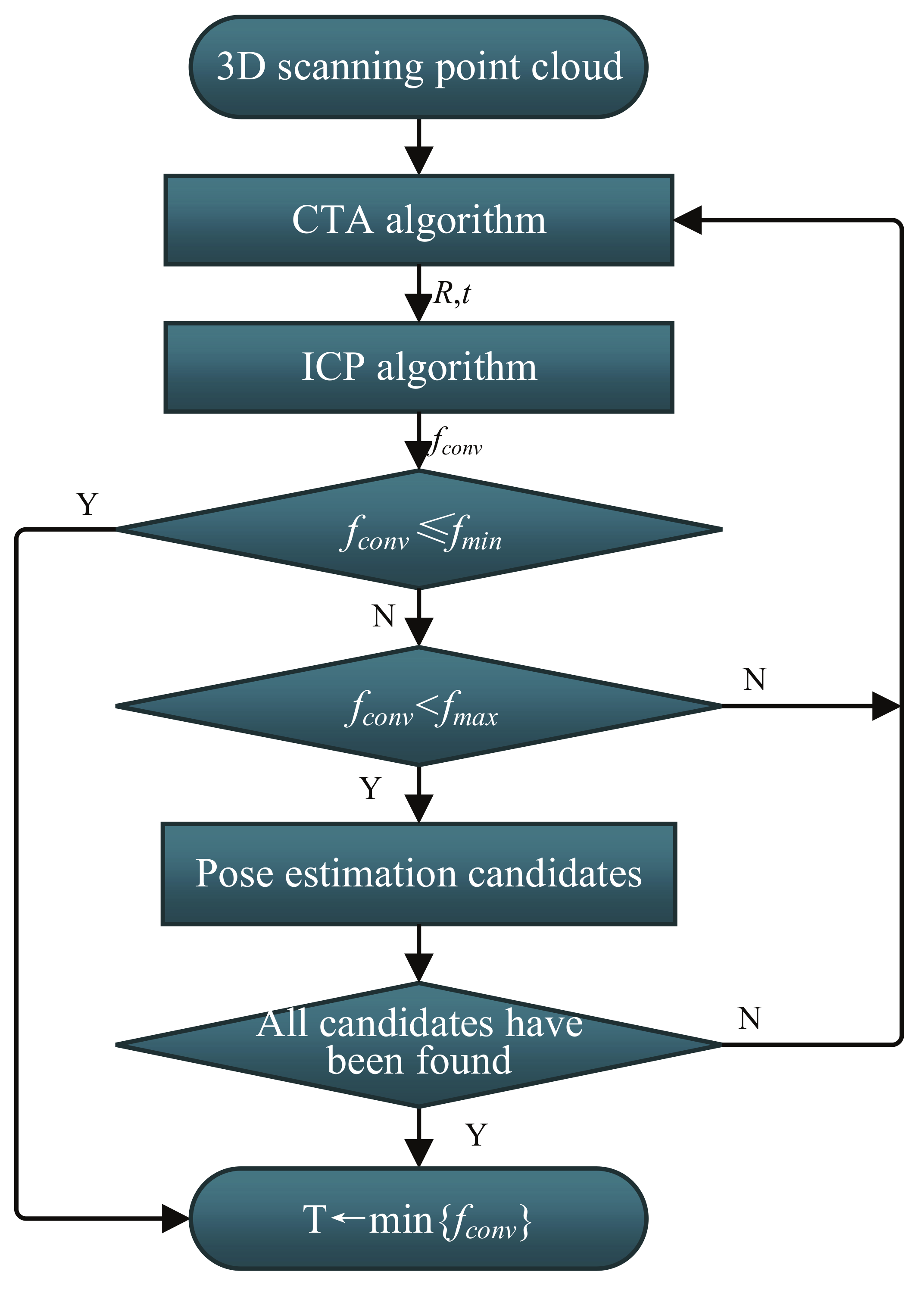
3.1.4. CTA Failure Detection Approach
In general, more than one corresponding tetrahedron can be found in the hash table, but only one is correct. In order to deal with this case and choose the correct one, a strategy is used to detect the failure of the CTA algorithm autonomously. The logic of the approach is shown in Figure 5. When a corresponding tetrahedron is found, the relative transformation is calculated as described in Section 3.1.3 and the transformation is applied to the whole scanning point cloud. After that, the ICP algorithm is used to refine the registration result. The accuracy measurement of the algorithm is ICP convergence score , the value of the closest point to the Euclidean distance which is calculated by Equation (5). Moreover, two threshold values and are set up. If , the registration is believed to be correct, then it is used as the input parameters of the pose tracking stage. Otherwise, if & , it is saved as a candidate, until all of the candidates are looked up in the hash table. After that, choose the transformation corresponding to the smallest as the output of the CTA for the input of the pose tracking.
3.2. Pose Tracking
The output of CTA will be used as the input of pose tracking and the ICP algorithm is used for pose tracking. Although the CTA algorithm has a high success rate, which has been verified in Section 5, a stability strategy is added in order to further guarantee the correctness of the initial pose. The strategy is shown as follows:
- (1)
- For the first scanning point cloud, using CTA algorithm to calculate the transformation ;
- (2)
- For the second frame, using CTA algorithm to calculate the transformation ;
- (3)
- For the second frame, calculating the transformation using as the initial pose in another thread;
- (4)
- Computing the relative translation between and , , and the Euler angles , , can be determined from . If ( are the thresholds), the CTA algorithm is considered as a stable and accurate initial value, and then goto step (5). Otherwise, the result of the CTA algorithm is incorrect, then replace with and go to step (3);
- (5)
- For the subsequent frames, using ICP algorithm to calculate the transformation for pose tracking.
4. Analysis of Influence Factors
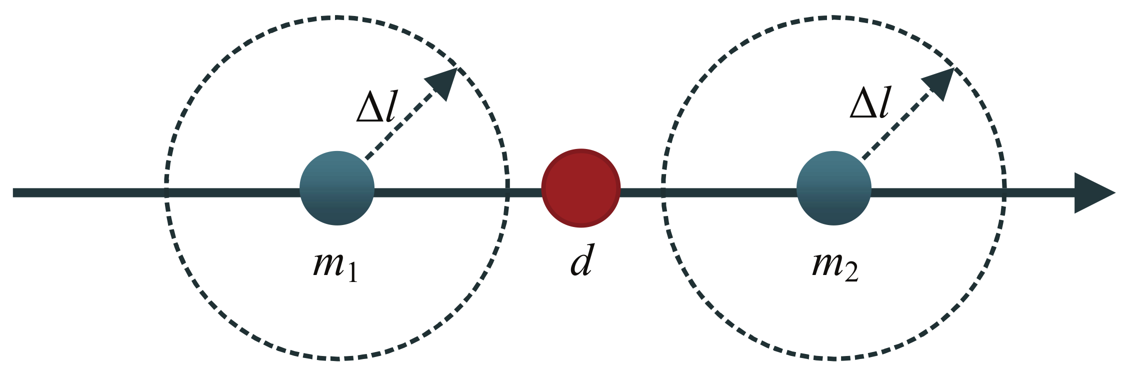
According to hash function (Equation (2)) and the process of searching in the hash table, the main influencing factors are the number of buckets which is equivalent to , and the number of point pairs in each bucket which is related to the distance interval of the model point cloud . As shown in Figure 6, and are points of model point cloud, d is one of the ideal corresponding points in , and are adjacent to d. If , then it could not guarantee that d will fall into the bucket that contains or/and . This means that it may not be possible to find the correct match in the hash table. Only when , it can be ensured that no matter how the distance grid around d is divided, d must be in the bucket that contains or/and .
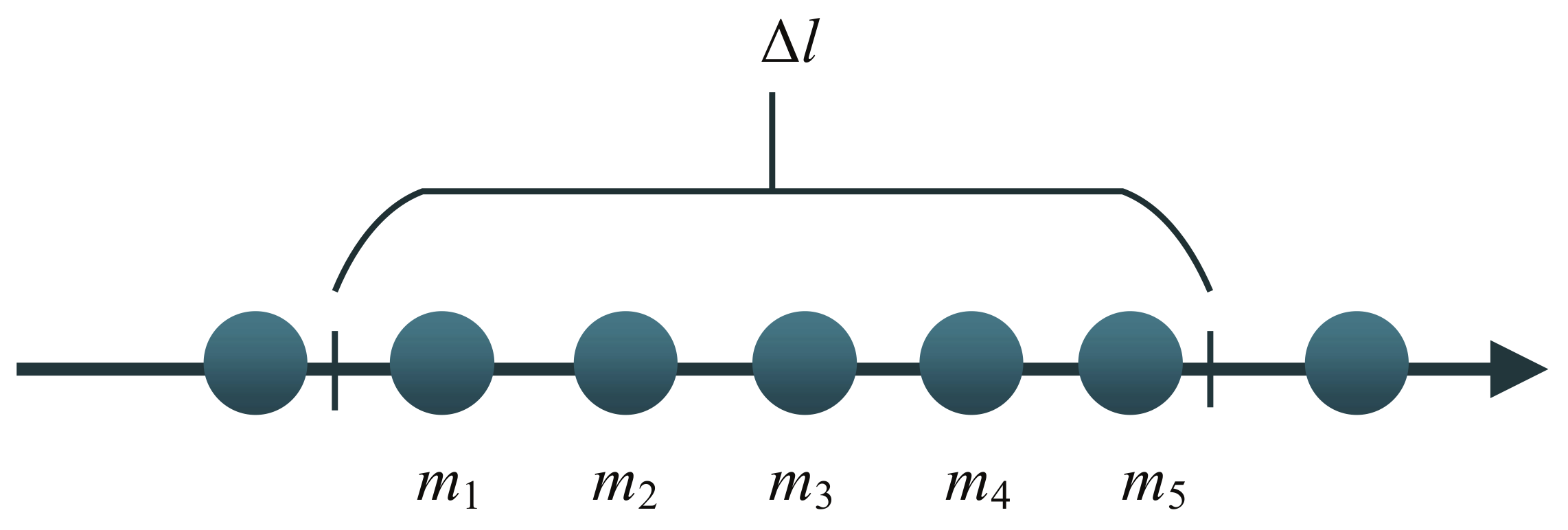
Taking account of all the point pairs of model points, it can be ensured that the match candidates contain the global optimal matching, as long as ( is the largest distance interval of the model point cloud). However, if is much larger than the other interval, more points will be hashed in the same bucket as shown in Figure 7. Assuming that is the correct model point corresponding to s, a vertex of . All of the sides containing will be retrieved as equally as possible to replace with ,, and . Therefore, it is easy to bring redundant matches to increase . Simply, if ( is the smallest distance interval of the model point cloud), we can get a balance between time and accuracy. Therefore, the model point cloud be sampled uniformly at a interval of , and let .
5. Experiments
In this section, we have performed numerical simulation experiments and a field experiment to test the performance of the algorithm. In the experiments, the target is a 1:6 scale satellite model as shown in Figure 8. The size of scale target model is . Simulations are carried out in C++ environment run by a commercial desktop PC equipped with an Intel I5 CPU at .
5.1. Simulation System
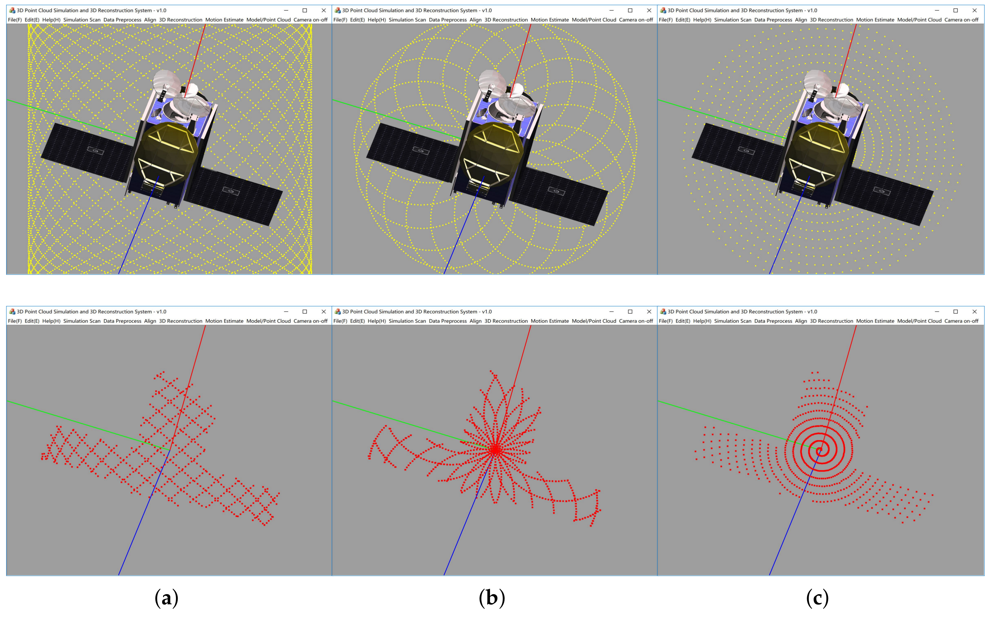
We also developed a 3D point cloud simulation software. After entering the 3D model, and set the relevant scanning parameters, the output of the laser scanner can be simulated. 3D point cloud simulation software is as shown in Figure 8:
In the simulation system, the three scanning patterns of Lissajous, Rosette and Spiral, all of which can cover an area in the fastest time [38], are implemented. The Rosette and Spiral patterns have a high density of points in the middle of the field of view, which will increase the number of points and lead to a more time-consuming process of constructing the 3D convex hull. By contrast, the Lissajous pattern can obtain more uniform points in the middle of the field of view. Therefore, the Lissajous pattern is better in filed experiments. In order to ensure the consistency of the simulation and field experiments, all experiments were conducted using the Lissajous pattern.
5.2. Impact of Different
According to the discussion in Section 4, the point cloud of model should be uniform. We use the software of Geomagic Studio to convert the 3D geometric model to point cloud, and further reduce the number of points uniformly to 484 with the interval = (348 mm∼521 mm). The two parameters and involved in the algorithm are interrelated through the analysis. The impact of on the CTA algorithm and the relative between and are verified in the case of fixed obtained above.
Through Equation (2), and are equivalent. Therefore, in this section we discuss the efficiency of different on the accuracy and speed of the algorithm. After the equidistant sampling of the model point cloud, the interval is about (348 mm∼521 mm). During the process of acquiring the simulated scanning point cloud, the noise with standard deviation of 200 mm is added in the direction of the ray. The average estimation pose errors of different are shown in Table 1. All of the Euler angles in the experiments use the Z-X-Y convention.
According to Equation (2), = 28∼19 under the = (348 mm∼521 mm). From the results in Table 1, it is obvious that with the increase of the number of buckets, the registration time gradually decreases and the registration error rate increases. When the is between 20 and 30, better registration accuracy and lower error rate are achieved, and the registration time is less than 100 ms. This conclusion is consistent with the discussion in Section 4.
In order to balance the registration time and the registration accuracy, is taken in the following experiments.
5.3. CTA Algorithm Test
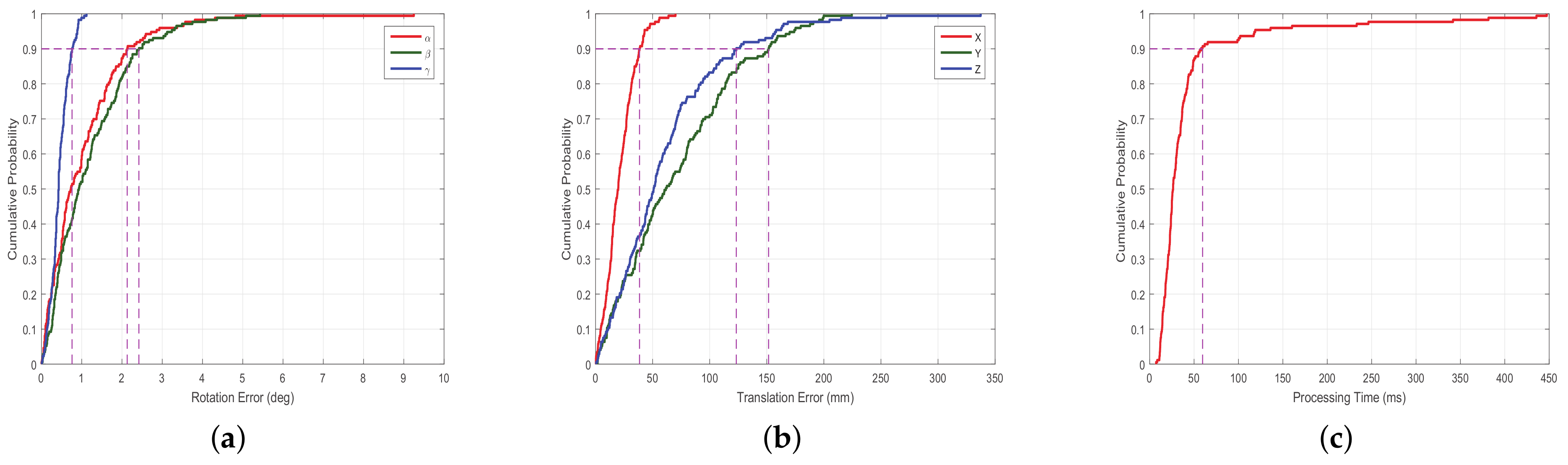
The accuracy of pose tracking is closely related to the initial attitude estimation results, so it is necessary to test the performance of initial attitude estimation algorithm CTA. In this simulation experiment, we also added the noise with standard deviation of 200 mm in the direction of ray and selected 10 groups of 20 positions for testing. The absolute error of initial translation error, initial rotation error and time consuming are given in Figure 9.
Figure 9 shows the Cumulative Distribution Function (CDF), we can see that the proposed relative pose estimation method can estimate the real-time relative pose effectively. The 90% translation error is less than 150 mm, and 90% rotation error is less than . Furthermore, we can see that 90% time-consuming is less than 70 ms. The time-consuming and accuracy of transformation satisfy pose tracking.
5.4. Pose Tracking Test
To test the efficiency of the proposed method for pose tracking, simulated experiments for tumbling targets, which exist widely in space, are carried out under the following different conditions.
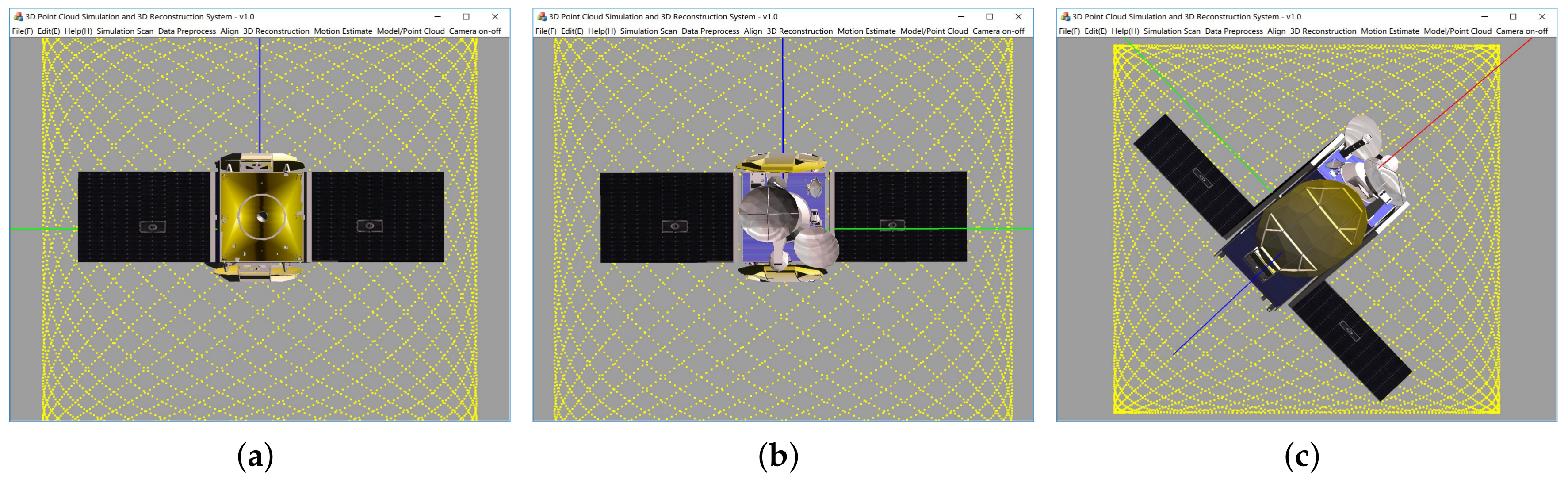
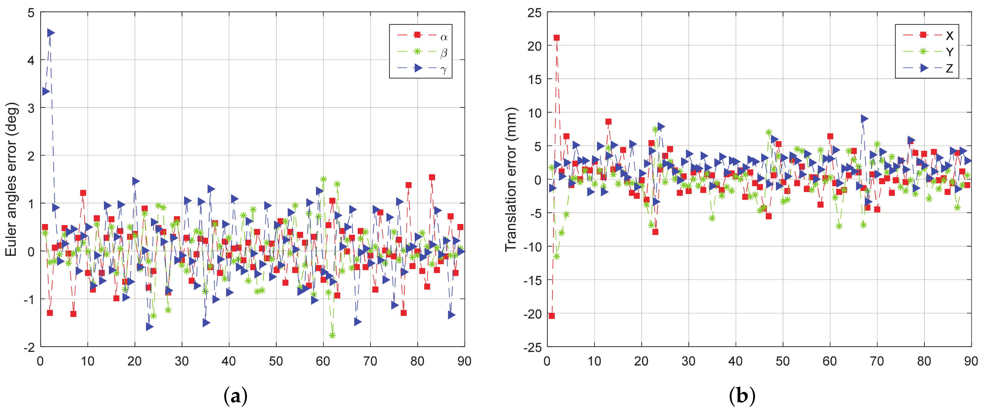
In test 1, the initial attitude is set to , as shown in Figure 10a, and the target rotates around the model’s Y-axis (blue axis). For each simulated point cloud, the is changing from to at interval;
In test 2, the initial attitude is set to , as shown in Figure 10a, and the target rotates around the model’s Z-axis (axis perpendicular to the solar array of the model and perpendicular to the screen). For each simulated point cloud, the is changing from to at interval;
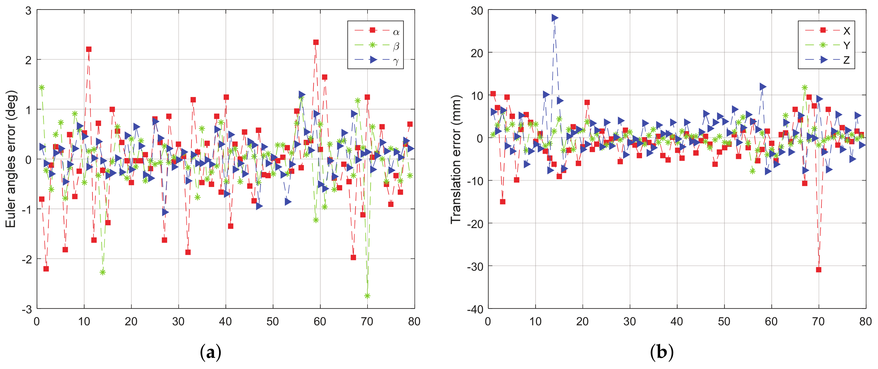
In test 3, the initial attitude is set to , as shown in Figure 10b, and the target rotates around the model’s Z-axis (axis perpendicular to the solar array of the model and perpendicular to the screen). For each simulated point cloud, the is changing from to at interval;
In test 4, the initial attitude is set to , as shown in Figure 10c, and the target rotates around the model’s Z-axis (axis perpendicular to the solar array of the model).
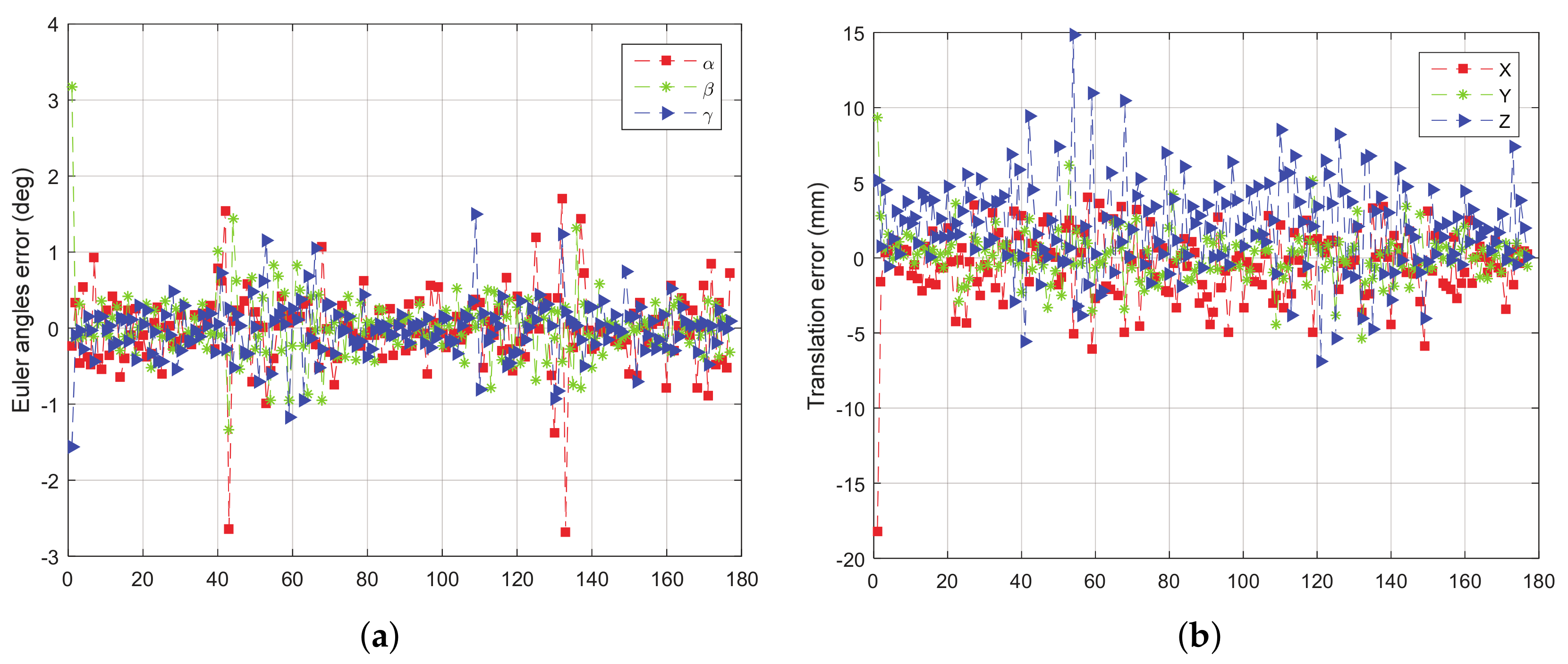
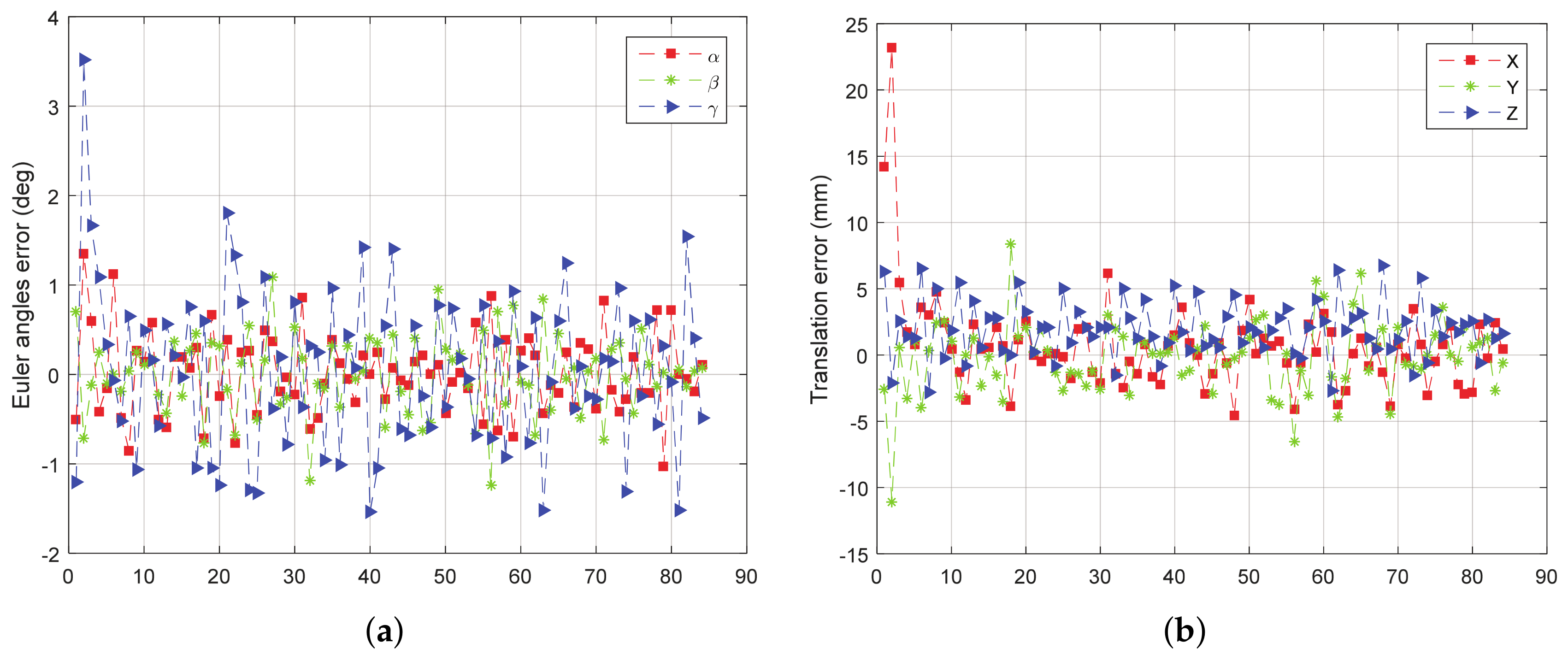
When simulating the LIDAR to get point cloud, the white noise with a standard deviation of is added in the direction of the simulated rays. The rotation error and translation error of the four tests are given from Figure 11, Figure 12, Figure 13 and Figure 14.
From Figure 11, Figure 12, Figure 13 and Figure 14, we can see that, the rotation error is almost less than , and the translation error is almost less than 10 mm in different initial attitudes and different rotation axes. This indicates that the CTA computing initial position proposed in this paper, and pose tracking by ICP algorithm is accurate, fast and robust. However, there also exist some outliers which can be divided into two groups. One of the groups appears in the first few frames, which is due to the large error of the initial pose estimation. The other group appears in the frames, e.g., frame 43 and 133 in Figure 11a, in which the LIDAR can only scan a small part of the target. Under this condition, the feature of the scanning point cloud is not obvious. At the same time, the standard ICP algorithm tends to fall into a local optimal solution, leading to an increase in the error.
5.5. Field Experiment
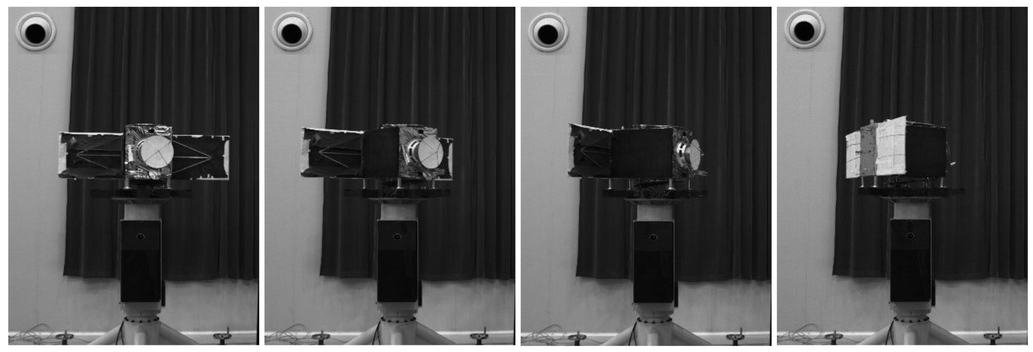
In order to test the real performance of the algorithm, a field experiment was carried out. The satellite model with a 1:6 scale, shown in Figure 15, was fixed on a 6-DOF turntable, and the model can follow the turntable to make a rotary motion about the fixed axis. The control precision of the turntable is .
The measurement sensor is a single-line scanning 3D-LIDAR (Time-of-Flight) system developed by BICE and the point cloud acquisition frequency is greater than 10 Hz.
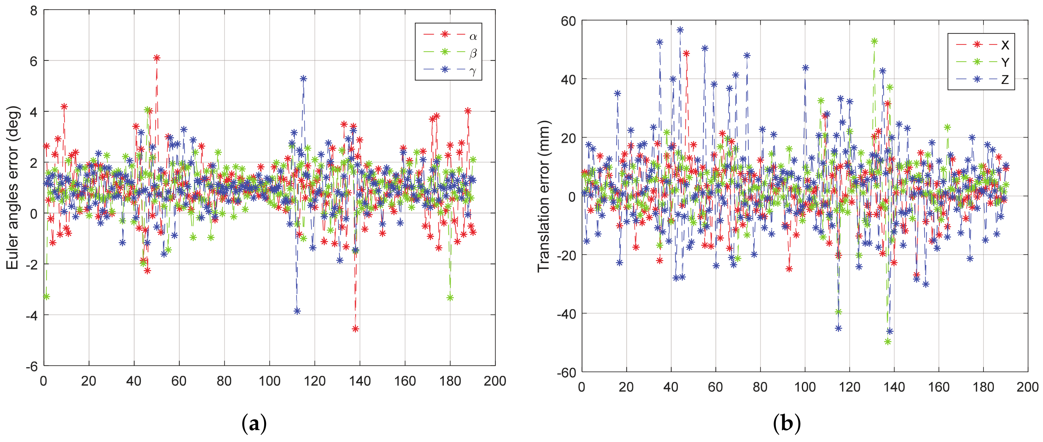
When the target rotates continuously, the points outside the target cannot be easily removed. Therefore, only the experiment about rotating around the y-axis is performed. Based on known information such as the distance between the target and the wall, we can filter out the noise outside the model that does not appear in space. Turntable rotation speed is set to be /s, the frequency of point cloud data acquisition is set to be 10 Hz. In this experiment, the target only rotates around the y-axis without translation. The experimental results are as shown in Figure 16.
From Figure 16, we can see that both the rotation error and the translation error of the field experiment are increased compared with the results of simulation experiments. The reason is that the measurement error of LIDAR itself is more complicated than the simulation error, and the rotation of the target also leads to the deformation of the point cloud data. However, the overall result still shows good accuracy and stability; the rotation error is almost less than , and the translation error is almost less than 20 mm.
6. Conclusions
In this paper, a high accuracy, good real-time and reliable initial pose determination method CTA, which can be used for sparse unordered LIDAR data, is proposed to provide a reliable initial value for tracking. Based on the known target model, this method uses the congruent tetrahedron approach to estimate relative pose, and then uses ICP algorithm for pose tracking. The two main parameters that affect the CTA algorithm are analyzed in detail. The 3D target model point cloud should be resampled as uniform as possible, and there is a speed/accuracy tradeoff when the value nears to the point cloud interval value which have been verified in the subsequent simulation experiments. At the same time, the numerical simulated experiments are completed in a variety of attitudes by artificially adding noise. The results denote that the proposed CTA algorithm is accurate, efficient and robust. The results of numerical simulated experiments and field experiments, which simulate the motion of a high-speed spinning target, demonstrate that the proposed method CTA to estimate the Initial pose and ICP method to track pose can satisfy the real-time calculation of 6-DOF pose of high-speed tumbling target system.
In addition, the LIDAR point cloud in this algorithm can be very sparse and unorganized. The method also can be used for dense point cloud only if the down sampling is used to reduce the time off establishing the convex hull, to ensure the real-time performance of the algorithm. Therefore, it is suitable for other types of LIDAR systems, such as flash LIDAR.
In future work, the robustness of the CTA algorithm will be analyzed considering the different shape and various kinematic states of the targets. In addition, the situation in which the target is occluded also needs to be considered in future work.
Acknowledgments
This work was supported by the National Natural Science Foundation of China (Grant No. 61633002) and the Space Research Program (No. 30508020204HT02). Our grateful thanks are to Junkai Wu and Wei Gao for assisting the implementation of the simulation system and to Mingjie Dong for assisting in the conception of the experiments.
Author Contributions
The work presented in this paper corresponds to a collaborative development by all authors. F.Y. and Y.W. defined the research line; F.Y. and S.X. conceived and designed the experiments. F.Y. and Y.W. performed the experiments and analyzed the data; F.Y. implemented the system and wrote the paper. W.C. supervised the whole work. F.Y., W.C. and G.Y. revised the manuscript.
Conflicts of Interest
The authors declare no conflict of interest.
References
- Flores-Abad, A.; Ma, O.; Pham, K.; Ulrich, S. A review of space robotics technologies for on-orbit servicing. Prog. Aeosp. Sci. 2014, 68, 1–26. [Google Scholar] [CrossRef]
- Tatsch, A.; Fitz-Coy, N.; Gladun, S. On-orbit servicing: A brief survey. In Proceedings of the 2006 Performance Metrics Intelligent Systems Workshop, Gaithersburg, MD, USA, 21–23 August 2006; pp. 276–281. [Google Scholar]
- Bonnal, C.; Ruault, J.M.; Desjean, M.C. Active debris removal: Recent progress and current trends. Acta Astronaut. 2013, 85, 51–60. [Google Scholar] [CrossRef]
- Zhang, H.; Jiang, Z.; Elgammal, A. Vision-based pose estimation for cooperative space objects. Acta Astronaut. 2013, 91, 115–122. [Google Scholar] [CrossRef]
- Wang, X.; Şekercioğlu, Y.A.; Drummond, T. Vision-Based Cooperative Pose Estimation for Localization in Multi-Robot Systems Equipped with RGB-D Cameras. Robotics 2014, 4, 1–22. [Google Scholar] [CrossRef]
- Christian, J.A.; Robinson, S.B.; DŚouza, C.N.; Ruiz, J.P. Cooperative relative navigation of spacecraft using flash light detection and ranging sensors. J. Guid. Control Dyn. 2014, 37, 452–465. [Google Scholar] [CrossRef]
- Weismuller, T.; Leinz, M. GN&C technology demonstrated by the orbital express autonomous Rende vous and capture sensor system. In Proceedings of the 29th Annual American Astronautical Society Guidance and Control Conference, Breckenridge, CO, USA, 4–8 February 2006. [Google Scholar]
- Bodin, P.; Noteborn, R.; Larsson, R.; Karlsson, T.; DÁmico, S.; Ardaens, J.S.; Ardaens, J.-S.; Delpech, M.; Berges, J.-C. Prisma Formation Flying Demonstrator: Overview and Conclusions from the Nominal Mission. In Proceedings of the 35th Annual American Astronautical Society Guidance and Control Conference, Breckenridge, CO, USA, 3–8 February 2012; pp. 441–460. [Google Scholar]
- Volpe, R.; Sabatini, M.; Palmerini, G.B. Pose and Shape Reconstruction of a Noncooperative Spacecraft Using Camera and Range Measurements. Int. J. Aerosp. Eng. 2017, 2017. [Google Scholar] [CrossRef]
- Volpe, R.; Palmerini, G.B.; Sabatini, M. Monocular and lidar based determination of shape, relative attitude and position of a non-cooperative unknown satellite. In Proceedings of the 68th International Astronautical Congress 2017, Adelaide, Australia, 25–29 September 2017. [Google Scholar]
- Woods, J.O.; Christian, J.A. Lidar-based relative navigation with respect to non-cooperative objects. Acta Astronaut. 2016, 126, 298–311. [Google Scholar] [CrossRef]
- Besl, P.D.; McKay, N.D. A Method for Registration of 3-D Shapes. IEEE Trans. Pattern Anal. Mach. Intell. 1992, 14, 239–256. [Google Scholar] [CrossRef]
- Ning, M.; Zhang, S.; Wang, S. A Non-Cooperative Satellite Feature Point Selection Method for Vision-Based Navigation System. Sensors 2018, 18, 854. [Google Scholar] [CrossRef] [PubMed]
- D’Amico, S.; Benn, M.; Jørgensen, J.L. Pose estimation of an uncooperative spacecraft from actual space imagery. Int. J. Space Sci. Eng. 2014, 2, 171–189. [Google Scholar]
- Cai, J.; Huang, P.; Zhang, B.; Wang, D. A TSR Visual Servoing System Based on a Novel Dynamic Template Matching Method. Sensors 2015, 15, 32152–32167. [Google Scholar] [CrossRef] [PubMed]
- Lepetit, V.; Moreno-Noguer, F.; Fua, P. Epnp: An accurate o(n) solution to the pnp problem. Int. J. Comput. Vis. 2009, 81, 155–166. [Google Scholar] [CrossRef] [Green Version]
- Kneip, L.; Scaramuzza, D.; Siegwart, R. A novel parametrization of the perspective-three-point problem for a direct computation of absolute camera position and orientation. In Proceedings of the 24th IEEE Conference on Computer Vision and Pattern Recognition, Colorado Springs, CO, USA, 20–25 June 2011; pp. 2969–2976. [Google Scholar]
- Zheng, Y.; Kuang, Y.; Sugimoto, S.; Astrom, K. Revisiting the PnP Problem: A Fast, General and Optimal Solution. In Proceedings of the 2013 IEEE International Conference on Computer Vision, Sydney, NSW, Australia, 3–6 December 2013; pp. 2344–2351. [Google Scholar]
- Dufour, R.M.; Miller, E.L.; Galatsanos, N.P. Template Matching Based Object Recognition with Unknown Geometric Parameters. IEEE Trans. Image Process. 2002, 11, 1385–1396. [Google Scholar] [CrossRef] [PubMed]
- David, P.; Dementhon, D.; Duraiswami, R.; Samet, H. Softposit: Simultaneous pose and correspondence determination. Int. J. Comput. Vis. 2004, 59, 259–284. [Google Scholar] [CrossRef]
- Gold, S.; Rangarajan, A. A graduated assignment algorithm for graph matching. IEEE Trans. Pattern Anal. Mach. Intell. 1996, 18, 377–388. [Google Scholar] [CrossRef]
- Gold, S.; Rangarajan, A.; Lu, C.-P.; Pappu, S.; Mjolsness, E. New algorithms for 2D and 3D point matching: Pose estimation and correspondence. Pattern Recognit. 1998, 31, 1019–1031. [Google Scholar] [CrossRef]
- DeMenthon, D.; Davis, L.S. Model-based object pose in 25 lines of code. Int. J. Comput. Vis. 1995, 15, 123–141. [Google Scholar] [CrossRef]
- Jasiobedzki, P.; Se, S.; Pan, T.; Umasuthan, M.; Greenspan, M. Autonomous satellite rendezvous and docking using LIDAR and model based vision. In SPIE Spaceborne Sensor II; SPIE: Bellingham, WA, USA, 2005. [Google Scholar] [CrossRef]
- Sommer, I. Ahrns, GNC for a rendezvous in space with an uncooperative target. In Proceedings of the 5th International Conference on Spacecraft Formation Flying Missions and Technologies, Munich, Germany, 29–31 May 2013; pp. 1–15. [Google Scholar]
- Opromolla, R.; Fasano, G.; Rufino, G.; Grassi, M. Uncooperative pose estimation with a LIDAR-based system. Acta Astronaut. 2015, 110, 287–297. [Google Scholar] [CrossRef]
- Opromolla, R.; Fasano, G.; Rufino, G.; Grassi, M. A model-based 3D template matching technique for pose acquisition of an uncooperative space object. Sensors 2015, 15, 6360–6382. [Google Scholar] [CrossRef] [PubMed]
- Opromolla, R.; Fasano, G.; Rufino, G.; Grassi, M. Pose Estimation for Spacecraft Relative Navigation Using Model-based Algorithms. IEEE Trans. Aerosp. Electron. Syst. 2017, 53, 431–447. [Google Scholar] [CrossRef]
- Aldoma, A.; Tombari, F.; Rusu, R.B.; Vincze, M. OUR-CVFH: Oriented, Unique and Repeatable Clustered Viewpoint Feature Histogram for Object Recognition and 6DOF Pose Estimation. In Pattern Recognition; Springer: Berlin, Germany, 2012. [Google Scholar]
- Liu, L.; Zhao, G.; Bo, Y. Point Cloud Based Relative Pose Estimation of a Satellite in Close Range. Sensors 2016, 16, 824. [Google Scholar] [CrossRef] [PubMed]
- Yang, J.; Li, H.; Jia, Y. Go-ICP: Solving 3D registration efficiently and globally optimally. In Proceedings of the 2013 IEEE International Conference on Computer Vision, Sydney, NSW, Australia, 3–6 December 2013; pp. 1457–1464. [Google Scholar]
- Hartley, R.I.; Kahl, F. Global optimization through rotation space search. Int. J. Comput. Vis. 2009, 82, 64–79. [Google Scholar] [CrossRef]
- Ruel, S.; Luu, T.; Anctil, M.; Gagnon, S. Target localization from 3D data for on-orbit autonomous rendezvous and docking. In Proceedings of the 2008 IEEE Aerospace Conference, Big Sky, MT, USA, 1–8 March 2008; pp. 1–11. [Google Scholar]
- Barber, C.B.; Dobkin, D.P.; Huhdanpaa, H. The quickhull algorithm for convex hulls. ACM Trans. Math. Softw. 1996, 22, 469–483. [Google Scholar] [CrossRef]
- Barber, C.B.; Dobkin, D.P.; Huhdanpaa, H. Qhull: Quickhull Algorithm for Computing the Convex Hull; Astrophysics Source Code Library: Houghton, MI, USA, 2013; record ascl:1304.016. [Google Scholar]
- Chand, D.R.; Kapur, S.S. An Algorithm for Convex Polytopes. J. ACM 1970, 17, 78–86. [Google Scholar] [CrossRef]
- Cintra, M.; Llanos, D.R.; Palop, B. Speculative Parallelization of a Randomized Incremental Convex Hull Algorithm. In Proceedings of the 2004 International Conference on Computational Science and its Applications, Assisi, Italy, 14–17 May 2004; pp. 188–197. [Google Scholar]
- English, C.; Okouneva, G.; Saint-Cyr, P.; Choudhuri, A.; Luu, T. Real-time dynamic pose estimation systems in space: Lessons learned for system design and performance evaluation. Int. J. Intell. Control Syst. 2011, 16, 79–96. [Google Scholar]
Figure 1.
Logical scheme of the proposed method for relative pose determination.

Figure 2.
The definition of reference frames [30].
Figure 2.
The definition of reference frames [30].

Figure 3.
Flow of CTA Algorithm.

Figure 4.
Building the two-level index hash table.

Figure 5.
Logic of successful pose estimation for the CTA algorithms.

Figure 6.
A small incurring a failure of finding a corresponding point.

Figure 7.
A large introducing redundant candidates.

Figure 8.
The 3D point cloud simulation software (a) Lissajous, (b) Rosette, (c) Spiral.

Figure 9.
Performance of congruent tetrahedron align algorithm. (a) CDF of rotation error; (b) CDF of translation error; (c) CDF of processing time.
Figure 9.
Performance of congruent tetrahedron align algorithm. (a) CDF of rotation error; (b) CDF of translation error; (c) CDF of processing time.

Figure 10.
Three different initial attitudes of numerical simulated experiments. (a) ; (b) ; (c) .

Figure 11.
The error curve of (a) rotation and (b) translation of test 1.

Figure 12.
The error curve of (a) rotation and (b) translation of test 2.

Figure 13.
The error curve of (a) rotation and (b) translation of test 3.

Figure 14.
The error curve of (a) rotation and (b) translation of test 4.

Figure 15.
Field experiment.

Figure 16.
The error curve of (a) rotation and (b) translation of field experiment.


Table 1.
The average estimation pose error of different .
| binNum | Time/ms | Points Num | X/mm | Y/mm | Z/mm | Error Rate/% | |||
|---|---|---|---|---|---|---|---|---|---|
| 5 | 28,752.59 | 102 | 1.36 | 1.60 | 0.50 | 23.53 | 81.40 | 81.82 | 0 |
| 10 | 1703.99 | 102 | 1.53 | 1.58 | 0.52 | 25.04 | 75.07 | 85.24 | 0 |
| 15 | 221.18 | 102 | 1.92 | 1.63 | 0.51 | 27.00 | 70.12 | 92.00 | 0 |
| 20 | 62.24 | 102 | 1.76 | 1.92 | 0.51 | 27.16 | 75.03 | 85.45 | 0 |
| 25 | 33.27 | 102 | 1.77 | 1.55 | 0.54 | 24.98 | 86.77 | 81.04 | 2.8 |
| 30 | 17.23 | 102 | 1.72 | 1.77 | 0.53 | 25.63 | 75.01 | 83.10 | 5.7 |
| 35 | 17.17 | 102 | 1.50 | 1.78 | 0.53 | 22.45 | 85.64 | 95.75 | 11.4 |
| 40 | 15.11 | 102 | 1.30 | 1.46 | 0.49 | 21.34 | 96.88 | 72.48 | 25.7 |
| 50 | 14.98 | 103 | 1.46 | 1.41 | 0.56 | 22.79 | 88.69 | 89.51 | 34.3 |
| 60 | 13.14 | 104 | 1.60 | 1.52 | 0.37 | 19.16 | 69.69 | 71.50 | 60 |
| 70 | 14.49 | 106 | 2.78 | 2.01 | 0.55 | 23.17 | 94.40 | 60.70 | 85.7 |
| 80 | 13.95 | 105 | 2.03 | 1.58 | 0.52 | 26.64 | 89.31 | 76.10 | 80 |
© 2018 by the authors. Licensee MDPI, Basel, Switzerland. This article is an open access article distributed under the terms and conditions of the Creative Commons Attribution (CC BY) license (http://creativecommons.org/licenses/by/4.0/).
Share and Cite
MDPI and ACS Style
Yin, F.; Chou, W.; Wu, Y.; Yang, G.; Xu, S. Sparse Unorganized Point Cloud Based Relative Pose Estimation for Uncooperative Space Target. Sensors 2018, 18, 1009. https://doi.org/10.3390/s18041009
AMA Style
Yin F, Chou W, Wu Y, Yang G, Xu S. Sparse Unorganized Point Cloud Based Relative Pose Estimation for Uncooperative Space Target. Sensors. 2018; 18(4):1009. https://doi.org/10.3390/s18041009
Chicago/Turabian StyleYin, Fang, Wusheng Chou, Yun Wu, Guang Yang, and Song Xu. 2018. "Sparse Unorganized Point Cloud Based Relative Pose Estimation for Uncooperative Space Target" Sensors 18, no. 4: 1009. https://doi.org/10.3390/s18041009
Note that from the first issue of 2016, this journal uses article numbers instead of page numbers. See further details here.