Using a Mobile Device “App” and Proximal Remote Sensing Technologies to Assess Soil Cover Fractions on Agricultural Fields

Abstract

Quantifying the amount of crop residue left in the field after harvest is a key issue for sustainability. Conventional assessment approaches (e.g., line-transect) are labor intensive, time-consuming and costly. Many proximal remote sensing devices and systems have been developed for agricultural applications such as cover crop and residue mapping. For instance, current mobile devices (smartphones & tablets) are usually equipped with digital cameras and global positioning systems and use applications (apps) for in-field data collection and analysis. In this study, we assess the feasibility and strength of a mobile device app developed to estimate crop residue cover. The performance of this novel technique (from here on referred to as “app” method) was compared against two point counting approaches: an established digital photograph-grid method and a new automated residue counting script developed in MATLAB at the University of Guelph. Both photograph-grid and script methods were used to count residue under 100 grid points. Residue percent cover was estimated using the app, script and photograph-grid methods on 54 vertical digital photographs (images of the ground taken from above at a height of 1.5 m) collected from eighteen fields (9 corn and 9 soybean, 3 samples each) located in southern Ontario. Results showed that residue estimates from the app method were in good agreement with those obtained from both photograph–grid and script methods (R² = 0.86 and 0.84, respectively). This study has found that the app underestimates the residue coverage by −6.3% and −10.8% when compared to the photograph-grid and script methods, respectively. With regards to residue type, soybean has a slightly lower bias than corn (i.e., −5.3% vs. −7.4%). For photos with residue <30%, the app derived residue measurements are within ±5% difference (bias) of both photograph-grid- and script-derived residue measurements. These methods could therefore be used to track the recommended minimum soil residue cover of 30%, implemented to reduce farmland topsoil and nutrient losses that impact water quality. Overall, the app method was found to be a good alternative to the point counting methods, which are more time-consuming.

1. Introduction

The amount of crop residue left in the field after harvest is of great importance for water storage [1], soil erosion control [2,3,4] and assessment and modeling of soil carbon sequestration [5]. Retaining crop residue is of interest in agro-ecosystems in North America, such as the mid-West and Great Lakes states where agricultural practices, including tillage practices (preparing land for growing crops), can affect water quality of the Gulf of Mexico and Great Lakes [6]. Such practices are of greater importance in the Canadian agro-ecosystem of southwestern Ontario, an area where, retaining crop residue cover ≥30% on the surface is considered a conservation tillage practice [7,8,9] and is an important objective of the Great Lakes Agricultural Stewardship Initiative funded by Agriculture and Agri-food Canada (AAFC) and the Ontario Ministry of Agriculture, Food and Rural Affairs (OMAFRA, [10]). Previous studies have found that conservation tillage and crop residue cover are important for reducing time and fuel consumption, improving water and soil quality [11,12,13], increasing the amount of organic matter [14,15,16], reducing greenhouse gas emissions [17] and reducing soil erosion by up to 75% by maintaining a corn crop residue cover of 15% [18]. Crop residue cover estimation has been used to qualify specific fields for federal or provincial conservation programs (i.e., Land Stewardship I and II Programs offered by OMAFRA from 1987 to 1994). Such quantitative information on the amount of crop residue cover by field, which can then be extrapolated to regions, is essential to understand the state of soil management and the capacity for additional change in an area of interest.

The ability of tillage and planting systems to maintain soil residue cover is currently measured by using one or more of the following methods: Line-transect method (e.g., knotted rope), Meter stick method, Photograph comparison method, Calculation method and Photographic-grid method. Each of these techniques, described more completely by Dodd et al. [19], has various advantages and disadvantages. A common feature of each, however, is that they tend to be laborious and time-consuming to complete properly. These might be reasons why few landowners directly measure their field residue levels. Line-transect and digital photograph-grid methods are the two main approaches that have been widely used to quantify crop residue cover from ground observations. However, the standard ground-based line-transect method requires significant effort to collect an optimal number of samples [20], is time consuming, labor intensive and cannot provide continuous data over large areas, as percent residue cover is estimated at spatially and temporally disconnected fields. Several studies have found that the digital photograph-grid method can be a suitable alternative to the line-transect method (i.e., [5,20]). However, one of the main issues in the use of photographs to derive percent residue cover is that multiple manipulations are required (i.e., photograph collection, grid preparation, visual counting by different observers, script or spreadsheet calculation of percentage cover). Remote sensing imagery is a valuable tool to assess and map tillage practices, crop residue cover and cover crops over large areas. However, monitoring and deriving information on crop residue cover from space has been restricted in the past by low spectral and spatial-temporal resolution and availability of ground truth data [21]. Therefore, there is a need to identify low-cost, reliable, quick and easy to implement methods for residue estimation.

Mobile application technologies are becoming more abundant in farm management around the world. For instance, Dehnen-Schmutz et al. [22] found that 84% of British and French farmers used their smartphone for farm management. In the province of Ontario about 39% of farmers had used their smartphones/tablets for farm management in 2015; 56% had used computers/laptops [23]. The fact that many mobile devices (i.e., smartphones, tablets) have technical components such as GPS, camera and core processing power makes them suitable for several proximal remote sensing purposes. They can offer valuable, accurate and rapid information, calculations, measurements, or evaluations of agriculture attributes. Numerous studies have used mobile device applications (apps) to assess green crop cover [24], ground cover [25], fractional green canopy cover [26], turf coverage [27], leaf area index [28,29], or chlorophyll content in corn plants [30], or citizen science and/or participatory sensing [22,31,32]. One advantage of these devices is that they are equipped with digital cameras and processors, which allow users (i.e., farmers and/or crop advisors) to capture images and perform crop residue analysis efficiently. Despite the increased interest in using proximal remote sensing mobile devices in different agricultural applications, reported attempts to estimate percent crop cover residue using these technologies are limited. Here, we tested and validated a free Crop Residue Estimator (i.e., recently developed by ©FieldTRAKS Solutions [33]) that can be deployed on various platforms including web applications and mobile technologies. This app uses an automated color threshold image classification process method. This method requires the selection of pixels (RGB) that represent the target object (i.e., residue cover or soil surface). The image is classified using the onboard processing capabilities of the device and is based upon a histogram of selected RGB pixel values. The method produces a 2-class thematic image representing either crop residue or soil surface. The pixels of each class are summed to determine the percent cover. One advantage of this method is that the mobile device returns immediate results which may be saved to create a statistical summary. FieldTRAKS Solutions created this application as a proof of concept and this is the first time that it has been tested in a comparison with an accepted method of calculating crop residue to evaluate its performance before it can be broadly recommended.

The objectives of this paper are to test the feasibility and strength of this mobile device app in assessing residue cover and to qualitatively compare this new method’s performance against existing ground survey techniques. Specifically, we compared the residue cover estimates derived from the “app” method to those obtained using digital photograph-grid method and an automated residue counting script procedure. In a recent study [20], the photograph-grid method was found strongly correlated to the line-transect method which is considered a standard and robust method for assessing crop residue and was the “ground truth” in the context of that study. In this study, both photograph-grid and script methods were used to count residue under 100 grid points and are considered as reference methods in this evaluation. The three methods (app, photograph-grid and script) were evaluated using the same digital photograph dataset. The ultimate goal is to demonstrate if using a proximal remote sensing mobile device with a color threshold app can be a convenient alternative to methods that use digital photograph intersection counting for crop residue cover assessment.

2. Materials and Methods

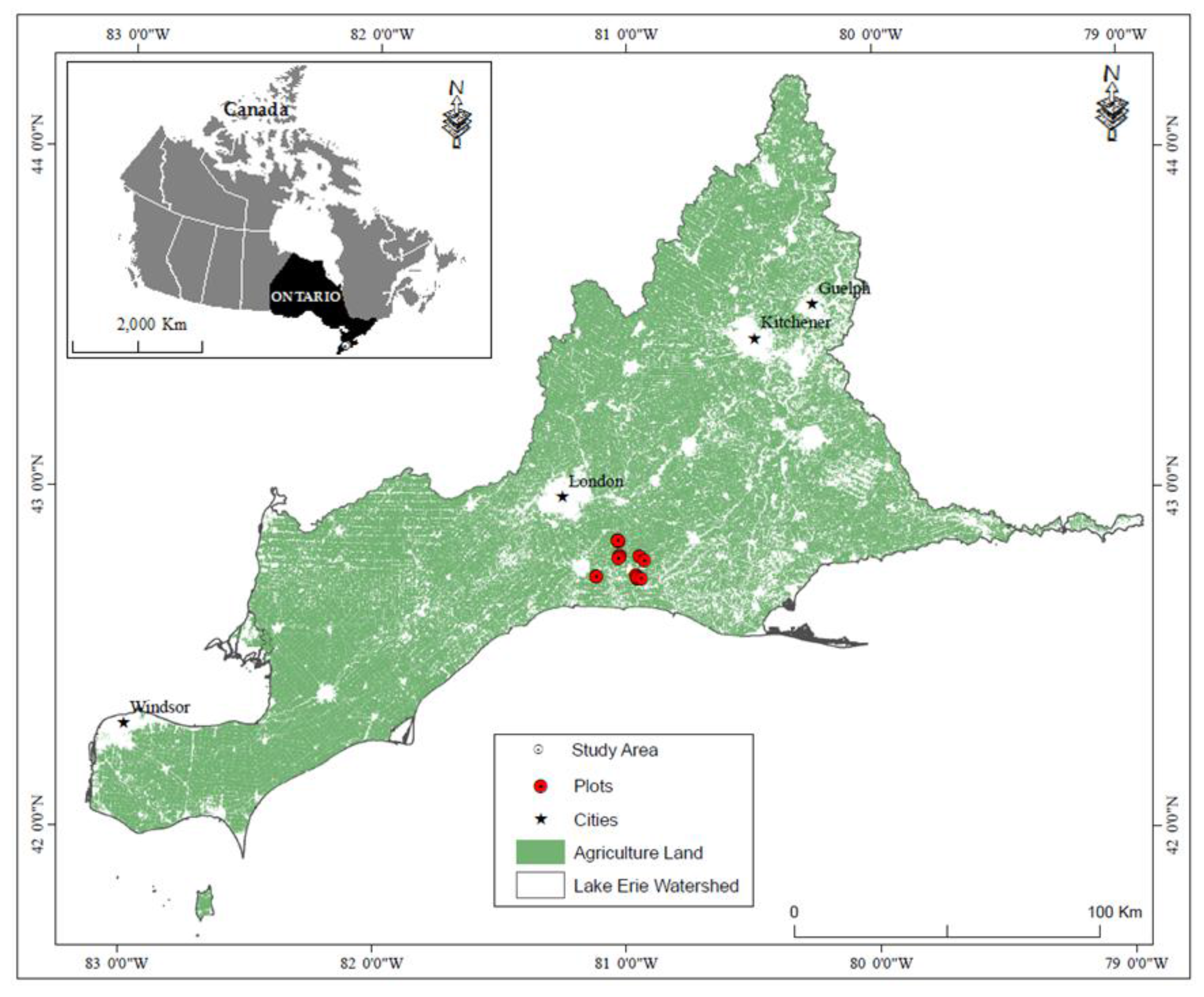
2.1. Study Area

This study is conducted within the Lake Erie basin of southwestern Ontario, Canada (Figure 1). This area is primarily agricultural, with corn (Zea mays), soybean (Glycine max) and winter wheat (Triticum aestivum L.) as the dominant crops grown in rotation in this region. The topography is generally characterized by a combination of flat and rolling terrain, occasionally interspersed with steep ravines. Soils in the sample area range in texture from clay loam to loamy sand. The southwestern region of Ontario has the largest tillable land area in the province with a total of 3,026,576 ha [34] and an estimated biomass of residue (from three common crops, i.e., corn, soybean and winter wheat) that could be removed annually ranging between 6963 and 7223 kg/ha [35]. The area has a climate typically characterized by long moderate winters (November–April) and hot and humid summers. The average annual temperature is 8.7 °C with June, July and August as the warmest months (mean of 20.1 °C); and December, January and February as the coldest months (mean of –3.2 °C). Total annual precipitation is 993 mm, of which about one-third falls during the peak vegetative growth period, between early May and August (Environment Canada, 2011; St. Thomas weather station, about 15 km W of the study area). The bulk of the precipitation (2/3) falls during the non-growing season as fall or spring rain, or winter snow which then leaves the landscape after melting during winter thaw periods or as spring runoff. This is of significance as it means that the bulk of the precipitation occurs during the non-growing season when the landscape is most vulnerable to soil erosion; this emphasizes why retaining sufficient crop residue cover is an important and effective soil management practice in this region [6].

2.2. Sampling Design and Field Data Collection Field

Our study involved fields that had been established as part of a larger project that dealt with the use of multi-temporal remote sensing for mapping and quantification of soil cover on southern Ontario agricultural fields over the Lake Erie basin (see Figure 1 and [20]). Eighteen square plots (one 15 m × 15 m plot per field) were established throughout the study area and sampled in fall 2014 after harvest. These 18 separate agricultural fields were located on privately-owned farms. The harvested crops on these 18 plots were corn (9 plots) and soybean (9 plots); and three samples (i.e., three photographs) per plot were collected. We aimed to sample three residue levels from each crop a priori from a visible assessment (i.e., 3 low residue corn, 3 low soybean, 3 medium corn, 3 medium soybean, 3 high corn and 3 high soybean where: low: <30%, medium: 30–60% and high: >60% residue cover respectively); fields were assigned to the appropriate category after they were measured, resulting in more samples in the low residue category (22) and fewer in the medium (15) and high (17) residue categories than originally planned (18 samples each).

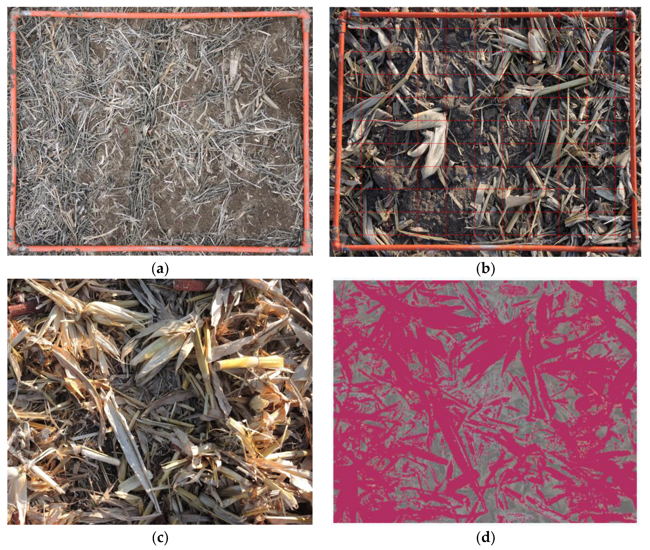
2.2.1. Photograph-Grid Method

In a recent study, we have found that percentage of crop residue estimates derived from either five or three digital photographs per plot were both strongly correlated to those derived from a reference method (i.e., line-transect). Therefore, among the 5 photos used in that study [20], only three photographs per plot were randomly selected and used here, for a total of 54 photographs. These 54 photographs (three per plot), were taken using a digital camera (i.e., Nikon COOLPIX P7800 12.2 MP Digital Camera with 7.1× Optical Zoom, China). At each plot, photos were taken at a 90-degree angle to the ground (perpendicular to soil surface) as this orientation is preferable for soil cover assessment [36] and at a fixed height (1.5 m). To do so, a 75 × 100 cm quadrat was placed on the ground with its longest side perpendicular to tillage direction, or planting direction if there was no tillage (Figure 2a). Once photographs of the quadrat were taken, percent residue cover from those photographs was derived using a uniformly spaced 10 by 10 digital grid (i.e., 100 intersections; Figure 2b). To do so, first, the digital grid was super-imposed on each digital photograph, as in [5,20,21], so that the grid spans the majority of the photo. The grid-line thickness was matched to that of a wooden dowel specification (≥3/32 inches or ≥0.24 cm in diameter) following Shelton et al.’s [37] method using the scale of the quadrat. Second, intersections of residue with the grid were counted visually from a computer screen and percent cover was then calculated as the percent of total intersections that overlay residue.

2.2.2. App Method

The same set of 54 photographs was downloaded to an Android tablet and analyzed for crop residue cover using a mobile application technology. The app used in this study was developed by FieldTRAKS Solutions Inc. [33] and was partially funded through the Ontario Water Resource Adaptation and Management Initiative (2013). It was developed as a hybrid application using the Adobe PhoneGap cross-platform framework which aims to combine the convenience of developing with HTML5, JavaScript and CSS with the power of the native apps access to device’s the APIs and sensors. FieldTRAKS Solutions views the application to be a prototype or proof of concept and has made it freely available in its’ present form as an APK install for Android device (available for download at www.fieldtraks.ca). It employs an in-house crop residue image analysis algorithm that can be deployed in various platforms including web application and mobile technologies. This technique creates an automated color threshold image classification based on RGB pixel values only (i.e., without any normalization) through the selection of points (i.e., training dataset) which are representative of the target crop residue of the current processed digital photograph. The processing algorithm creates a histogram of RGB color values and selects values that fall within the color ranges created by selecting representative pixels of the target (e.g., corn residue or soybean residue). The histogram and target values are relative to the current image and no adjustments were made for shadows or any other sun effects. It is assumed that any such effects will be consistent throughout the image and affect target and non-target areas equally as all photos were taken under the same illumination conditions. As points are selected, an internal histogram of RGB values is constructed that represents the colour ranges of the crop residue in the image. Pixels with RGB values outside of the histogram are viewed to be soil or non-crop residue material. For the purposes of this study, sampling points of residue were chosen on every photo and used as training to direct the image processing software for the classification of all other pixels in the digital photo.

No optimal number of sampling points was provided by the app developer but an arbitrary minimum of four training sample points on each photo was suggested. To determine the appropriate number to be used as reference for this study, we tested multiple numbers of sampling points (i.e., 4, 8, 12) and have found that an increase in the number of sampling points (i.e., 4 to 12) is associated with a notable decrease of the correlation coefficient (data not shown) between residue percent derived from photograph-grid and app methods, leading to an overestimation of the residue percent. Nevertheless, four and eight sampling points had lower overestimation of the residue percent. Therefore, four to eight different sample residue pieces (i.e., training points) per photo were used for this study. Generally, a minimum of four sampling points were selected if the residue was homogeneous with respect to contrast and colour and more (i.e., maximum of 8) were selected in the more heterogeneous cases. The following selection procedures/guidelines were used to optimize the residue colour selection and capture variation across the photo for the 4–8 sample points selected: (i) the sampling points were selected from across all the image and not from one corner; (ii) in each photo, the brightest and the darkest pieces of residue, then a mix of larger and smaller piece of residue had to be chosen; and (iii) if more than one type of crop residue (i.e., soybean and corn) is present in the photo, each type of residue (darkest and brightest) was selected. It is important to mention that photos with >60% residue cover required selection of the maximum number of points (i.e., up to 8), whereas photos with less than 30% residue had a narrower range of residue colours and thus required fewer points selected (i.e., minimum 4).

Once all the sampling points were chosen (Figure 2c), the classification analysis was performed by the app and the estimated crop residue was displayed as a percentage on the tablet screen together with a thematic classified image (Figure 2d) using a two-color palette legend (residue and no-residue classes).

2.2.3. Residue Cover Obtained from Digital Photograph-Grid Counting and the App Classification

Similar to a pre-established set of rules used in a recent study [20], the residue cover percent for each digital photograph for both the photograph-grid and app methods was determined by an average of two assessors. To begin, independent assessments by three persons were carried out on a photo using each method. When the estimates of a minimum of two persons for a method were within ±5% difference of the residue estimate of an individual photograph (i.e., either photograph-grid or the app counting), the two estimates with the smallest difference were averaged and used as the photograph’s and app’s datum. When assessments by all three persons disagreed by >5%, the estimate provided by the most accurate person (considered the counter with the most experience) was averaged with the estimate of the second counter in closest agreement with the most accurate estimate. Estimates from only two persons, for each photo, were averaged in order to minimize the human error that might affect the counting process and to increase the accuracy of the estimated percent crop residue cover.

2.2.4. Crop Residue Cover Estimation Using the Script Method

In addition to the photograph-grid method and the app method, a MATLAB script developed at the University of Guelph in 2016 was tested on the same set of 54 photographs. The script method aims to make the residue counting procedure more accurate, efficient, semi-automatic, rapid and transparent. As in Booth et al. (2006), the script method automates the manual pixel classification (MPC) procedure and the ensuing analysis, while only using the keyboard’s arrow keys. On the other hand, manual pixel classification methods are particularly useful when calibrating automatic color threshold methods (Booth et al. 2006; i.e., the app). The script method was conducted by overlaying a 10 by 10 digital grid (for a total of 100-intersection) on each digital photograph, as in [5,20,21]. It is important to mention that a script with a denser grid (i.e., 400-intersections) was also tested on the same 54 photographs to evaluate whether this would substantially improve the correlation coefficient between the app and script results. This quadrupling in sample size led to a marginal increase in the coefficient of determination (0.84 vs. 0.82) while increasing the evaluation time four-fold. The script has the advantages of automating the overlay of grid intersections so there is less photo manipulation of creating a record of the classification decisions.

Before running the script on every photograph, each of the 100 grid intersections was identified with a centered red circular marker; once classified the marker turns either green, indicating residue, or black, indicating no residue. The crosshairs, created by the grid intersection and circular marker, allow for greater viewing of both adjacent pixels and the sample pixel using keyboard symbols. The script automatically locates and zooms in (2×) on the grid intersections, where the user records whether the pixel contains residue (↓) or not (→), the user also has the option to zoom in (↑) up to 32× or reclassify to the previous intersection (←). The zoom function repeats the original image pixels in two dimensions to yield the visual effect of the single square pixel growing but not changing in color or sharpness. The user is taken from one point to the next until each intersection is classified. The script also automates the calculation of the image percent cover and estimates error statistics (based on a binomial distribution). The number and location of intersections classified as residue is automatically recorded and the script outputs a spreadsheet for each photo, listing the intersection coordinates and classification decision, a low-resolution duplicate of the photo showing the classification decisions at each intersection and a meta-spreadsheet that tabulates the results for each image analyzed. Only one person’s assessment was used for the script-method to determine percent residue.

2.3. Statistical Analysis

Crop residue cover estimates derived from both digital photograph counting methods and the app were compared using linear regression models. Accuracy measures included the coefficient of determination (R²), root mean squared error (RMSE; Equation (1)) and Bias (Equation (2)). R² was used to explore the strength of the relationship between crop residue measured by the different methods, while RMSE was used to determine the magnitude of error among the methods. Bias is a quantitative term describing the difference between the average of measurements from reference method (i.e., photograph-grid and script) and the app method made on the same dataset of photos. RMSE and Bias were determined from Equations (1) and (2) cited in Molinier et al. [32].

$$RMSE=\sqrt{{\displaystyle \sum }_i\frac{{\left(y_i- {\widehat{y}}_i\right)}^2}{n}}$$

(1)

$$BIAS=\frac{{{\displaystyle \sum }}_i\left(y_i- {\widehat{y}}_i\right) }{n}$$

(2)

where y_i is the observed values from digital photograph reference data, ŷ_i represents the app measurements and n the total number of measurements. P-values were determined and significance was declared at α = 0.05. Statistical analyses were conducted in R [38].

As an additional statistical analysis, we also tested whether alternative distributions to model the data could improve the relationships between the methods (app vs. photograph-grid and app vs. script). In this context, non-linear regressions were performed using ordinary least squares (OLS) methods with logarithmic transformations of the response variable (Equation (3)) and logit transformations of the intersection-normalized response variable (Equation (4)).

$$\mathbf{ln}{y}_i={\beta }_0+{\beta }_1{x}_i ⟺ y_i=e^{ {\beta }_0}{e}^{{\beta }_1{x}_i}$$

(3)

$$\mathbf{logit}\left(\frac{y_i}{100}\right)=\mathbf{ln}\left(\frac{y_i/100}{1-\left(y_i/100\right)}\right)={\beta }_0+{\beta }_1{x}_i ⟺ \frac{y_i}{100}=\frac{e^{ {\beta }_0+{\beta }_1{x}_i}}{1+e^{ {\beta }_0+{\beta }_1{x}_i}}$$

(4)

where y_i represent the app measurements, 𝛽₀ and 𝛽₁ are regression coefficients and x_i are the observed values from digital photograph reference data.

Ordinary Least Squares (OLS) regressions are based on the assumption that the response variable is normally distributed; this is not the case for this data set given its discrete and bounded nature. Another assumption of linear regression is homoscedasticity. OLS regression analysis using heteroscedastic data will still provide an unbiased estimate for the relationship between the predictor and response variables but standard errors and therefore inferences obtained from data analysis are suspect. Generalized Poisson [39,40] and Beta Regression [41,42,43] with a logit link function were also used to model the variance of the relationship between the app and both the photograph and script methods. In essence, the log-transformed OLS and Generalized Poisson models establish the relationship between the predictor and response variables similarly but consider the variance using different distributions; the same applies to the logit transformation and the beta regression with a logit link function.

3. Results

3.1. App-, Photograph-Grid and Script-Derived Residue Cover

Table 1. Summary statistics for residue cover percent derived from app, photograph-grid and script methods in the studied 18 plots.

Plot ID	Type	Photograph-Grid-Derived			Script-Derived			App-Derived
		Mean	Range	SE	Mean	Range	SE	Mean	Range	SE
1	CR	4	2–5	0.9	9	3–14	3.3	9	7–13	2.1
2	CR	5	4–6	0.7	12	10–14	1.3	14	12–16	1.3
3	CR	8	4–14	3.1	11	7–19	3.8	6	4–9	1.3
4	CR	47	35–62	8.1	49	39–64	7.6	38	36–40	1.1
5	CR	49	39–68	9.5	54	43–71	8.7	27	21–40	6.4
6	CR	59	41–80	11.3	61	50–73	6.6	43	25–54	9.3
7	CR	74	70–80	2.9	77	72–83	3.2	65	61–73	3.7
8	CR	87	82–92	2.9	81	76–85	2.6	75	62–88	7.7
9	CR	88	74–97	7.2	85	78–90	3.6	77	70–89	6.3
10	SB	7	6–8	0.5	15	12–18	1.8	7	6–7	0.5
11	SB	8	6–10	1.0	18	8–14	1.6	11	8–14	1.6
12	SB	11	4–21	5.1	21	11–34	6.8	11	6–17	3.5
11	SB	12	9–16	2.2	14	10–16	1.9	8	5–9	1.2
14	SB	38	29–48	5.6	41	37–47	3.2	39	20–54	10.2
15	SB	48	42–52	3.1	55	51–58	2.2	32	28–34	1.7
16	SB	58	48–73	7.7	68	62–79	5.4	48	19–72	15.6
17	SB	59	47–70	6.6	68	65–71	1.8	50	43–55	3.6
18	SB	70	54–83	8.5	71	66–80	4.4	58	42–67	8.1

CR = Corn; SB = Soybean; SE refers to Standard Error. Every plot presents the average residue cover percent of three photographs. Plots are cauterized as: Low residue cover (<30%); Medium residue cover (30–60%); or High residue cover (>60%). Plots from fields with <30% and ≥30% residue cover are considered conventional and conservation practices, respectively.

and

Table 2. Summary statistics for residue cover percent grouped by residue type and levels.

Residue	n	Photograph-Grid-Derived			Script-Derived			App-Derived
		Mean	Range	SE	Mean	Range	SE	Mean	Range	SE
All	54	41	2-97	4.1	45	3–90	3.8	34	4–89	3.5
Corn	27	47	2–97	6.5	49	3–90	5.9	39	4–89	5.3
Soybean	27	35	4–83	4.9	41	10–80	4.7	29	5–72	4.3
Low	22	9	2–29	1.3	16	3–38	1.7	11	4–42	1.7
Medium	15	46	35–57	1.7	53	37–66	2.5	35	19–54	3.2
High	17	77	62–97	2.6	77	64–90	1.8	64	38–89	3.4
≥30%	32	63	35–97	3.2	65	37–90	2.6	50	19–89	3.5

SE refers to Standard Error. Residue type level low, medium, and high represent fields with <30%, 30–60%, and >60%, respectively.

show the estimated crop residue as evaluated by app, photograph-grid and script methods in the 18 plots (Table 1) and for the different residue type and levels (Table 2). For the photograph–grid method residue cover ranged from 2–97% for corn (47 ± 6.4%; mean ± Standard Error (SE)) and 6–83% for soybean (35 ± 4.9), while for the app method the percentage of residue cover varied from 4 to 89 for corn (39 ± 5.3%) and 5 to 72 for soybean (29 ± 4.3). For the script method, the corn and soybean range were 3–90% (49 ± 5.9) and 10–80% (41 ± 4.7), respectively. Table 1 also shows that mean residue cover measured for all the data (n = 54) using the app method were on average slightly lower than the photograph-grid- and script-derived measurements (i.e., 34% vs. 41% and 34% vs. 45%, respectively; Table 2).

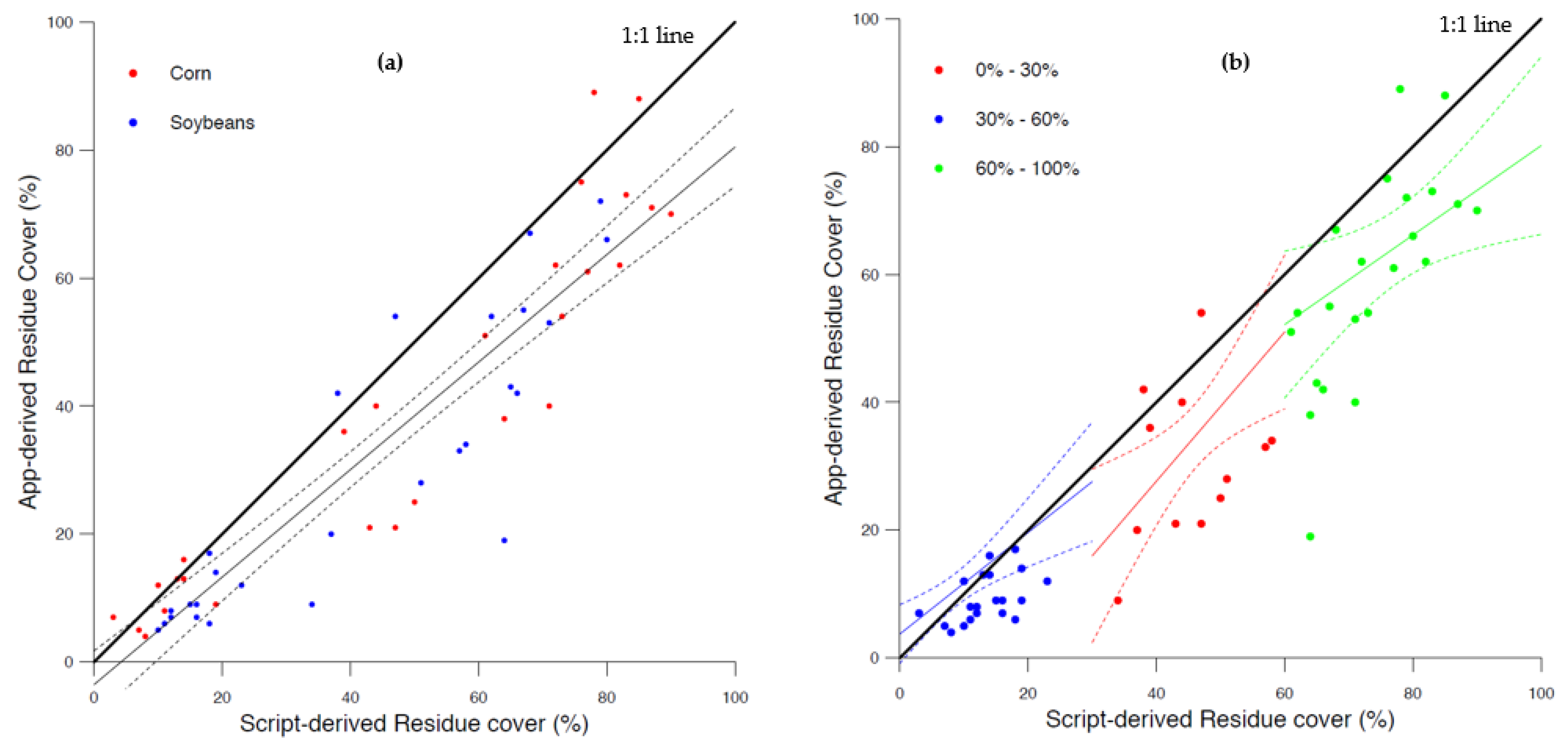
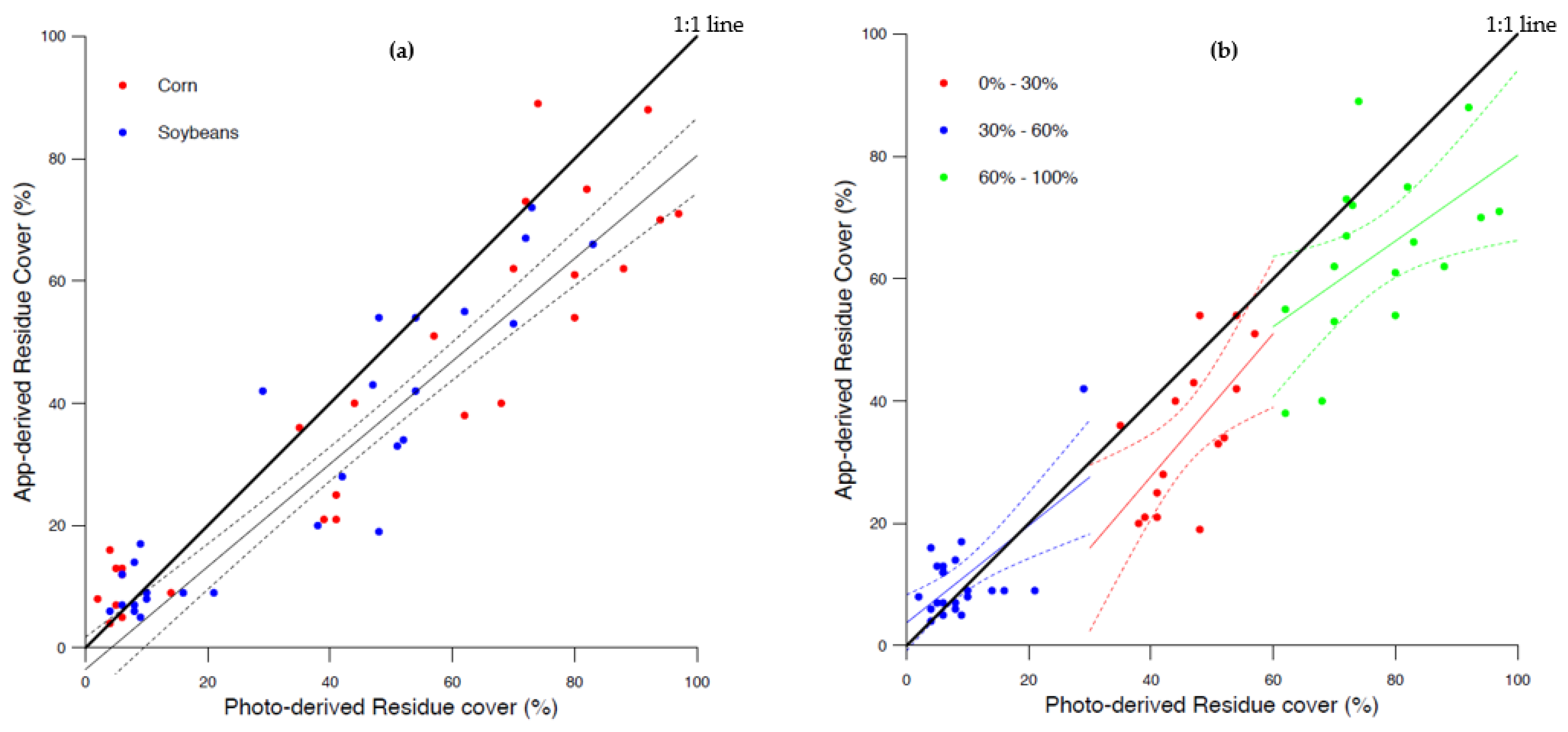
3.2. Relationship between Residue Cover Obtained by App vs. Photograph and Script Methods

Estimates of residue cover from each of the 54 photos were obtained from the app and compared to those obtained from photograph-grid and scripts methods. Analyses showed that percentage of residue cover estimates using the app method were strongly correlated to those estimated from photograph-grid (R² = 0.86; P < 0.001; n = 54;

Table 3. Summary statistics of relationships between residue cover percent as determined by app compared to photograph-grid and script methods in corn and soybean fields.

Residue	n	App vs. Photograph-Grid						App vs. Script
		R2	P	m	b	RMSE	Bias	R2	P	m	b	RMSE	Bias
All	54	0.86	0.00 *	0.77	2.84	13.3	−6.3	0.84	0.00 *	0.84	−3.45	15.4	−10.8
Corn	27	0.86	0.00 *	0.76	4.06	15.0	−7.4	0.86	0.00 *	0.84	−1.77	14.7	−9.6
Soybean	27	0.85	0.00 *	0.80	1.59	11.2	−5.3	0.79	0.00 *	0.81	−4.05	16.2	−12.0
Low	22	0.40	0.00 †	0.81	3.80	6.5	2.1	0.45	0.00 *	0.66	0.63	7.9	−4.6
Medium	15	0.40	0.00 ‡	1.18	−19.47	14.6	−11.2	0.13	0.17	0.47	9.81	21.8	−18.0
High	17	0.27	0.03 ‡	0.70	10.40	17.7	−13.0	0.43	0.00 †	1.25	−31.67	16.2	−12.3
≥30%	32	0.70	0.00 *	0.91	−6.73	16.4	−12.1	0.65	0.00 *	1.09	−20.8	19.0	−15.0

All data = all the sampled residue data were used (3 replicates per field; n = 54); LR = Low residue cover (CR + SB); MR = Medium residue cover (CR + SB); HR = High residue cover (CR + SB); ≤ 30% and > 30% represent plots with less and greater than 30% residue left on the field. n = total number of samples (measurements) used in the correlation. P-value <0.001 * and <0.01 †; the results is significant at P < 0.05. m is the slope of the line, and b is the y-intercept of the line. RMSE and Bias are expressed in percent (%).

and Figure 3a) and script methods (R² = 0.84; P < 0.001; n = 54; Table 3 and Figure 4a). When the three individual estimates per plot were averaged this correlation was even higher (photograph-grid: R² = 0.95, P < 0.001, n = 18; script: R² = 0.92, P < 0.001, n = 18; figures not shown here). With regards to estimation by residue type, corn showed higher R² than soybean for both photograph-grid (0.86 vs. 0.85) and script method (0.86 vs. 0.79) (Table 3; Figure 3b and Figure 4b). When the data were stratified by residue cover level (i.e., low, medium and high), the correlation between the app and photograph–grid was significant for low (R² = 0.40; P < 0.001; n = 22), medium (R² = 0.40; P < 0.05; n = 15) and high (R² = 0.27; P < 0.05; n = 17) residue estimates. As for the correlation between the app and script methods, only medium residue level was not significant (R² = 0.13, P <= 0.17, n = 15; Table 3). Fields with less than 30% residue cover (low) displayed statistically significant correlation and the lowest error (photograph-grid: R² = 0.40, RMSE = 6.5; script: R² = 0.45, RMSE = 7.9, respectively). Fields with more than 30%, residue, considered a conservation tillage practice, showed a higher correlation but also a higher error (photograph-grid: R² = 0.70, P < 0.001, RMSE = 16.4, script: R² = 0.65, P < 0.001, RMSE = 19.0, n = 32; Table 3).

The bias between the app measurements and both the photograph-grid and script methods were analyzed in this study (Table 3). For the photograph-grid method, the biases were generally under 10% for all the data (−6.3%) with a notable exception for fields with ≥30% residue covers (bias of −12.1%). For the script method, the biases were higher than those for the photograph-grid method (−10.8%) and under 15% overall (except for medium level residue; Table 3). Among all the significantly correlated residue estimates, fields with <30% residue cover showed the lowest biases (2.1% and −4.6%) and RMSE (6.5 and 7.9%) for both methods, respectively. This study also showed that soybean and corn residue covers have different trends in regard to the method used. Indeed, the bias of the app residue measurement compared to the photograph-grid method has higher for corn than soybean (−6.4% vs. −5.3%); whereas, corn residue measurements compared to the script method has lower bias than soybean (−9.6% vs. −12%). This finding (soybean residue cover has higher bias than corn) is consistent with other residue estimating studies in which errors were higher on soybeans compared to corn [20,21].

Finally, by dividing the field data between those with less than and greater than 30% residue cover, considered a conservation practice, results displayed the lowest (−4.1%) and highest (−15%) biases, respectively (data not shown in Table 3).

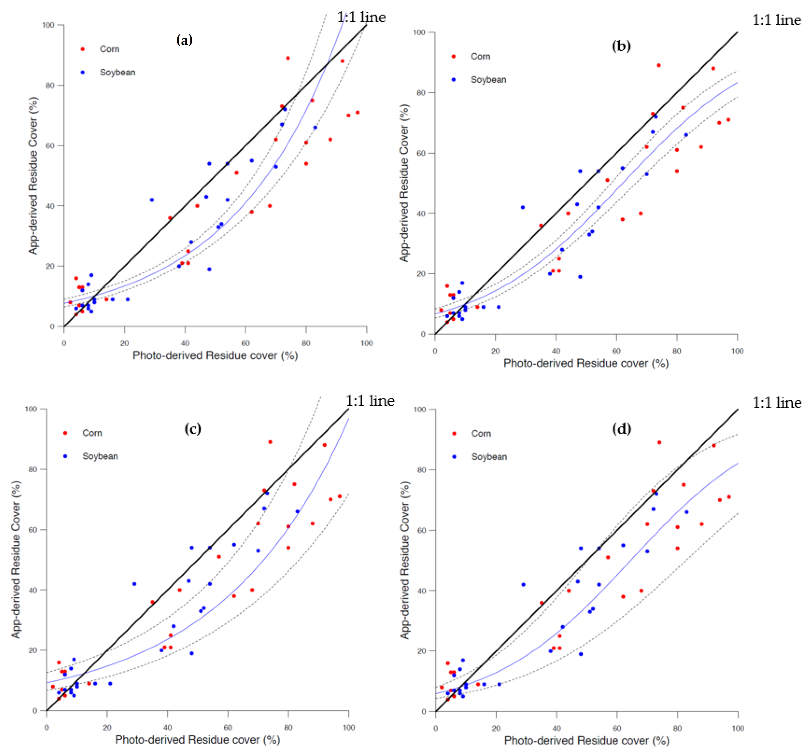
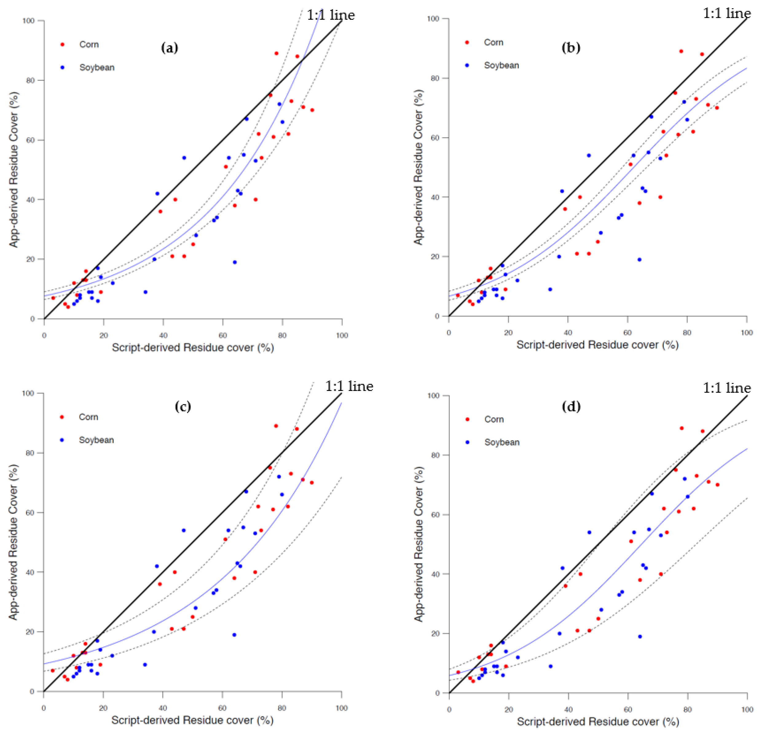
3.3. Exploring Non-Linear Relationship Alternative to Modelling the Residue Cover Data

Results of alternative distributions to model the data (app vs. photograph-grid and app vs. script) are summarized in Figure 5 and Figure 6 and

Table 4. Summary statistics of non-linear regression models between residue cover percent as determined by photograph-grid and script versus app methods.

Regression	App vs. Photograph-Grid				App vs. Script
	R2	P-Value	m (× 10−2)	b	R2	P-Value	m (× 10–2)	b
Log Transform	0.84	0.00 *	2.79	2.04	0.86	0.00 *	3.11	1.78
Logit Transform	0.86	0.00 *	4.24	−2.63	0.86	0.00 *	4.66	−3.00
Generalized Poisson	N/A	0.00 *	2.35	1.73	N/A	0.00 *	2.79	1.50
Beta	0.86 **	0.00 *	3.94	−2.43	0.86 **	0.00 *	4.29	−2.77

P-value: * <0.001. ** Pseudo R² refers to the squared correlation between the linear predictor for the mean and the link-transformed response [44]). N/A: Generalized Poisson models using R do not output a coefficient of determination or correlation coefficient.

. Exploratory analysis of the data was indicative of an exponential or logistic relationship between the app and script methods (Figure 5 and Figure 6). The relationship can be approximated using log and logit transformations of the response variable.

4. Discussion

Overall, this study has found that residue estimates from the FieldTRAKS app were in good agreement with those obtained with the photograph-grid method. There was a slight underestimation (–6.3%) and corn has a higher contribution to the bias than soybean, which could be explained by illumination phenomena. Analysis was done of freshly harvested fields in the fall and we believe that corn fields with high amounts of residue created a higher contrast between residue in shadow and illuminated areas in the same photograph, which leads to confusion for the app classifier. This can be supported by the fact that the high residue level has the highest RMSE and bias compared to low and medium classes (Table 3) and with most likely a higher contribution of corn plots (i.e., plot 9 in Table 1) to the bias. The results of this study suggest that the RMSE and bias are low for fields with <30% residue cover. This is particularly encouraging because these fields which are the ones most likely to need additional conservation practices, are more likely to be reliably assessed and identified using the app.

Similarly, the results indicate that residue estimates from the FieldTRAKS App were, overall, in good relative agreement (accuracy) with those obtained with the script method. Indeed, the app showed an underestimation of −10.8% relative to the script results. Contrary to the photograph-grid comparison, soybean showed a higher contribution to the bias than corn most likely because soybean residue pieces are relatively thinner than most corn pieces, increasing the likelihood to not be identified by the assessor. Second, there was a lower contrast between soil and soybean residue which lead to confusion for the app classifier. This study found that at high contrast or low contrast it is difficult for the app to adequately select training points to represent residue range, compared to grid count where forced to assess set points.

Exploratory analysis of the data was indicative of an exponential or logistic relationship between the app and script methods (Figure 5 and Figure 6). Inferences based on the standard errors reported using these ordinary least squares (OLS) regression estimates may be invalid and indeed seem too restrictive when 95% CI are considered. The data appear to be bimodal and/or under dispersed, meaning that the error terms are underestimated using OLS. It is recommended that a generalized Poisson or Beta regression be performed when modeling the variance of these data.

This study also found that residue cover estimated from the script method overestimates that obtained by the photograph-grid method although they are strongly correlated (Bias= 4.2%; RMSE = 7.5; R² = 0.96; regression results not shown). Difference in bias between these two methods could be attributed to the fact that grids used for grid point counting methods do not coincide and the script method, unlike the photograph-grid method, does not take into consideration the minimum residue size (i.e., to be counted, a piece of residue had to be ≥0.24 cm in diameter according to Shelton et al. [35]) as a rule of residue discrimination. Future iterations of the script method should require the implementation of this condition to be more comparable to field measurements.

Aside from reducing processing time and aiming to reduce effects from different users visually processing the photos, the script method is being developed to accumulate training and validation data sets for supervised and unsupervised statistical and machine learning approaches to residue estimation. The discrepancies and biases in the app vs. photo-grid and app vs. script methods, sampling error is a concern, as the reference counting method (photograph-grid and script) only sample a minute fraction of the millions of image pixels that the app classifies. The data appear to be bimodal and/or non-normally distributed, meaning that the error terms are underestimated using OLS. It is recommended that a generalized Poisson or Beta regression be performed when modeling the variance of these data. Even so, this study showed that the app can provide reliable and consistent measurements and that there is a potential for using apps (i.e., the FieldTRAKS Crop. Residue Estimator) to estimate residue over agricultural fields faster (i.e., each photo can be captured and classified in less than 3 min) provided the underestimation is corrected (i.e., by applying the regression equation).

There are many advantages of using the Crop Residue Estimator app. It could be employed: (i) to provide the farmers and crop advisors who manage the province’s cropland (i.e., corn, soybean and other grains) with the means to evaluate their crop residue cover easily; (ii) to provide farmers with convenient means of recording the results of the soil and water conservation practices applied on their farm (i.e., crop residue cover after harvest); (iii) to take advantage of mobile/communication technologies (i.e., tablets, smart phones) that are already purchased and used by landowners for other farm-related activities, such as collecting and organizing their field level operations; and (iv) to provide opportunities for farmers to demonstrate to government agencies and consumers their concern for soil and water conservation and their individual and collective on-farm efforts to improve environmental performance and sustainability of their land. These app-derived residue measurements could also be used for remote sensing data calibration and validation or for keeping track of the minimum recommended 30% soil cover throughout the year to reduce farmland topsoil and nutrient losses that impact water quality. Our future work will focus on exploring the use of app-derived residue estimates to determine whether very high resolution multi-spectral remote sensing datasets derived from Unmanned Aerial Vehicles (UAVs) could be used for future data collection efforts for high quality ground truth datasets of residue cover.

5. Conclusions

Mobile device remote sensing technologies and apps have attracted a great deal of interest from agricultural specialists, researchers and farmers in recent years. The interest in the use of these technologies in agriculture for deriving valuable information, measurements, or calculations has expanded rapidly over the last decade in conjunction with changes in technology as well as increase in computing and open-source image analysis software accessibility. There is no doubt that the use of apps among farmers will keep growing in the agricultural field and their use requires field testing and validation for different agriculture attributes. Therefore, studies aimed to evaluate apps’ potential usefulness in estimating agricultural residue percentage are of value. In this study, we assessed whether the analysis methods employed in the Crop Residue Estimator app developed by FieldTRAKS Solutions can be suitable for crop residue cover assessment and therefore, can provide a convenient and rapid measurement alternative to conventional methods (i.e., line-transect) which are considered laborious and time consuming. Overall, this study found that crop residue cover estimates obtained by the app showed a high correlation and an underestimation with those achieved by reference methods (photograph-grid and script methods). In comparison to the complexity of the photograph-grid or script method for residue counting, the app can easily obtain residue estimates on fields through a simple supervised classification process using 4–8 representative training points from the image. Finally, this study showed that mobile devices equipped with apps can perform adequate digital crop residue analysis particularly for lower residue amounts (<30% residue cover) below the threshold considered a conservation practice. However, for remote sensing studies where more accurate measurements of residue are necessary for providing ground-based corroboration datasets, the photograph-grid or the script based approach are recommended.

References

1. Daughtry, C.S.T.; Hunt, E.R., Jr. Mitigating the effects of soil and residue water contents on remotely sensed estimates of crop residue cover. Remote Sens. Environ. 2008, 112, 1647–1657. [Google Scholar] [CrossRef]
2. Kumar, K.; Goh, K.M. Crop residues and management practices: Effects on soil quality, soil nitrogen dynamics, crop yield and nitrogen recovery. Adv. Agron. 1999, 68, 197–319. [Google Scholar]
3. Mailapalli, D.R.; Burger, M.; Horwath, W.R.; Wallender, W.W. Crop residue biomass effects on agricultural runoff. Appl. Environ. Soil Sci. 2013, 2013, 805206. [Google Scholar] [CrossRef]
4. Enciso, J.; Nelson, S.D.; Perea, H.; Uddameri, V.; Kannan, N.; Gregory, A. Impact of residue management and subsurface drainage on non-point source pollution in the Arroyo Colorado. Sustain. Water Qual. Ecol. 2014, 3–4, 25–32. [Google Scholar] [CrossRef]
5. Aguilar, J.; Evans, R.; Daughtry, C.S.T. Performance assessment of the cellulose absorption index method for estimating crop residue cover. J. Soil Water Conserv. 2012, 67, 202–210. [Google Scholar] [CrossRef]
6. Molder, B.; Cockburn, J.; Berg, A.; Lindsay, J.; Woodrow, K. Sediment-assisted nutrient transfer from a small, no-till, tile drained watershed in Southwestern Ontario, Canada. Agric. Water Manag. 2015, 152, 31–40. [Google Scholar] [CrossRef]
7. Shelton, D.P.; Dickey, E.C.; Jasa, P.J.; Kanable, R.; Smydra Krotz, S. Using the Line-Transect Method to Estimate Percent Residue Cover. Biol. Syst. Eng. 1990, G-20. Available online: https://digitalcommons.unl.edu/biosysengfacpub/289/ (accessed on 21 February 2018).
8. Huggins, D.R.; Reganold, J.P. No-till: The quiet revolution. Sci. Am. 2008, 299, 70–77. [Google Scholar] [CrossRef] [PubMed]
9. Lal, R. Sequestering carbon and increasing productivity by conservation agriculture. J. Soil Water Conserv. 2015, 70, 55A–62A. [Google Scholar] [CrossRef]
10. OMAFRA. Great Lakes Agricultural Stewardship: Helping Ontario Farmers Keep the Great Lakes Healthy. 2015. Available online: https://news.ontario.ca/omafra/en/2015/02/great-lakes-agriculturalstewardship.html (accessed on 21 February 2018).
11. Clarke, N.D.; Stone, J.A.; Vyn, T.J. Conservation tillage expert system for southwestern Ontario: Multiple experts and decision techniques. AI Appl. Nat. Resour. Manag. 1990, 4, 78–84. [Google Scholar]
12. Patni, N.K.; Masse, L.; Jui, P.Y. Groundwater quality under conventional and no-tillage: I. Nitrate, electrical conductivity and pH. J. Environ. Qual. 1998, 27, 869–877. [Google Scholar] [CrossRef]
13. Yang, W.; Sheng, C.; Voroney, P. Spatial targeting of conservation tillage to improve water quality and carbon retention benefits. Can. J. Agric. Econ. 2005, 53, 477–500. [Google Scholar] [CrossRef]
14. Kochsiek, A.E.; Knops, J.M.H.; Brassil, C.E.; Arkebauer, T.J. Maize and soybean litter-carbon pool dynamics in three no-till systems. Soil Sci. Soc. Am. J. 2013, 77, 226–236. [Google Scholar] [CrossRef]
15. Congreves, K.A.; Smith, J.M.; Németh, D.D.; Hooker, D.C.; Van Eerd, L.L. Soil organic carbon and land use: Processes and potential in Ontario’s long-term agro-ecosystem research sites. Can. J. Soil Sci. 2014, 94, 317–336. [Google Scholar] [CrossRef]
16. Van Eerd, L.L.; Congreves, K.A.; Hayes, A.; Verhallen, A.; Hooker, D.C. Long-term tillage and crop rotation effects on soil quality, organic carbon and total nitrogen. Can. J. Soil Sci. 2014, 94, 303–315. [Google Scholar] [CrossRef]
17. Smith, P.; Martino, D.; Cai, Z.; Gwary, D.; Janzen, H.; Kumar, P.; McCarl, B.; Ogle, S.; O’Mara, F.; Rice, C.; et al. Greenhouse gas mitigation in agriculture. Philos. Trans. R. Soc. 2008, 363, 789–813. [Google Scholar] [CrossRef] [PubMed]
18. Ketcheson, J.W.; Stonehouse, D.P. Conservation tillage in Ontario. J. Soil Water Conserv. 1983, 38, 253–254. [Google Scholar]
19. Dodd, V.A.; Grace, P.M.; Dickey, E.C.; Shelton, D.P.; Meyer, G.E.; Fairbanks, K.T. Determining crop residue cover with electronic image analysis. Biol. Syst. Eng. 1989, 3057–3063. Available online: https://digitalcommons.unl.edu/biosysengfacpub/238/ (accessed on 21 February 2018).
20. Laamrani, A.; Joosse, P.; Feisthauer, N. Determining the number of measurements required to estimate crop residue cover by different methods. Soil Water Conserv. 2017, 72, 471–479. [Google Scholar] [CrossRef]
21. Pacheco, A.; McNairn, H. Evaluating multispectral remote sensing and spectral unmixing analysis for crop residue mapping. Remote Sens. Environ. 2010, 114, 2219–2228. [Google Scholar] [CrossRef]
22. Dehnen-Schmutz, K.; Foster, G.L.; Owen, L.; Persello, S. Exploring the role of smartphone technology for citizen science in agriculture. Agron. Sustain. Dev. 2016, 36, 1–9. [Google Scholar] [CrossRef]
23. Statistics Canada. Table 004-0243—Census of Agriculture, Farms Reporting Technologies in the Year Prior to the Census. 2016. Available online: http://www5.statcan.gc.ca/cansim/a26?lang=eng&retrLang=eng&id=0040243&tabMode=dataTable&p1=-1&p2=11&srchLan=-1 (accessed on 22 February 2018).
24. Booth, T.D.; Cox, S.E.; Berryman, R.D. Point sampling digital imagery with “SamplePoint”. Environ. Monit. Assess. 2006, 123, 97–108. [Google Scholar] [CrossRef] [PubMed]
25. Lynch, T.M.H.; Barth, S.; Dix, P.J.; Grogan, D.; Grant, J.; Grant, O.M. Ground Cover Assessment of Perennial Ryegrass Using Digital Imaging. Agron. J. 2015, 107, 2347–2352. [Google Scholar] [CrossRef]
26. Patrignani, A.; Ochsner, T.E. Canopeo: A Powerful New Tool for Measuring Fractional Green Canopy Cover. Agron. J. 2015, 107, 312–2320. [Google Scholar] [CrossRef]
27. Karcher, D.E.; Richardson, M.D. Batch Analysis of Digital Images to Evaluate Turfgrass Characteristics. Crop Sci. 2005, 45, 1536–1539. [Google Scholar] [CrossRef]
28. Confalonieri, R.; Foi, M.; Casa, R.; Aquaro, S.; Tona, E.; Peterle, M.; Boldini, A.; De Carli, G.; Ferrari, A.; Finotto, G.; et al. Development of an app for estimating leaf area index using a smartphone. Trueness and precision determination and comparison with other indirect methods. Field Crops Res. 2013, 96, 67–74. Available online: http://dx.doi.org/10.1016/j.compag.2013.04.019 (accessed on 21 February 2018). [CrossRef]
29. Campos-Taberner, M.; Garcia-Haro, F.; Moreno, A.; Gilabert, M.; Sanchez-Ruiz, S.; Martinez, B.; Camps-Valls, G. Mapping leaf area index with a smartphone and Gaussian processes. IEEE Geosci. Remote Sens. Lett. 2015, 12, 2501–2505. [Google Scholar] [CrossRef]
30. Vesali, F.; Omid, M.; Mobli, H.; Kaleita, A. Feasibility of using smart phones to estimate chlorophyll content in corn plants. Photosynthetica 2017, 55, 603–610. [Google Scholar] [CrossRef]
31. Salk, C.F.; Sturn, T.; See, L.; Fritz, S.; Perger, C. Assessing quality of volunteer crowdsourcing contributions: Lessons from the Cropland Capture game. Int. J. Digit. Earth 2016, 9, 410–426. [Google Scholar] [CrossRef] [Green Version]
32. Molinier, M.; López-Sánchez, C.A.; Toivanen, T.; Korpela, I.; Corral-Rivas, J.J.; Tergujeff, R.; Häme, T. Relasphone-Mobile and Participative In Situ Forest Biomass Measurements Supporting Satellite Image Mapping. Remote Sens. 2016, 8, 869. [Google Scholar] [CrossRef]
33. FieldTRAKS Solutions. © FieldTRAKS Solutions 2004–2016. Available online: http://www.fieldtraks.ca/ (accessed on 15 January 2018).
34. Kludze, H.; Deen, B.; Dutta, A. Report on Literature Review of Agronomic Practices for Energy Crop Production under Ontario Conditions. 2011, pp. 494–504. Available online: https://ofa.on.ca/uploads/userfiles/files/u%20of%20g%20ofa%20project-final%20report%20july%2004-2011%20 (accessed on 15 January 2018).
35. Kludze, H.; Deen, B.; Weersink, A.; van Acker, R.; Janovicek, K.; De Laporte, A.; McDonald, A. Estimating sustainable crop residue removal rates and costs based on soil organic matter dynamics and rotational complexity. Biomass Bioenergy 2013, 56, 607–618. [Google Scholar] [CrossRef]
36. Rasmussen, J.; Norremark, M.; Bibby, B.M. Assessment of leaf cover and crop soil cover in weed harrowing research using digital images. Weed Res. 2007, 47, 299–310. [Google Scholar] [CrossRef]
37. Shelton, D.P.; Kanable, R.; Jasa, P.J. Estimating Percent Residue Cover Using the Line-Transect Method. Bol. Syst. Eng. 1993. Available online: digitalcommons.unl.edu/cgi/viewcontent.cgi?article=1255&context=biosysengfacpub (accessed on 21 February 2018).
38. R Development Core Team. A Language and Environment for Statistical Computing. 2011. Available online: http://www.R-project.org/ (accessed on 15 January 2018).
39. Hilbe, J.M. Modeling Count Data; Cambridge University Press: New York, NY, USA, 2014; Chapter 9. [Google Scholar]
40. Singh, K.P.; Famoye, F. Analysis of Rates Using a Generalized Poisson Regression Model. Biom J. 1993, 35, 917–923. [Google Scholar] [CrossRef]
41. Smithson, M.; Verkuilen, J. A Better Lemon Squeezer? Maximum-Likelihood Regression with Beta-Distributed Dependent Variables. Psychol. Methods 2006, 11, 54–71. [Google Scholar] [CrossRef] [PubMed]
42. Cribari-neto, F.; Zeileis, A. Beta Regression in R. J. Stat. Softw. 2010, 34, 1–24. [Google Scholar] [CrossRef]
43. Ryu, D.; Famiglietti, J.S. Characterization of footprint-scale surface soil moisture variability using Gaussian and beta distribution functions during the Southern Great Plains 1997 (SGP97) hydrology experiment. Water Resour. Res. 2005, 41, 1–13. [Google Scholar] [CrossRef]
44. Ferrari, S.; Cribari-neto, F.; Ferrari, S.L.P.; Cribari-neto, F. Beta Regression for Modelling Rates and Proportions. J. Appl. Stat. 2004, 31, 799–815. [Google Scholar] [CrossRef]
Figure 1. Study area within the Lake Erie watershed, southern Ontario, Canada. The 18 plots used in this study were located south of the city of London.
Sensors 18 00708 g001
Figure 2. Examples of vertical photographs taken over soybean (a) and corn (c) fields. The photograph-grid method used superimposed, uniformly spaced 10 by 10 digital grid intersections (b). The app estimated crop residue is displayed in (d) as a thematic classified map using a two-color palette legend (residue class in red vs. no-residue class in gray. (c,d) show an example of the app method input and output. This example shows an evident underestimation of the app-derived crop residue compared to that from the photograph-grid method (i.e., 62% vs. 88%, respectively).
Sensors 18 00708 g002
Figure 3. Relationships between residue cover percent as determined by photograph-grid and app: (a) residue cover (corn = red dots and soybean = blue dots); and (b) residue levels (Low = blue, medium= red and high = green). Related statistics are shown in Table 2.
Sensors 18 00708 g003
Figure 4. Relationships between residue cover percent as determined by script and app: (a) residue cover (corn = red dots and soybean = blue dots); and (b) residue levels (Low < 30%, medium= 30–60% and high > 60%). Related statistics (i.e., R2) are shown in Table 3.
Sensors 18 00708 g004
Figure 5. Relationships between residue cover percent as determined by photograph-grid and app with 95% CI: (a) OLS log-linear regression; (b) OLS logit-linear regression, (c) generalized Poisson regression; (d) Beta regression with logit link.
Sensors 18 00708 g005
Figure 6. Relationships between residue cover percent as determined by script and app with 95% CI: (a) OLS log-linear regression; (b) OLS logit-linear regression; (c) generalized Poisson regression; (d) Beta regression with logit link.
Sensors 18 00708 g006