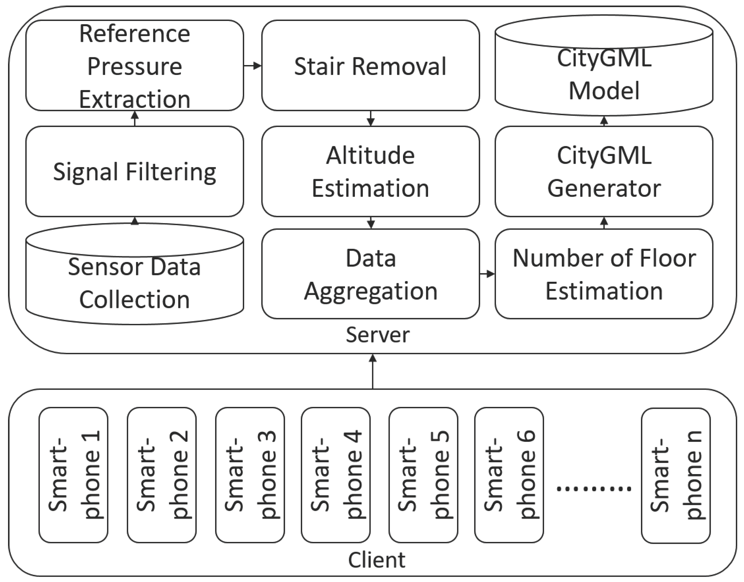
Figure 1.
The overall architecture of our system [
15].
Figure 1.
The overall architecture of our system [
15].
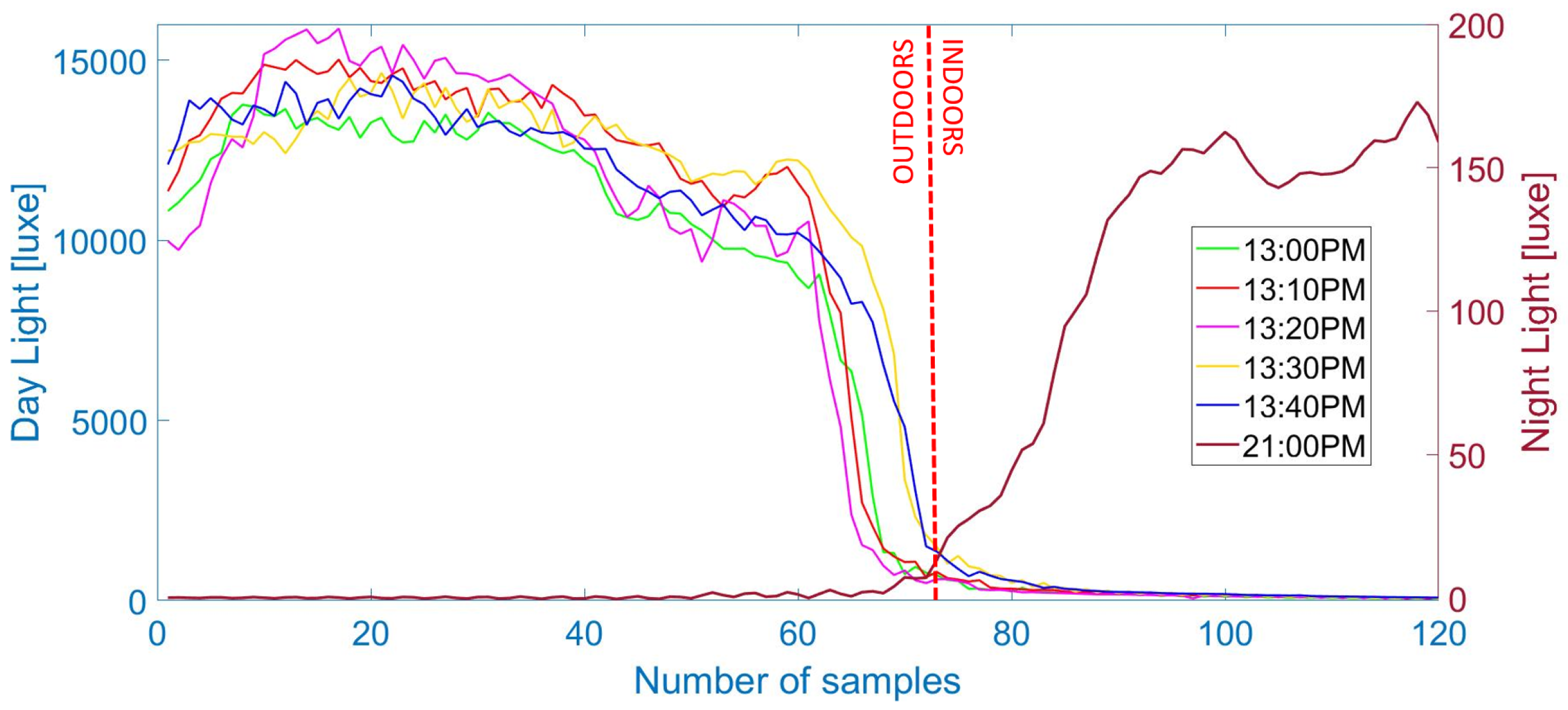
Figure 2.
Light data from six outdoor–indoor transitions (OITransitions) collected during the same day, five during day time and one during night. As can be seen, during the OITransition (after the 70th sample), the light intensity rapidly decreases during the day (left axis) and increases during the night (right axis).
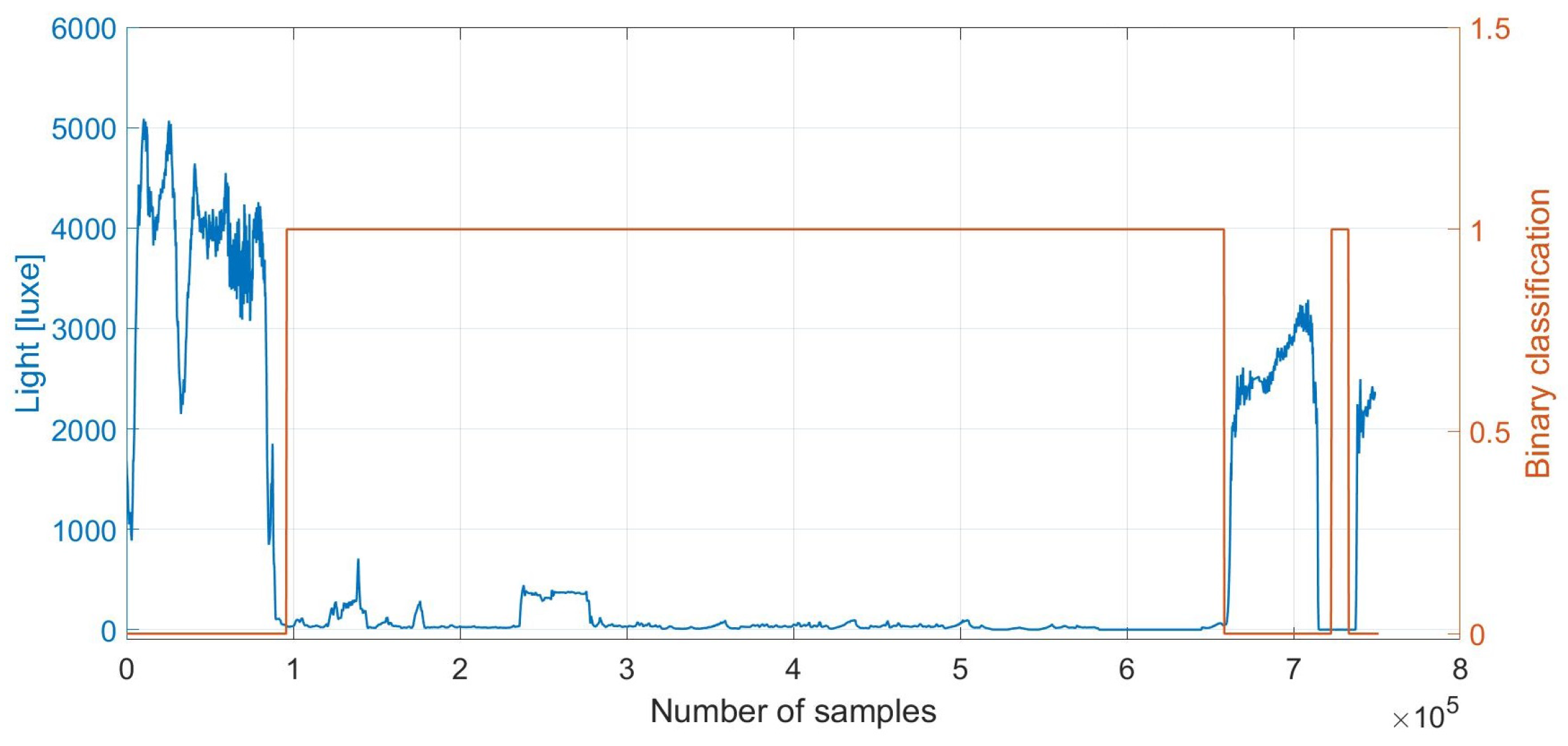
Figure 3.
Outdoor–indoor transition (OITransition) classification using light. The binary flag of 1 (orange line and right axis) indicates indoor area. We note that during the period after sample , the smartphone was in a pocket. However, it is wrongly classified as indoors. This demonstrates the need for fusion with the proximity sensor, which can indicate whether the phone is exposed (the light sensor can be trusted) or not.
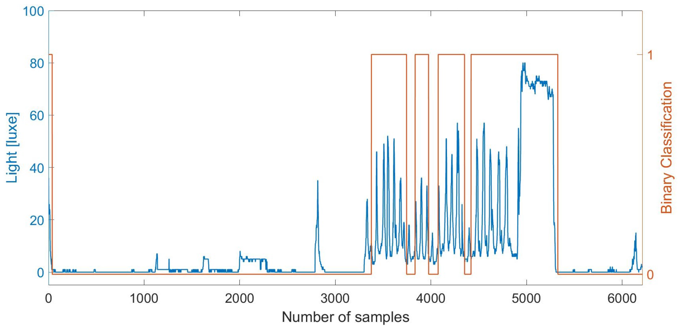
Figure 4.
Outdoor–indoor transition (OITransition) classification using light at night. The binary flag of 1 (orange line and right axis) indicates indoor area.
Figure 4.
Outdoor–indoor transition (OITransition) classification using light at night. The binary flag of 1 (orange line and right axis) indicates indoor area.
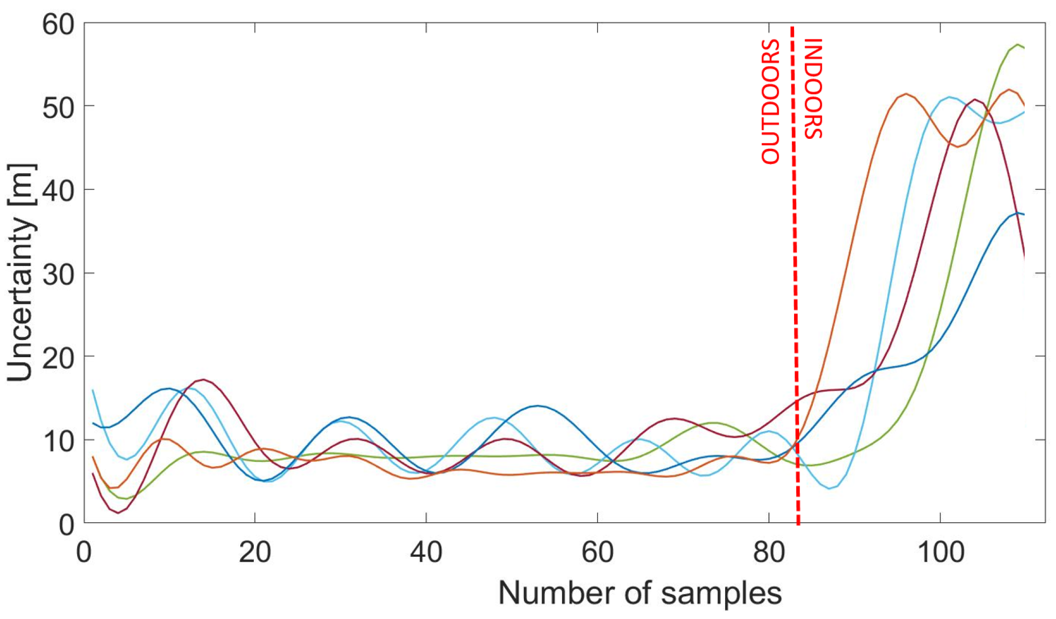
Figure 5.
GPS uncertainty data from five outdoor–indoor transitions (OITransitions). As can be seen, at the moment of the transition after the 100th sample, the uncertainty rapidly increased.
Figure 5.
GPS uncertainty data from five outdoor–indoor transitions (OITransitions). As can be seen, at the moment of the transition after the 100th sample, the uncertainty rapidly increased.
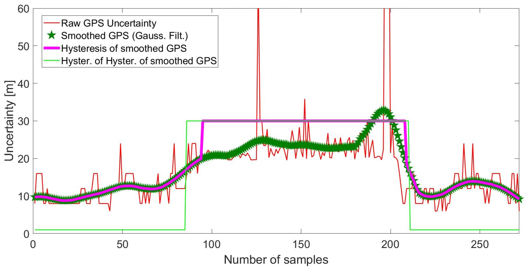
Figure 6.
Smoothing and hysteresis thresholding of raw GPS uncertainty signal.
Figure 6.
Smoothing and hysteresis thresholding of raw GPS uncertainty signal.
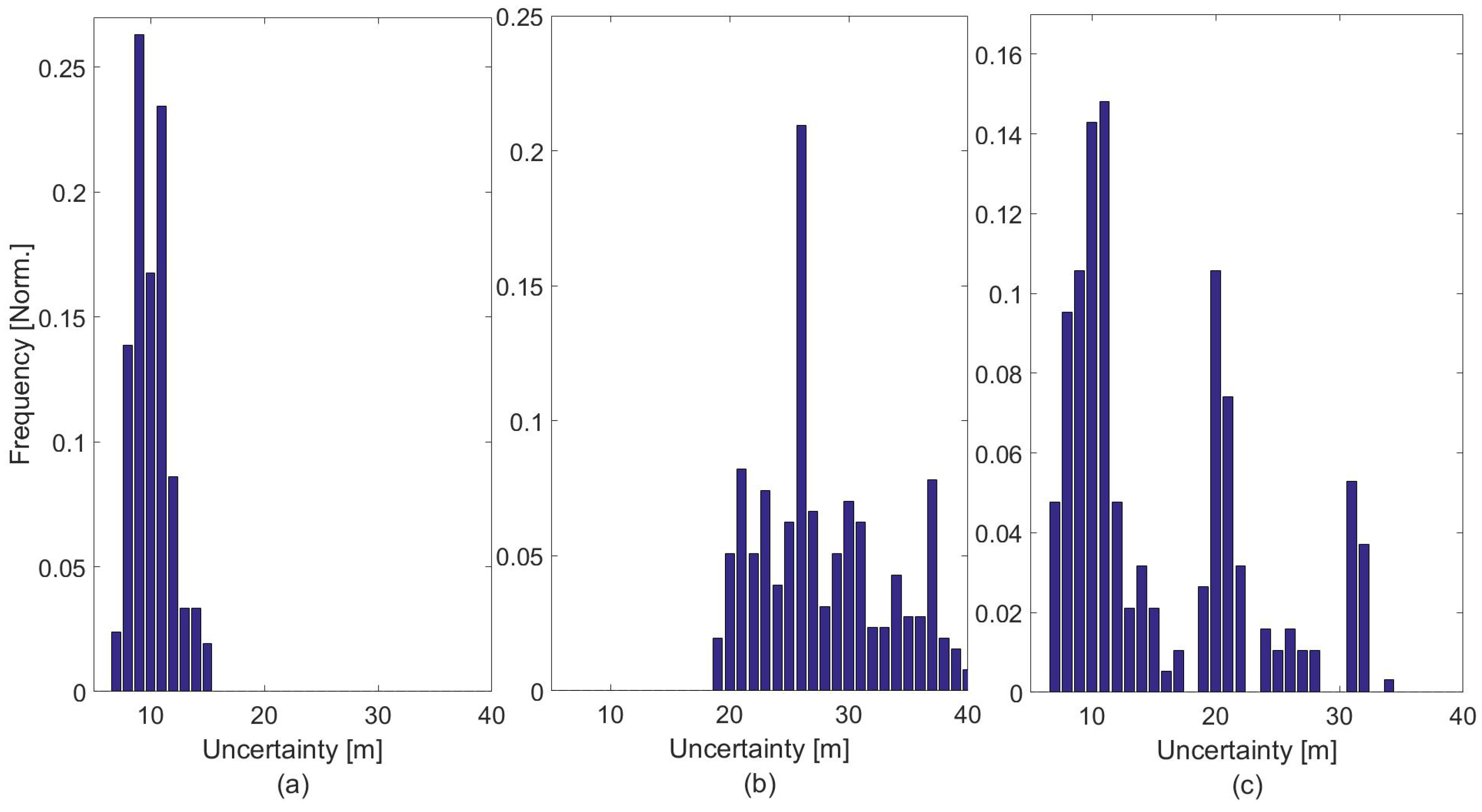
Figure 7.
Frequency of GPS uncertainty from data collected from outdoors (a), indoors (b) and during an OITransition.
Figure 7.
Frequency of GPS uncertainty from data collected from outdoors (a), indoors (b) and during an OITransition.
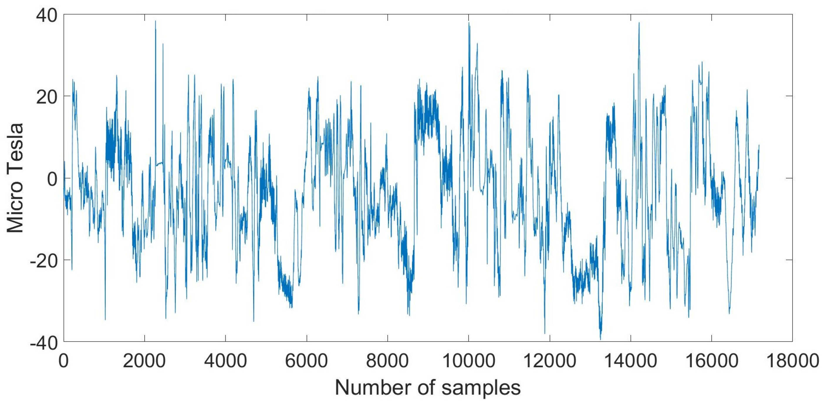
Figure 8.
Magnetometer signal from walking into four consecutive buildings.
Figure 8.
Magnetometer signal from walking into four consecutive buildings.
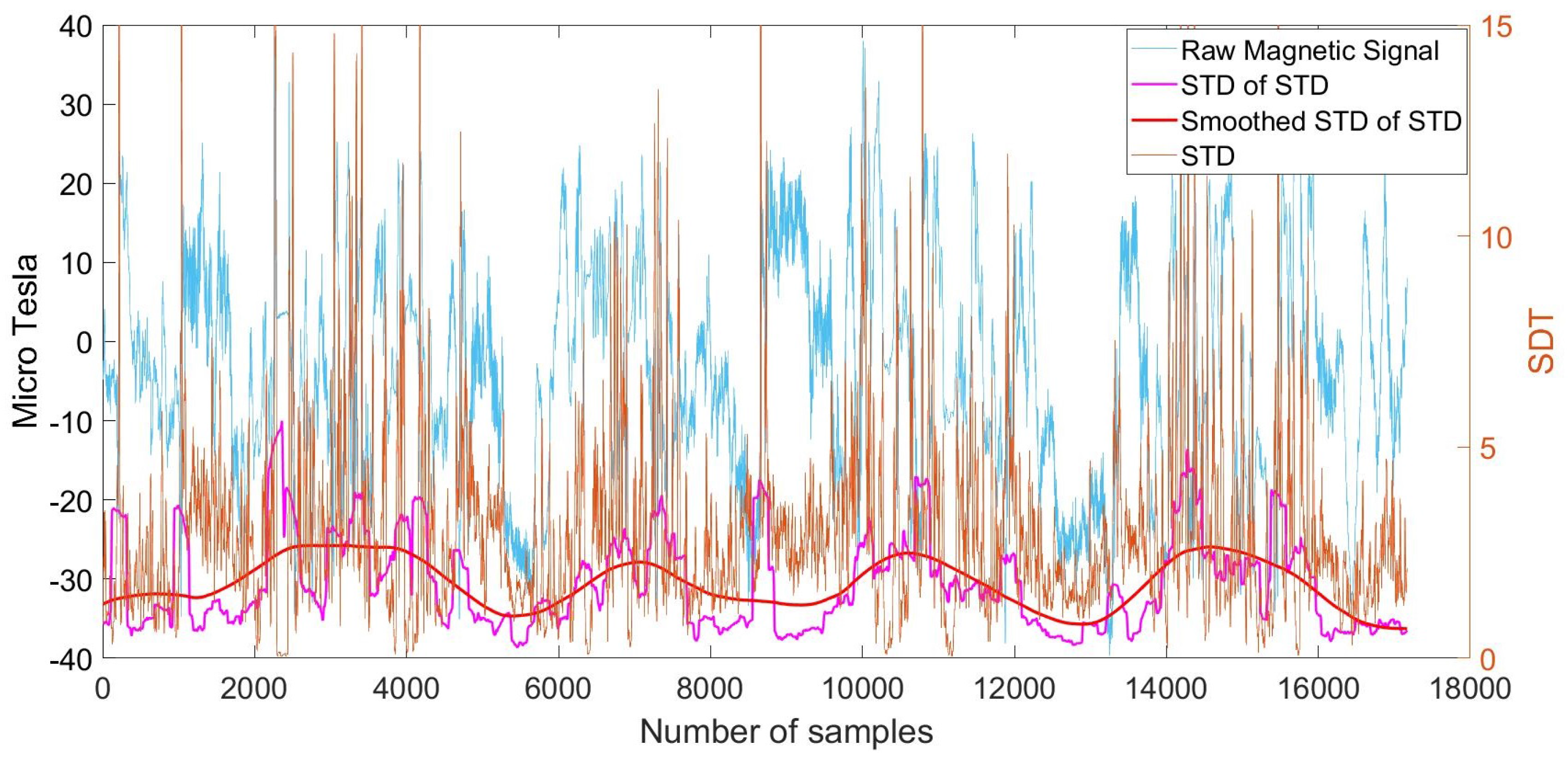
Figure 9.
Magnetometer signal from walking into four consecutive buildings and corresponding smoothed moving Standard Deviation (STD) of moving STD with kernel size of 500.
Figure 9.
Magnetometer signal from walking into four consecutive buildings and corresponding smoothed moving Standard Deviation (STD) of moving STD with kernel size of 500.
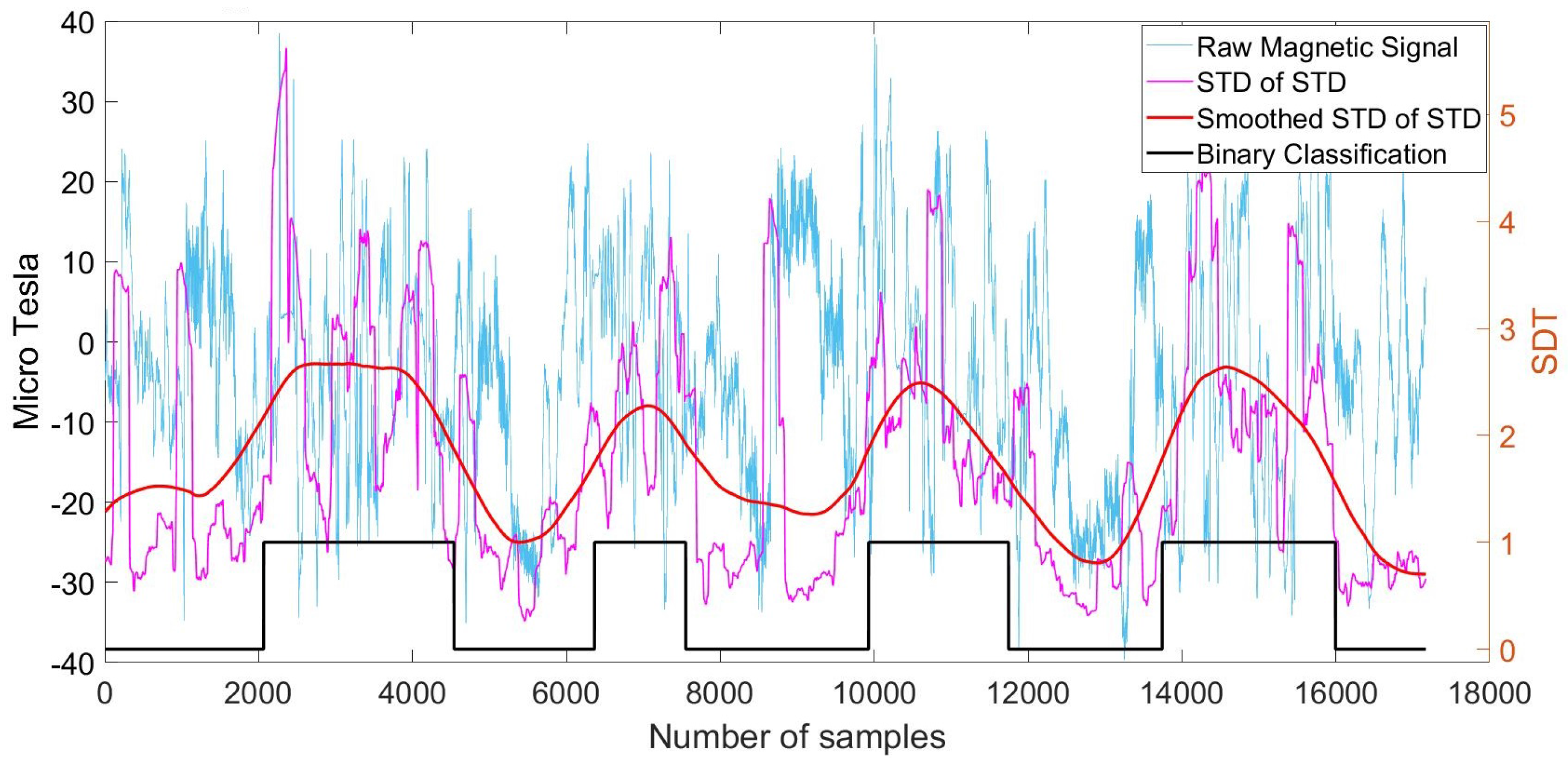
Figure 10.
Magnetometer signal from walking into four consecutive buildings and corresponding smoothed moving STD of the disturbance, with kernel size of 200 samples, and the final binary classification.
Figure 10.
Magnetometer signal from walking into four consecutive buildings and corresponding smoothed moving STD of the disturbance, with kernel size of 200 samples, and the final binary classification.
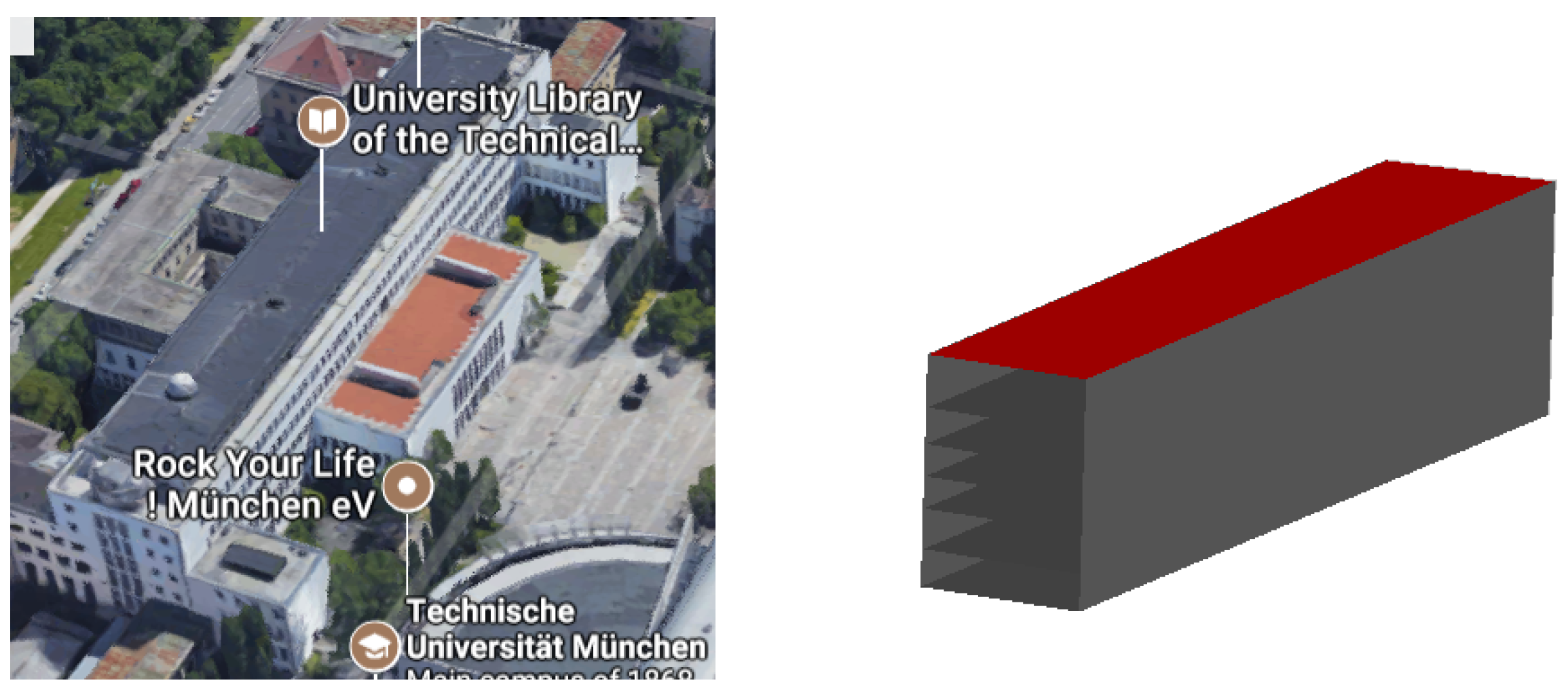
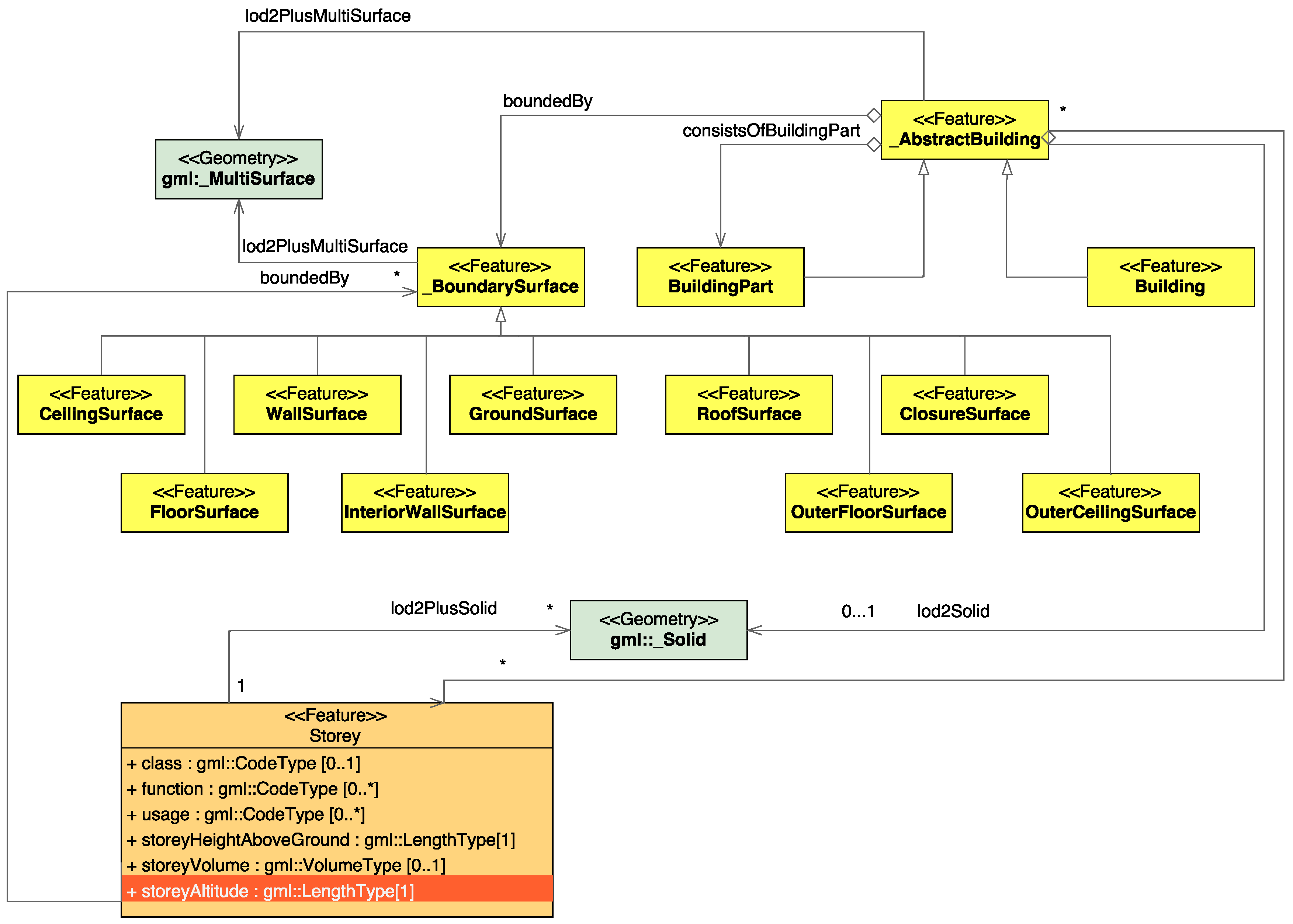
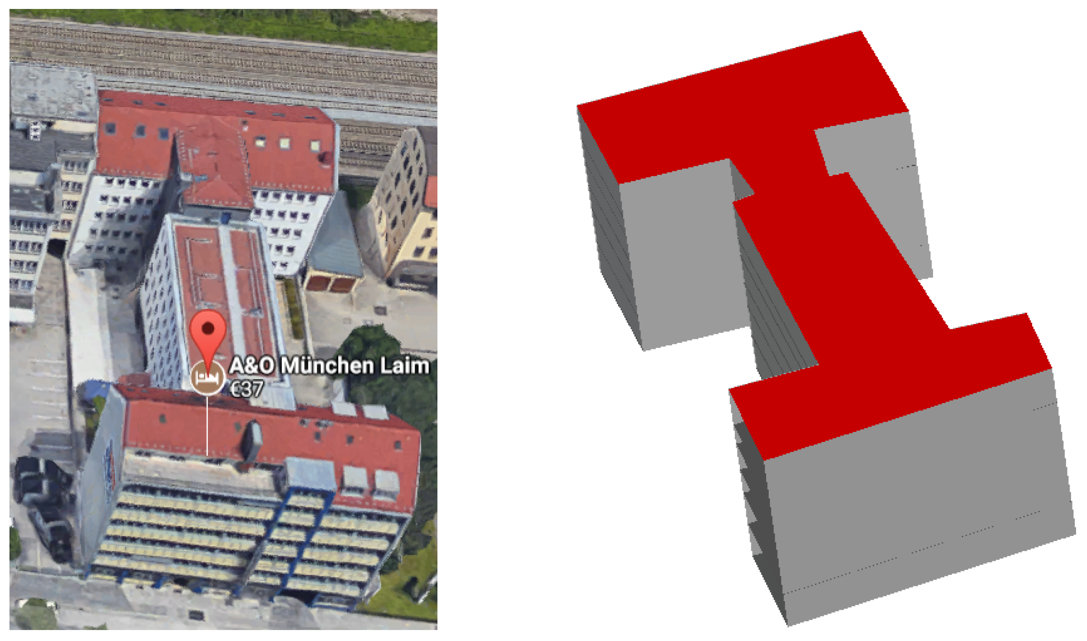
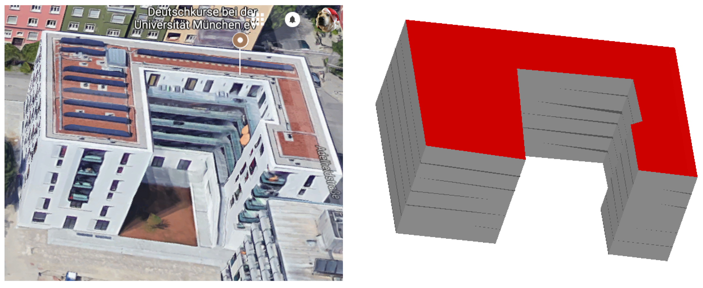
Figure 11.
The proposed level of detail two plus (LoD2+) model, which carries information about the number of stores as proposed by [
11] and their corresponding altitudes.
Figure 11.
The proposed level of detail two plus (LoD2+) model, which carries information about the number of stores as proposed by [
11] and their corresponding altitudes.
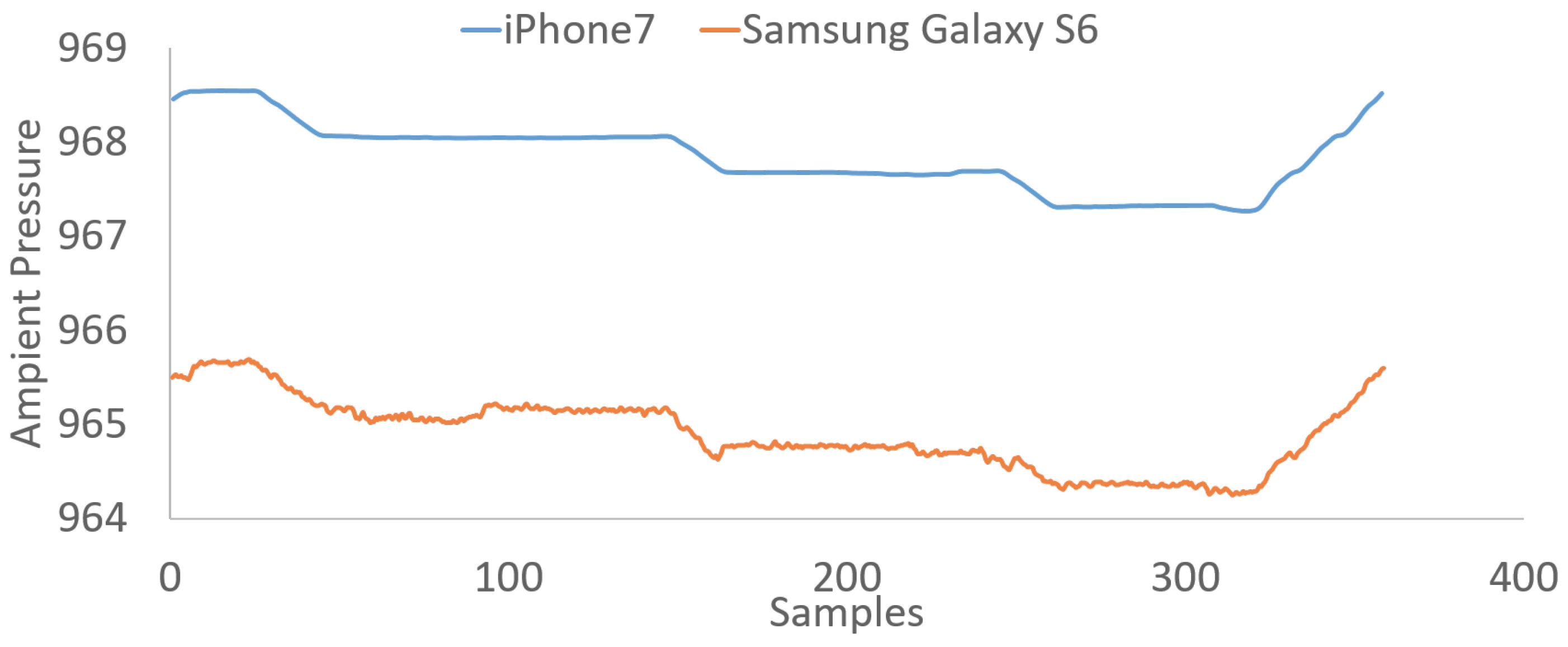
Figure 12.
Data collected from an iPhone 7 and a Samsung Galaxy S6, while the user had climbed three floors upwards and the same number of floors downwards.
Figure 12.
Data collected from an iPhone 7 and a Samsung Galaxy S6, while the user had climbed three floors upwards and the same number of floors downwards.
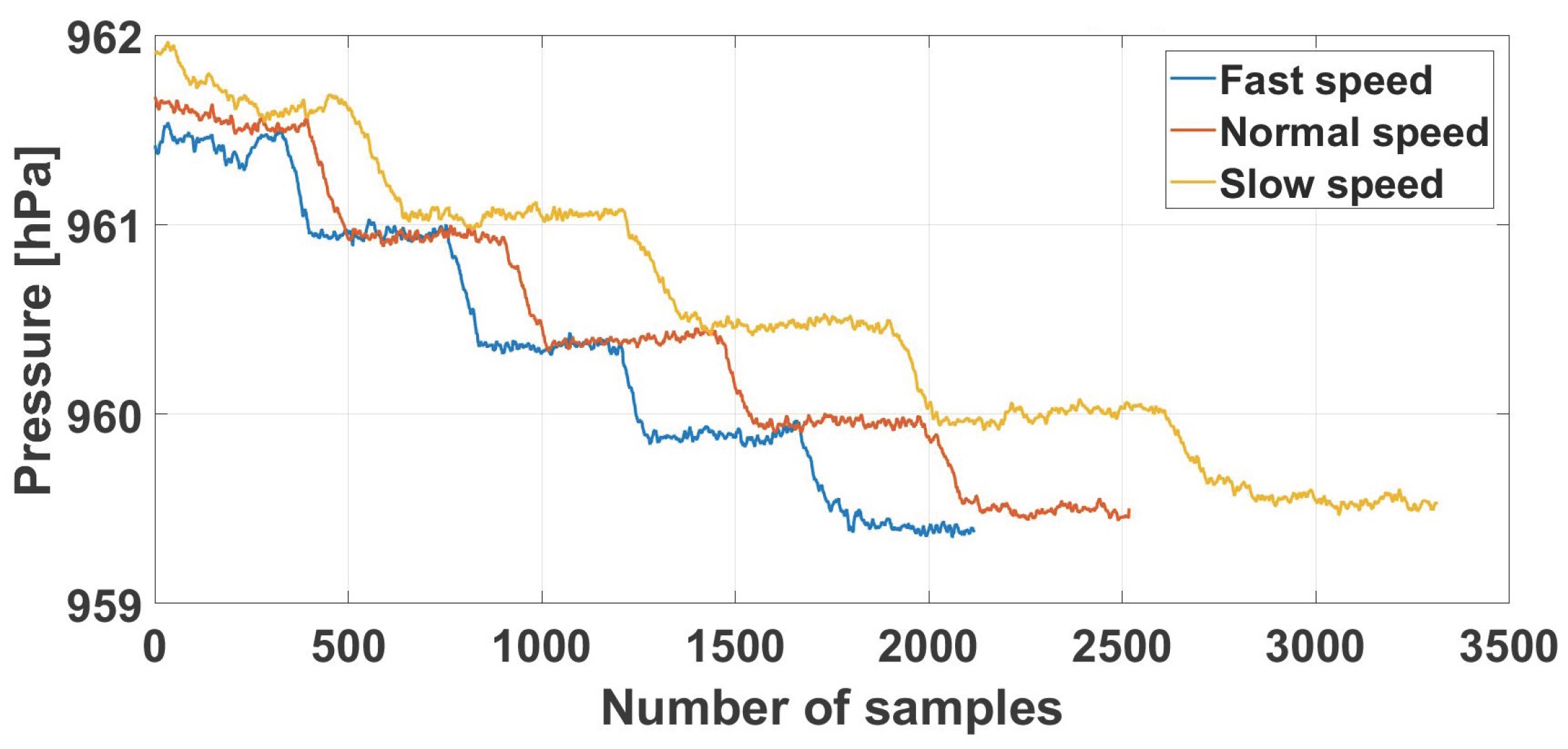
Figure 13.
Dataset used for the evaluation of the stair removal method. The data was collected from the same route for three different visits and walking velocities, approximately 1×, 1.5× and 2× [
15].
Figure 13.
Dataset used for the evaluation of the stair removal method. The data was collected from the same route for three different visits and walking velocities, approximately 1×, 1.5× and 2× [
15].
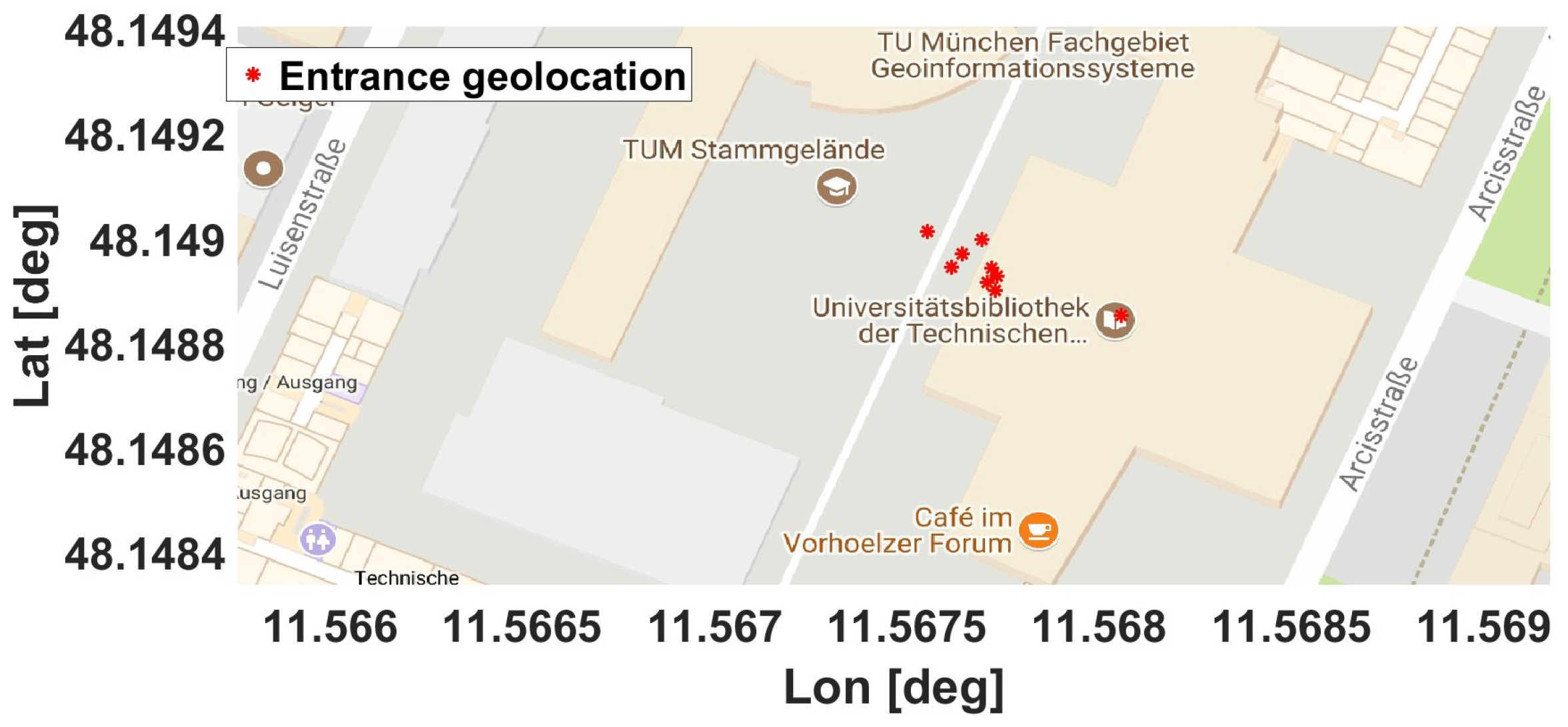
Figure 14.
Locations that correspond to the detection of the outdoor–indoor transition (OITransition). The figure includes nine different determined locations for the entrance to the building (red dots) [
15].
Figure 14.
Locations that correspond to the detection of the outdoor–indoor transition (OITransition). The figure includes nine different determined locations for the entrance to the building (red dots) [
15].
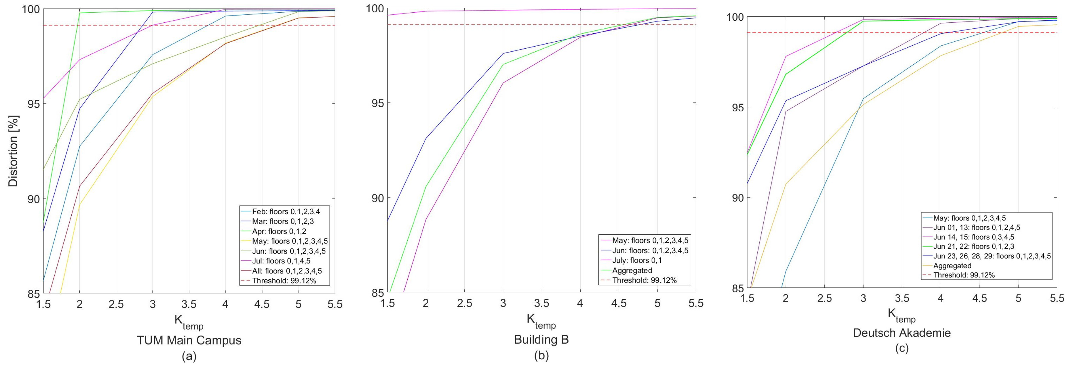
Figure 15.
Elbow method result for three test buildings (a) TUM Main Campus, (b) Building B, (c) Deutsche Akademie.
Figure 15.
Elbow method result for three test buildings (a) TUM Main Campus, (b) Building B, (c) Deutsche Akademie.
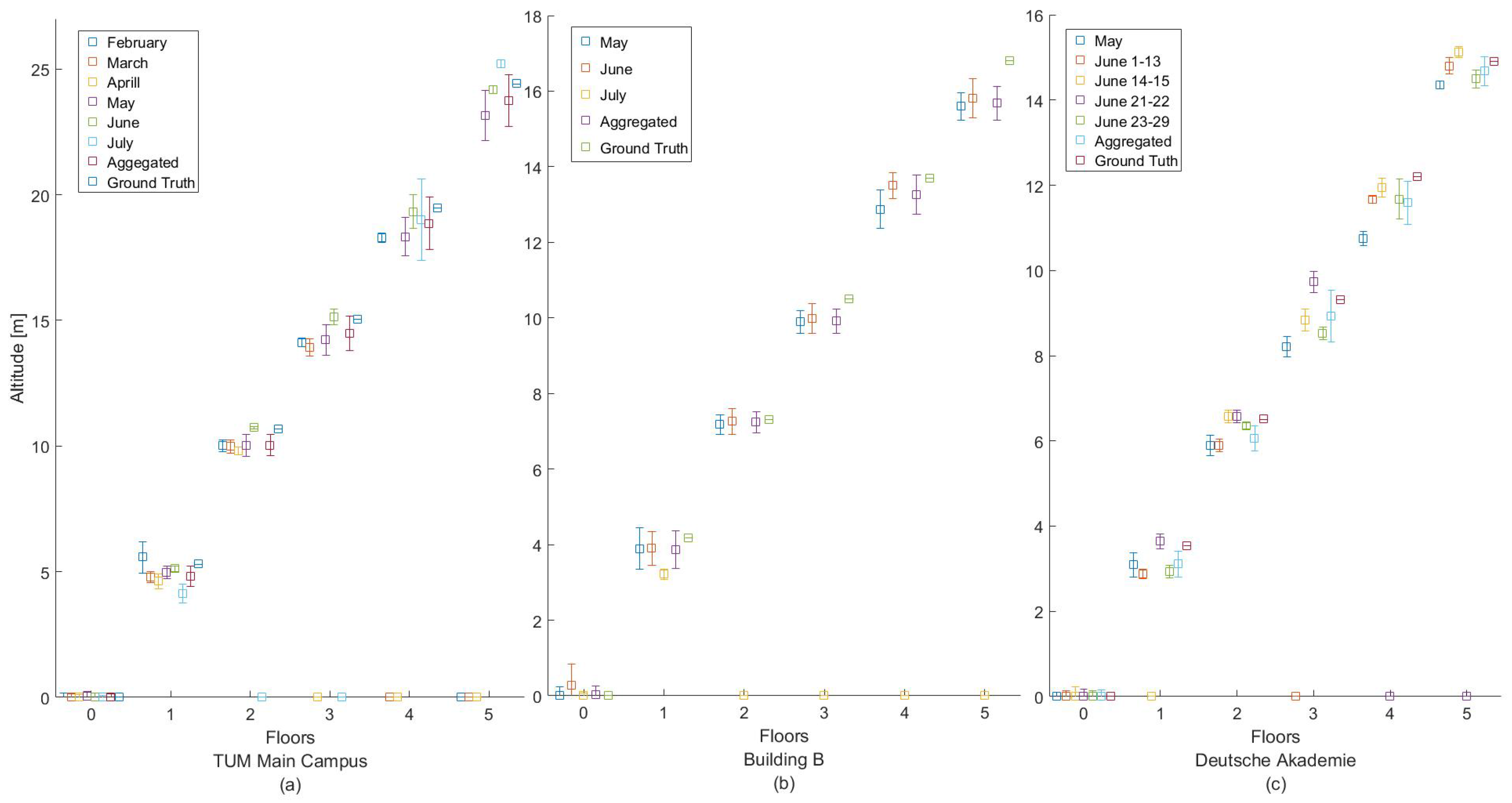
Figure 16.
Estimated altitude and ground truth for each floor height for three test buildings (a) TUM Main Campus, (b) Building B, (c) Deutsche Akademie.
Figure 16.
Estimated altitude and ground truth for each floor height for three test buildings (a) TUM Main Campus, (b) Building B, (c) Deutsche Akademie.
Table 1.
Fusion Rules.
| Proximity | Light | GPS | Magnetic | Indoor | Outdoor | Fusion Model |
|---|
| False | 0 | 0 | 0 | F | T | Voting |
| False | 0 | 0 | 1 | F | T | Voting |
| False | 0 | 1 | 0 | F | T | Voting |
| False | 0 | 1 | 1 | T | F | Voting |
| False | 1 | 0 | 0 | F | T | Voting |
| False | 1 | 0 | 1 | T | F | Voting |
| False | 1 | 1 | 0 | T | F | Voting |
| False | 1 | 1 | 1 | T | F | Voting |
| True | — | 0 | 0 | F | T | |
| True | — | 0 | 1 | F | T | |
| True | — | 1 | 0 | F | T | |
| True | — | 1 | 1 | T | F | |
Table 2.
Collected Data used for evaluation. The table shows the date of collecting the data, the time, the indicated temperature from AccuWeather (T A) and Google (T A) (unit: °C), the relative humidity from the same two sources (H A) and (H G), and the ambient pressure from AccuWeather (P A) (unit: Pa). The buildings belong to the Technical University of Munich (TUM) main campus area and are (1) Agness 27, (2) Adelheid 13A, (3) Agness 33 and (4) TUM main campus.
| Date & Time | T A | T G | H A | H B | P A | ID |
|---|
| May 10, 10:20 | 9 | 10 | 70 | 74 | 1011 | 1 |
| May 10, 21:40 | 11 | 13 | 61 | 45 | 1006 | 1 |
| May 12, 18:20 | 21 | 19 | 40 | 52 | 1004 | 1 |
| May 9, 17:00 | 10 | 9 | 49 | 52 | 1016 | 1 |
| May 9, 10:40 | 8 | 9 | 75 | 72 | 1017 | 2 |
| May 9, 17:30 | 10 | 11 | 49 | 55 | 1016 | 2 |
| May 10, 22:00 | 11 | 11 | 61 | 65 | 1006 | 2 |
| May 12, 18:30 | 21 | 19 | 40 | 45 | 1004 | 2 |
| May 9, 10:10 | 8 | 9 | 75 | 60 | 1017 | 3 |
| May 9, 16:40 | 10 | 9 | 49 | 59 | 1016 | 3 |
| May 10, 10:00 | 9 | 8 | 70 | 40 | 1011 | 3 |
| May 12, 17:50 | 21 | 19 | 40 | 43 | 1004 | 3 |
| Feb 11, 14:30 | 6 | 2 | 70 | 72 | 1019 | 3 |
| Feb 12, 19:00 | 0 | 1 | 87 | 80 | 1028 | 3 |
| Feb 21, 21:30 | 7 | 0 | 93 | 83 | 1017 | 3 |
| Mar 21, 13:30 | 13 | 8 | 58 | 64 | 1010 | 3 |
Table 3.
Confusion matrix of stair removal.
Table 3.
Confusion matrix of stair removal.
| | Fast | Normal | Slow |
|---|
| | Floors | Stairs | Floors | Stairs | Floors | Stairs |
|---|
| Floors | 1584 | 58 | 2037 | 0 | 2683 | 0 |
| Stairs | 179 | 296 | 76 | 404 | 157 | 472 |
Table 4.
Confusion matrix of Building I.
Table 4.
Confusion matrix of Building I.
| | GPS | Light | Magnetism | Fusion |
|---|
| | Indoor | Outdoor | Indoor | Outdoor | Indoor | Outdoor | Indoor | Outdoor |
|---|
| Indoor | 614 | 21 | 6121 | 210 | 3323 | 519 | 1,162,298 | 302,269 |
| Outdoor | 21 | 696 | 163 | 5526 | 144 | 2776 | 1329 | 746,993 |
Table 5.
Confusion matrix of Building II.
Table 5.
Confusion matrix of Building II.
| | GPS | Light | Magnetism | Fusion |
|---|
| | Indoor | Outdoor | Indoor | Outdoor | Indoor | Outdoor | Indoor | Outdoor |
|---|
| Indoor | 390 | 3 | 5748 | 1069 | 2911 | 460 | 1,228,507 | 25,114 |
| Outdoor | 20 | 805 | 220 | 4428 | 0 | 2383 | 6915 | 820,470 |
Table 6.
Confusion matrix of Building III.
Table 6.
Confusion matrix of Building III.
| | GPS | Light | Magnetism | Fusion |
|---|
| | Indoor | Outdoor | Indoor | Outdoor | Indoor | Outdoor | Indoor | Outdoor |
|---|
| Indoor | 127 | 0 | 4963 | 154 | 7749 | 179 | 1,186,784 | 41,546 |
| Outdoor | 29 | 184 | 264 | 3788 | 1552 | 3571 | 13,700 | 924,258 |
Table 7.
Ground truth, estimated altitude and error for Technical University of Munich (TUM) Main Campus.
Table 7.
Ground truth, estimated altitude and error for Technical University of Munich (TUM) Main Campus.
| Floors | 0 | 1 | 2 | 3 | 4 | 5 |
|---|
| Real floor altitude (m) | 0 | 5.3 | 10.68 | 15.05 | 19.47 | 24.41 |
| Estimated floor altitude (m) | 0 | 4.81 | 10.03 | 14.48 | 18.86 | 23.74 |
| Error | 0 | 0.48 | 0.65 | 0.57 | 0.61 | 0.66 |
Table 8.
Ground truth, estimated altitude and error for Building B.
Table 8.
Ground truth, estimated altitude and error for Building B.
| Floors | 0 | 1 | 2 | 3 | 4 | 5 |
|---|
| Real floor altitude (m) | 0 | 4.17 | 7.31 | 10.5 | 13.7 | 16.8 |
| Estimated floor altitude (m) | 0.022 | 3.86 | 7.24 | 9.92 | 13.26 | 15.68 |
| Error | 0 | 0.31 | 0.073 | 0.585 | 0.44 | 1.12 |
Table 9.
Ground truth, estimated altitude and error for DeutschAkademie.
Table 9.
Ground truth, estimated altitude and error for DeutschAkademie.
| Floors | 0 | 1 | 2 | 3 | 4 | 5 |
|---|
| Real floor altitude (m) | 0 | 3.54 | 6.51 | 9.31 | 12.2 | 14.9 |
| Estimated floor altitude (m) | 0 | 3.1 | 6 | 8.9 | 11.59 | 14.67 |
| Error | 0 | 0.4 | 0.45 | 0.38 | 0.61 | 0.23 |

 ,
, 


