1. Introduction
In the last decades, many kinds of magnetic gradient tensor systems based on fluxgate magnetometers or superconducting quantum interference devices (SQUID) have been developed; such systems are relatively sensitive to magnetic anomaly signals and show higher spatial resolution, therefore they have been widely used in civil and military magnetic exploration applications, such as aeronautical magnetic detection and navigation, detection of ferrous metals in the soil, searching for underground unexploded bombs, submarine investigation, and demining [
1,
2,
3]. The magnetic gradient tensor systems comprised of magnetometers with differencing are generally composed of multiple three-axis fluxgate sensors in accordance with a certain shape combination array [
4]. Many measurement factors exist that give rise to errors in measurements performed using a magnetic gradient tensor system [
5,
6]; because of manufacturing technology and process limitations, fluxgate sensors will always exhibit systematic errors, such as triaxial scalar output deviation and differences of sensitivity and nonorthogonality; displacement and rotation misalignment errors also arise between the different sensor axes when multiple magnetic sensors are used to arrange the tensor system. In addition, the sensor itself exhibits a core temperature coefficient and magnetic hysteresis, and hard and soft magnetic interference in the background field can also affect the measurement accuracy. The existence of these errors means that the deviation of the tensor system’s output may reach thousands of nT/m, severely affecting the measurement accuracy and necessitating the calibration of the system.
The traditional calibration approaches for a differencing magnetic gradient tensor system can be divided into the following: (1) calibration of the system error of a single magnetic sensor and (2) calibration of the misalignment error between the sensor arrays. There are two types of single magnetic sensor calibration methods, namely, vector calibration and scalar calibration. The current vector calibration method requires the use of high-precision equipment and a platform to obtain the geomagnetic field vector standard output as the reference [
7], but the cost of this equipment is typically much higher than the cost of the system itself and is not suitable for practical applications. Scalar calibration is a low-cost method in which a high-precision proton magnetometer is used to measure the total magnetic intensity (TMI) scalar output for calibration reference [
8]; this method ignores the actual environmental magnetic non-uniform field characteristics, resulting in overly idealized TMI calibration results, which we refer to as the “overcalibration” (OC) phenomenon. The misalignment error in current research works can be used only in vector calibration; thus, tensor system calibration is generally performed in two steps: first, the scalar method is used to calibrate the output of the individual triaxial sensors to obtain the ideal sensors’ output; then, the misalignment error is calibrated using one of the calibrated ideal sensors as a vector reference. However, this approach causes each sensor output of the system to be aligned to only one sensor and cannot use the output of the system structure’s center point as a reference. Yin et al., Pang et al., and Yu et al. have already calibrated the magnetic gradient tensor system using the two-step method [
9,
10,
11,
12,
13], obtaining favorable results, and all used the scalar calibration method in the first step. In this work, we attempt to combine the advantages of both methods based on the advantages and disadvantages of vector and scalar calibrations: (1) a linear model of the sensor system error is constructed to calibrate the platform output using the scalar method and obtain the low-cost ideal vector output of the platform, and (2) the artificial platform vector output is used as a reference to integrate the 12 error parameters of the sensors in a single model, and the parameter value is estimated quickly and accurately using the least-squares nonlinear fitting method. This approach attempts to eliminate the sensor biases, scale factors, nonorthogonality error and sensor arrays’ misalignment error efficiently to improve the accuracy of parameter estimation using a low-cost procedure, providing a method and concept for the quick batch calibration of the tensor magnetic measuring instrument.
2. Magnetic Tensor Theory and System Construction
The magnetic field is a vector field, and the spatial change rate of the three components in the orthogonal axes’ direction is defined as the magnetic gradient tensor [
1]. Nine components exist and can be represented by the product of two vector elements as follows:
where
G is the magnetic gradient tensor matrix;
Bx,
By, and
Bz are the magnetic field triaxial orthogonal components;
φm is the magnetic scalar potential;
Bij (
i,
j =
x,
y,
z) is the tensor component in the
j direction of the
i axis. If a magnetostatic field is present in the environment and the current is absent, according to the Maxwell equations, the magnetic field divergence and curl are equal to zero, which can be expressed as
,
, so that
G is a symmetric matrix with a trace of zero. Thus, there are only five elements independent of each other, and these five components must be measured to obtain
G.
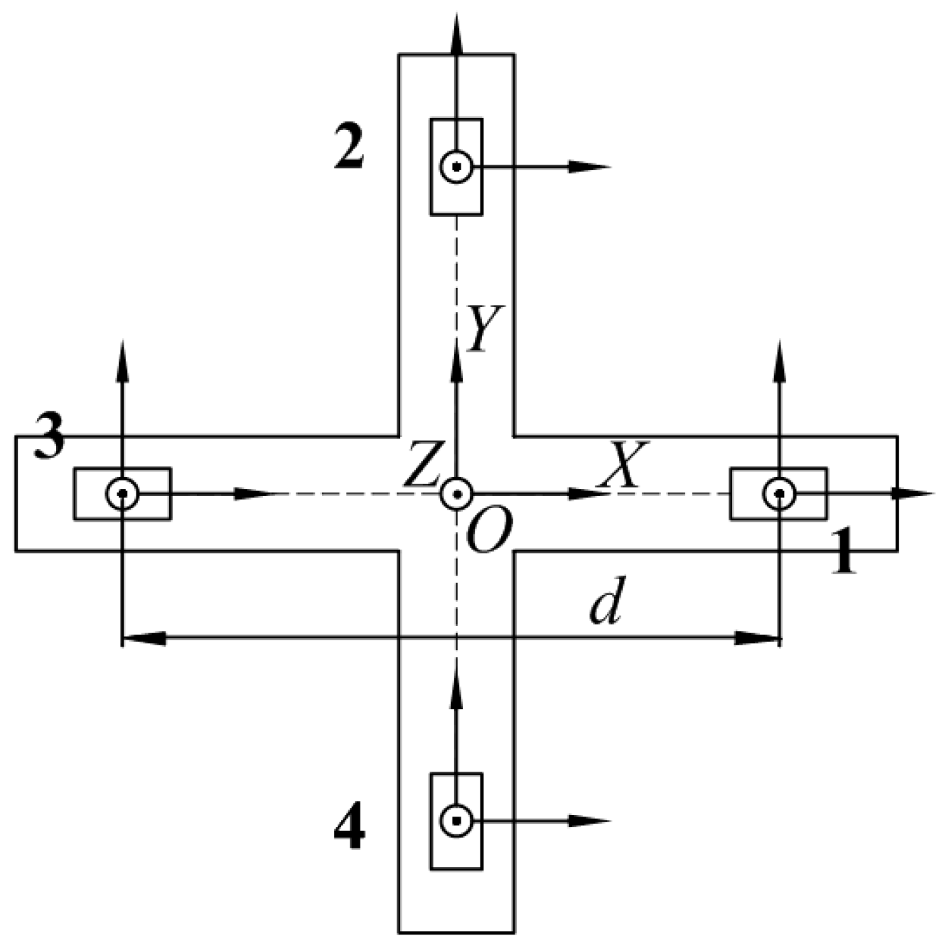
However, it is challenging to measure the gradient of the magnetic vector field in the actual measurement. Therefore, when constructing the magnetic gradient tensor measuring system, the tensor component is estimated using the difference between the measured values of the multiple magnetic sensors. Several different configurations of the magnetic gradient tensor system are analyzed in [
14], and, because of the simple structure, straightforward installation, and minimal structural error, we adopt the planar cross-shaped structure to construct a magnetic gradient tensor system that consists of a planar nonmagnetic platform and four triaxis magnetic sensors. The
x and
y axes lie along the orthogonal baselines, and the
z axis is chosen to make a right-handed Cartesian coordinate system. The baseline distance between two magnetometers in the same direction is
d, as shown in
Figure 1.
We use the short-distance magnetic vector difference method on the baseline to approximate the magnetic tensor gradient as
Bij ≈ Δ
Bi/
dj, where Δ
Bi is the component difference of the two magnetic sensors in the direction
i, and
dj is the distance between the two magnetic sensors in the direction
j; then, the magnetic field vector
Bo at the centre point
O and the magnetic gradient tensor matrix
G can be expressed as
where
Bmn (
m = x,
y,
z;
n = 1, 2, 3, 4) represents the magnetic field component reading of the
nth magnetic sensor in the direction
m. The matrix shown here is not symmetric. Measurement noises and high-order gradients will create differences between the estimates of
Bxy and
Byx. So, we average the two estimates and use a truly symmetric matrix with off-diagonal elements in the actual exploration process, and the tensor
Bxy and
Byx components are treated separately in this paper to achieve more accurate calibration results.
4. Simulation
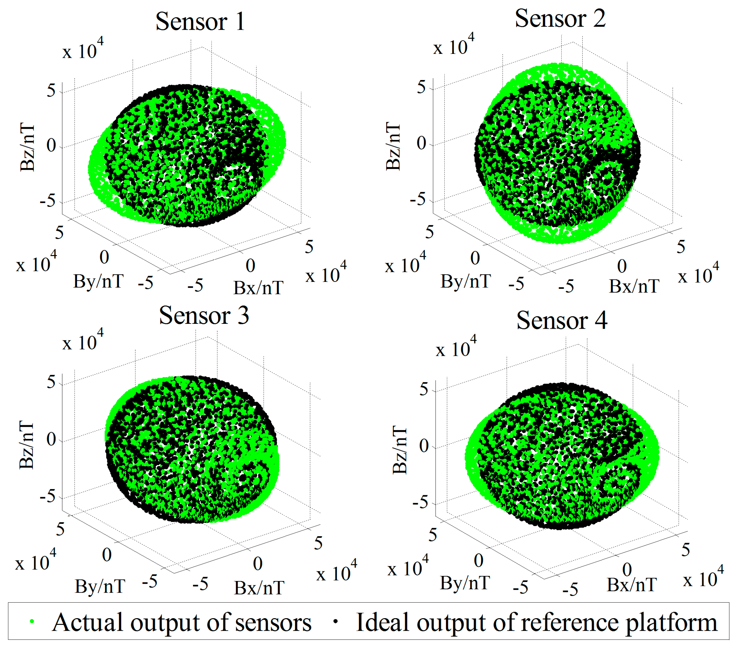
We attempt to verify the performance of the proposed calibration method using MATLAB simulations. We set the total field intensity as 55,000 nT, the magnetic dip as 60°, the magnetic declination as −7°, and the baseline distance of the magnetic gradient tensor system as 0.5 m. To obtain the measured data in the direction of the complete space, the simulated tensor system is rotated around the
X,
Y, and
Z triorthogonal axes in turn at an interval of 20°, sampling the data 18 times per circle. Thus, there is a total of 18
3 posture data sampled in the complete space, which is used as the ideal reference output
B in postures of the full spatial direction of the standard platform. To simulate the rotational noise of the platform in the real measurement, we add Gaussian noise with a mean of 0 nT and a variance of 1 nT in the rotation process of orientations. The 48 error parameters of the four sensors are preset, and the actual tricomponent output of the sensor in the full space orientation is simulated. The tricomponents’ spatial distributions of the sensors’ actual output and the reference platform’s ideal output are contrasted in
Figure 4.
The actual tricomponent of each sensor is calibrated by the proposed method. To compare the calibration performance, we use the simplified linear calibration model of Zhang et al. [
23] and the nonsimplified linear calibration model of Yin et al. [
9]. Before and after the calibration, the TMI output of the sensors and the tensor components of the system center
O-point are shown in
Figure 5 and
Figure 6, respectively, and the root-mean-square errors (RMSE) [
25] of the sensors’ TMI are listed in
Table 1, reflecting the calibration effect of the sensor system error; the RMSE values of the tensor components are listed in
Table 2, reflecting the calibration effect of the misalignment error between axes, and the preset and fitting estimation parameters in simulation are listed in
Table 3.
According to the simulation results, in the case of a uniform magnetic field with no hard or soft magnetic interference, when we use the simplified linear calibration of Zhang et al., the second or higher-order small quantities are neglected in the process of the single magnetometer calibration model, and the calibration deviations are brought in. Relative to the method of Zhang et al., the effect of the calibration of the nonlinear calibration method proposed in this paper is equivalent to that of the nonsimplified two-step linear calibration proposed by Yin et al., with both achieving accurate calibration in the theory of the system error in the Gaussian noise error range. However, this approach does not match the rotation order of solving the misalignment error in the step-by-step process of the linear two-step method, thus causing the estimation accuracy of the parameters to be affected by the deviation of variable conversion; this outcome is an inevitable drawback of the two-step method. The simulation results show that the parameter minimum estimation accuracy (PMEA) of the method of Yin et al. is only 86% [
9], while the PMEA of the proposed nonlinear method is as high as 99.81%, enabling the achievement of the approximate lossless calibration of the error parameter model in the ideal case.
5. Experimental Verification
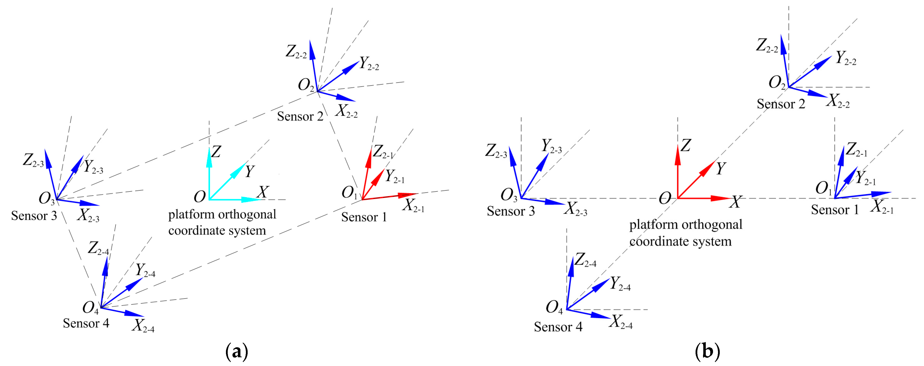
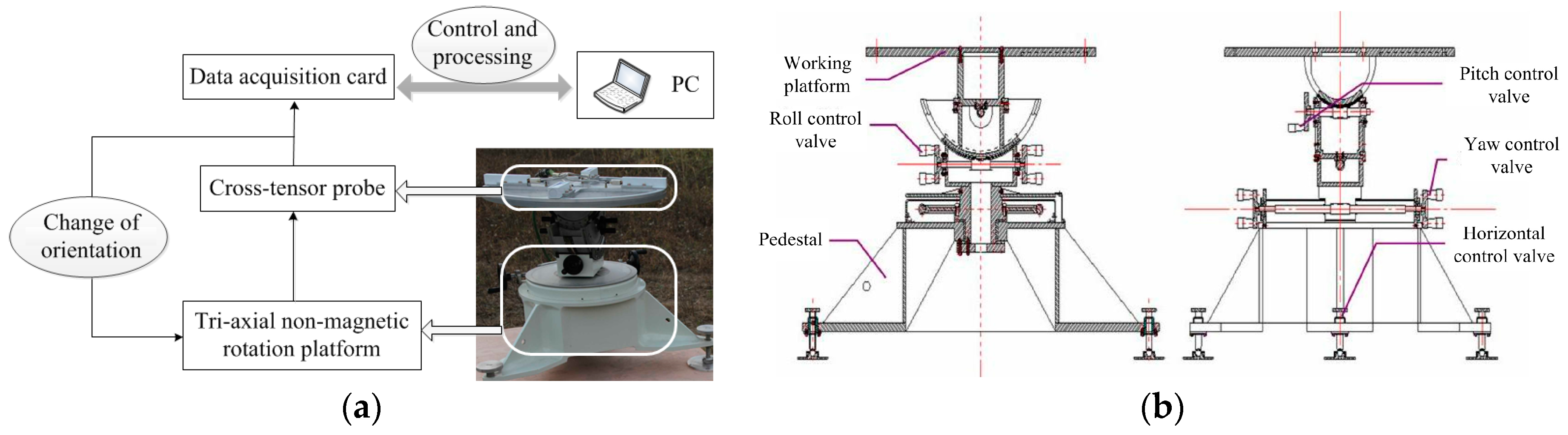
A planar cross-magnetic gradient tensor system is built as shown in
Figure 7a, consisting of four Bartington-produced triaxial fluxgate sensors, an aluminium cross, a triaxial nonmagnetic rotation platform (the structure design is shown in
Figure 7b), a data acquisition card, and a software terminal.
The material of the nonmagnetic rotation platform are aluminum and copper to avoid magnetic interference caused by operating. The main technical parameters of the platform are the following: (1) the orientation rotation range of the roll angle is 360°, and the pitch and yaw angle are ±40°; (2) the position accuracy of three Euler angles is limited to ±6’. Using Altai (Company, Beijing, China) USB2852 signal acquisition card for the data acquisition module, with 16-channel synchronous data acquisition and 16 bits of resolution, the frequency is 31 Hz−250 KHz.
Experiments in a stable environmental field with less magnetic interference were conducted in a suburb of Shijiazhuang, China. The baseline distance of the tensor system was 0.4 m, and the temperature of the working environment was 29 °C. To avoid the influence of geomagnetic diurnal variation as much as possible, the time of the experiment was chosen to be 6:00 pm. Using the scalar proton magnetometer to determine a measurement point with a comparatively more stable uniform magnetic field, the average TMI scale value Bs of the tensor system in the rotating space was 53,902.87 nT, and the range of fluctuation was ±10 nT for different orientations.
The experimental process was divided into two parts, the first being conducted around the
Z-axis of the platform for a standard measurement, and the second being a random orientation measurement, i.e., a random rotation of the nonmagnetic platform for arbitrary space orientation measurement point sampling. Standard measurements were sampled once per 10°, and a total of 36 samples were taken around the
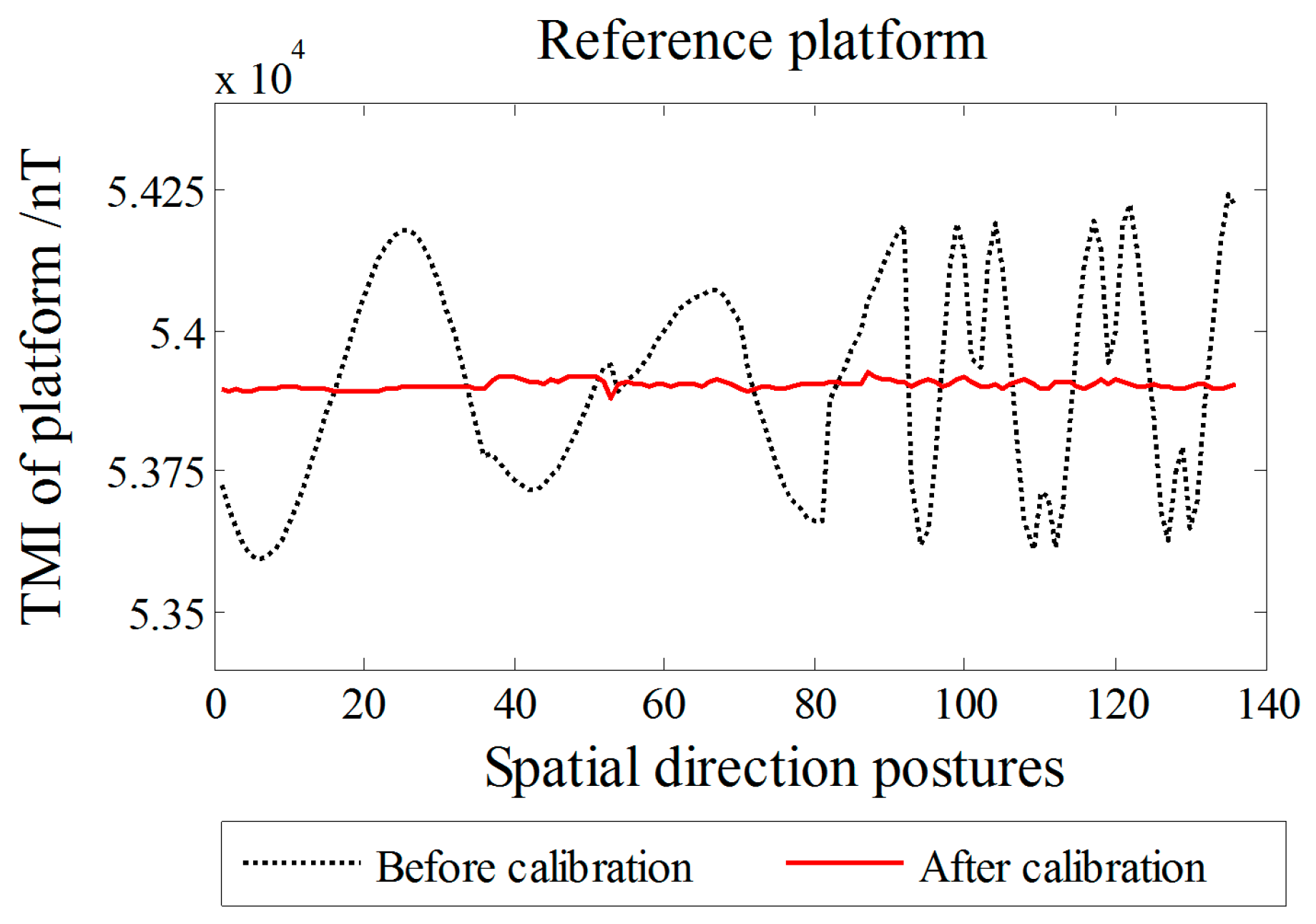
Z-axis per circle. Random sampling was performed a total of 100 times, thus increasing the amount of data to avoid accidental results and ensure the effect and adaptable performance of the calibration. A total of 136 sets of spatial direction posture data were sampled, each of which contains the magnetic field tricomponent output of each orientation for four sensors. According to (2), we obtain an average of tricomponents of the four sensors’ output to
Bo, and we use
Bs as the reference to calibrate
Bo by the linear method of
Section 5, to construct the artificial-reference-platform ideal output
B = (
Bx,
By,
Bz)
T of the cross tensor system center
O-point. A comparison of the reference platform outputs before and after calibration is shown in
Figure 8. The RMSE of the TMI of the artificial platform output
B is 7.4 nT after the calibration, which is within the range of the TMI orientation fluctuation, proving the validity of
B.
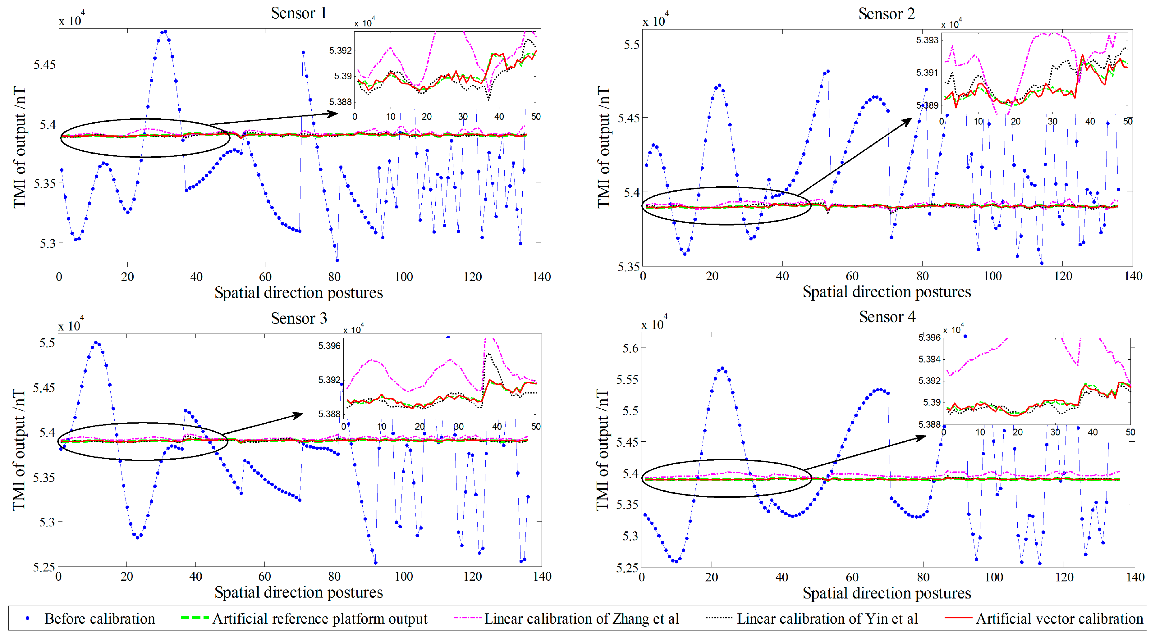
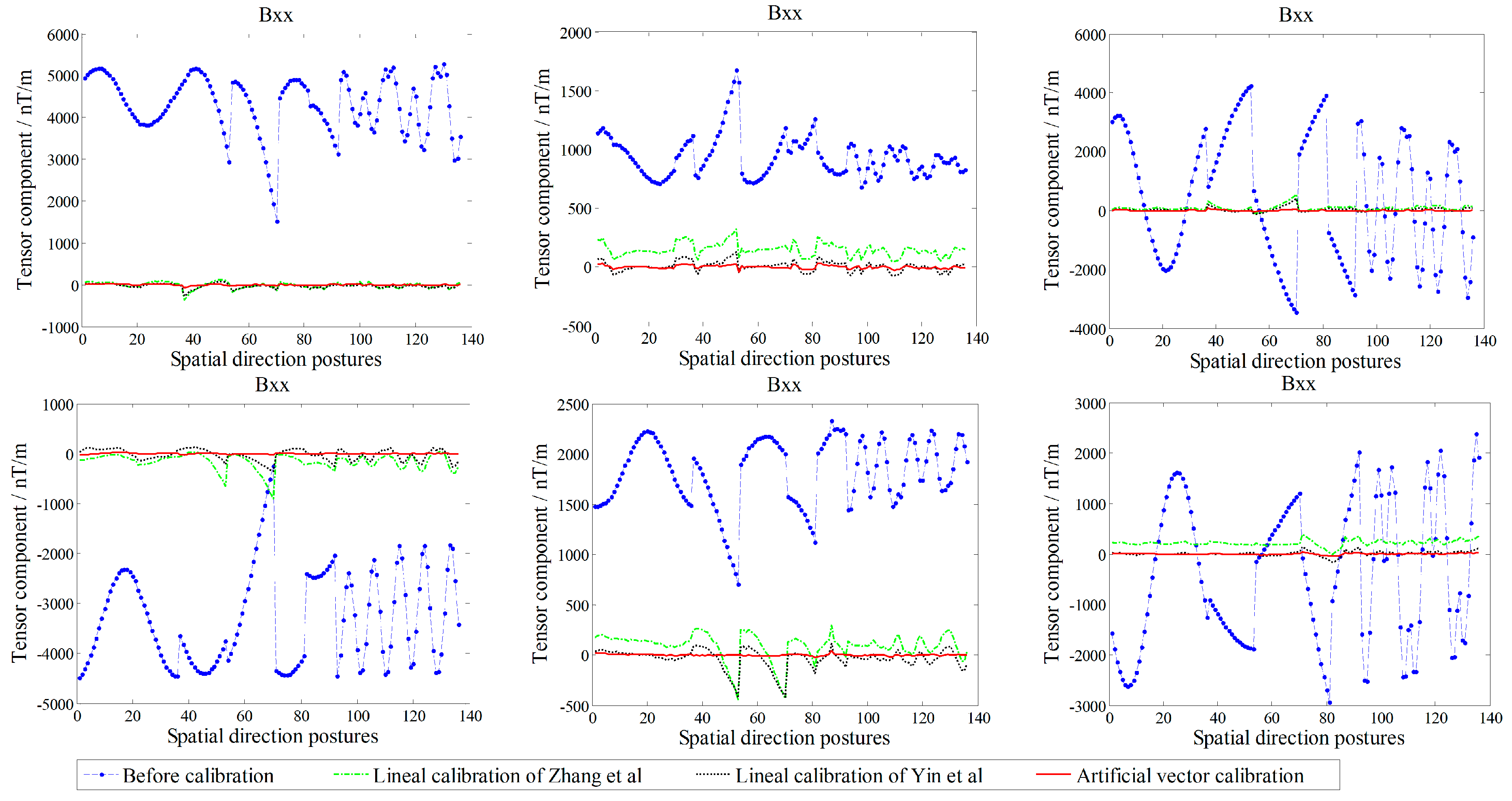
All data were calculated using the linear calibration method of Yin et al., Zhang et al., and the proposed artificial vector calibration method. We calibrated the output of the four sensors after obtaining a total of 48 estimated error parameters. The calibration effect of TMI for each sensor is shown in
Figure 9, with the corresponding RMSE presented in
Table 4. Since the ambient magnetic field is a nonuniform field, and there are diurnal and environmental magnetic interferences, the true field intensity of the geomagnetic field is not constant but fluctuating; therefore, along with the orientation change process, the real geomagnetic total field can be represented by 136 sets of the reference platform output
B and is used as a reference in
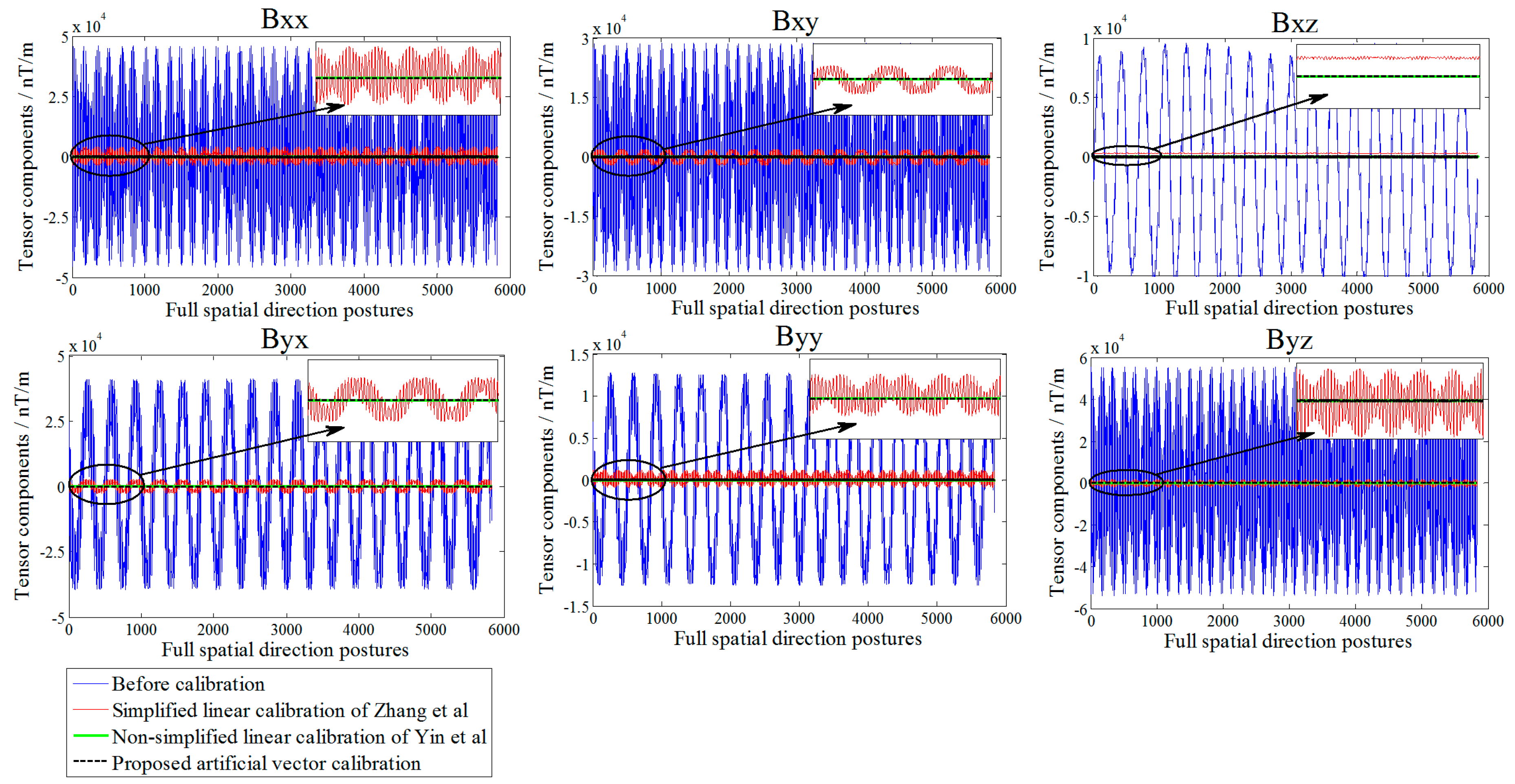
Figure 9. The six independent tensor components of the system before and after calibration are shown in
Figure 10, with the corresponding RMSE values listed in
Table 5. For comparison,
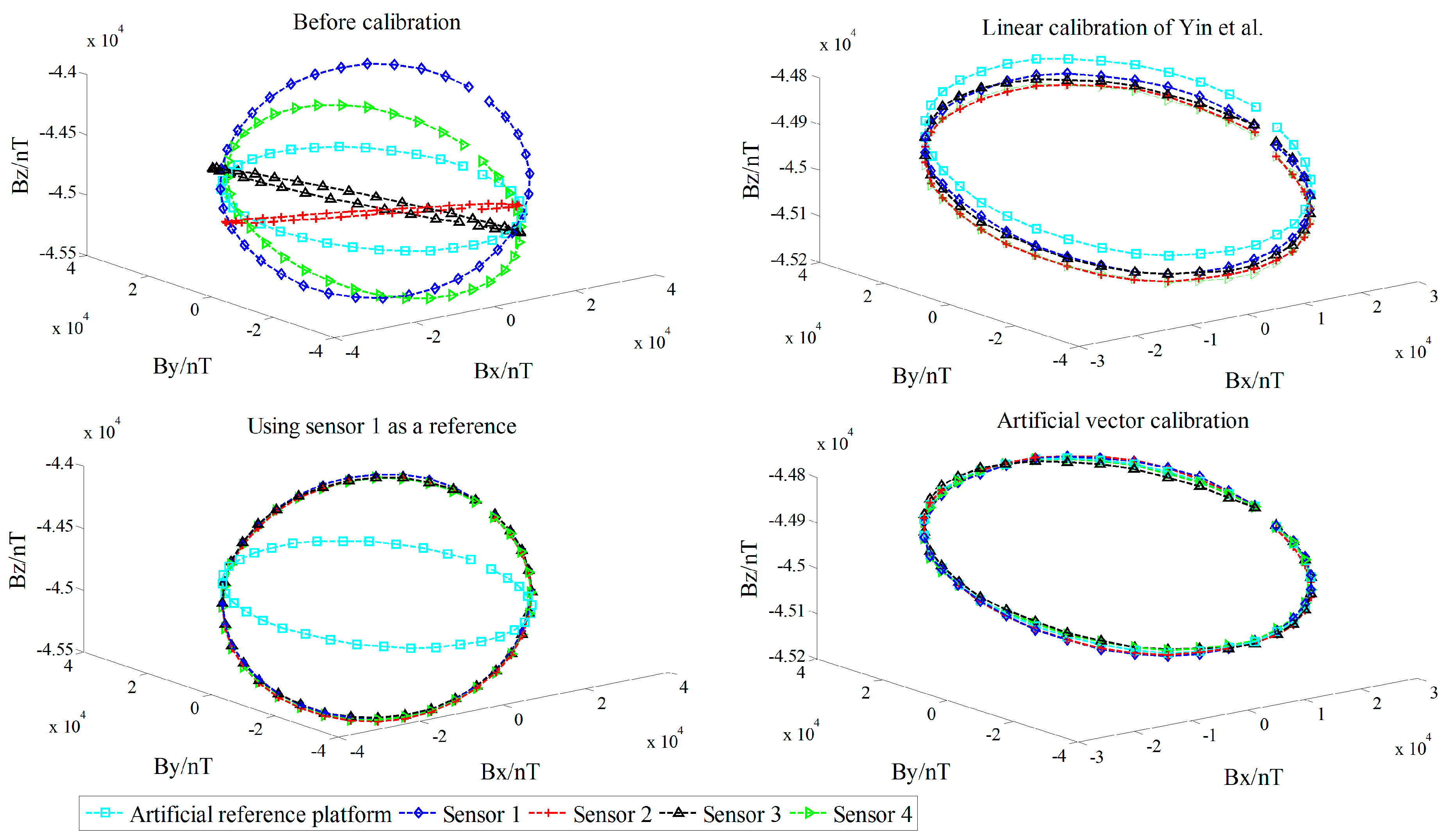
Figure 11 shows the linear calibration of Yin et al. [
9], the aligning idea of Pang et al. [
16] when using one of the sensors as a reference, and the spatial distributions of the sensor’s magnetic field tricomponents before and after calibration of the first 36 orientations of standard measurements rotating around the
Z-axis. The total field output RMSE [
25] is given by:
where
Bi is the reference platform output of the
ith posture point,
is the calibration output of the
ith posture point, and
N is the number of orientations. We can see that the accuracy of the simplified linear calibration of Zhang et al. is slightly worse. The results of the experimental comparison show that we must use
Bs as the reference for the two-step linear calibration of Yin et al. because of the calculation requirements; however, this approach ignores the fluctuation along with the orientation change of the magnetic field intensity in the actual environment, resulting in the OC phenomenon, so that the coaxial output between the sensors and the reference platform is affected after calibration. However, this result is not reflected in the simulation process described in
Section 6 for the OC phenomenon because of the set ideal case. By contrast, the sensor can fit the reference platform output accurately with the proposed vector calibration method, the fluctuant tracking performance is improved, the RMSE of TMI is reduced to less than 1 nT, and the accurate calibration is achieved in the abovementioned average TMI scale fluctuation range of vector calibration. For the misalignment error, the aligning idea of Pang et al. exhibits a satisfactory coaxiality after calibration, but it cannot be output along the reference platform, making this approach impractical, while the performance of the linear method of Yin et al. is affected by the output coincidence degree because of the OC phenomenon for a single sensor. The RMSE of the tensor components is substantially reduced by the proposed method, and the tricomponent spatial distributions of the sensors magnetic field are more coaxial and show a stronger degree of coincidence with the reference platform output.
To verify the robust performance of the 48 error parameters estimated by this method, we reselect the measurement point. The obtained results show that the reproduction degree of each parameter after two estimation iterations is higher than 95% in
Table 6, indicating that the calibration results are stable and reliable.
6. Conclusions
This paper proposes an artificial vector calibration method for differencing magnetic gradient tensor systems. We use the linear calibration method to construct the artificial ideal platform output as the reference vector. The Levenberg–Marquardt algorithm is used to realize the least-squares fitting of nonlinear equations by establishing an integrated nonlinear mathematical model of the single-sensor system error of biases, scale factors, nonorthogonal angles, and the measurement error of the sensor arrays. A total of 48 parameters of the four sensors is estimated simultaneously, providing the concept and method for the accurate calibration of aeronautical, underwater, and surface tensor magnetic measuring instruments. As a result of using the multiorientation single-sensor vector output calibration, the method is suitable for any triaxial magnetic sensor or accelerometer array combination of the magnetic field, and the gravity field tensor system with an accurate and efficient parameter estimation can achieve batch and rapid calibration of tensor measurement instruments, contributing to the scientific literature and the commercial value. Relative to the calibration methods of Zhang et al., Yin et al., and Pang et al., in the ideal case of a uniform magnetic field, the accuracy of parameter estimation with the nonlinear integrated calibration is close to 100% in simulation, and a lossless calibration is realized. As a result of the lack of the integrated parameter model, the defects of the fixed solving sequence and distortion of conversion in the two-step method are inevitable, while, experimentally, the ability of tracking the calibration for the magnetic field output fluctuates, following the orientation change with the proposed method, effectively avoiding the OC problem of the linear calibration, which must set the total field intensity to a constant value to solve the linear equations.
In this paper, the idea and method of a low-cost vector calibration for tensor systems are provided, and the estimation of the parameters is comparatively accurate. However, we have not considered the influence of the sensor temperature coefficient, nonlinearity, or hard or soft magnetic interference on the accuracy of the tensor system, and the algorithm has a strong dependence on vector output based on the standard reference platform. In the future, multiorientation magnetic field vector measurement data can be used as the tensor system reference outputs with a more sensitive and high-frame magnetometer to improve the calibration accuracy and reliability.


