Classification of Rice Heavy Metal Stress Levels Based on Phenological Characteristics Using Remote Sensing Time-Series Images and Data Mining Algorithms

Abstract
:1. Introduction
2. Materials
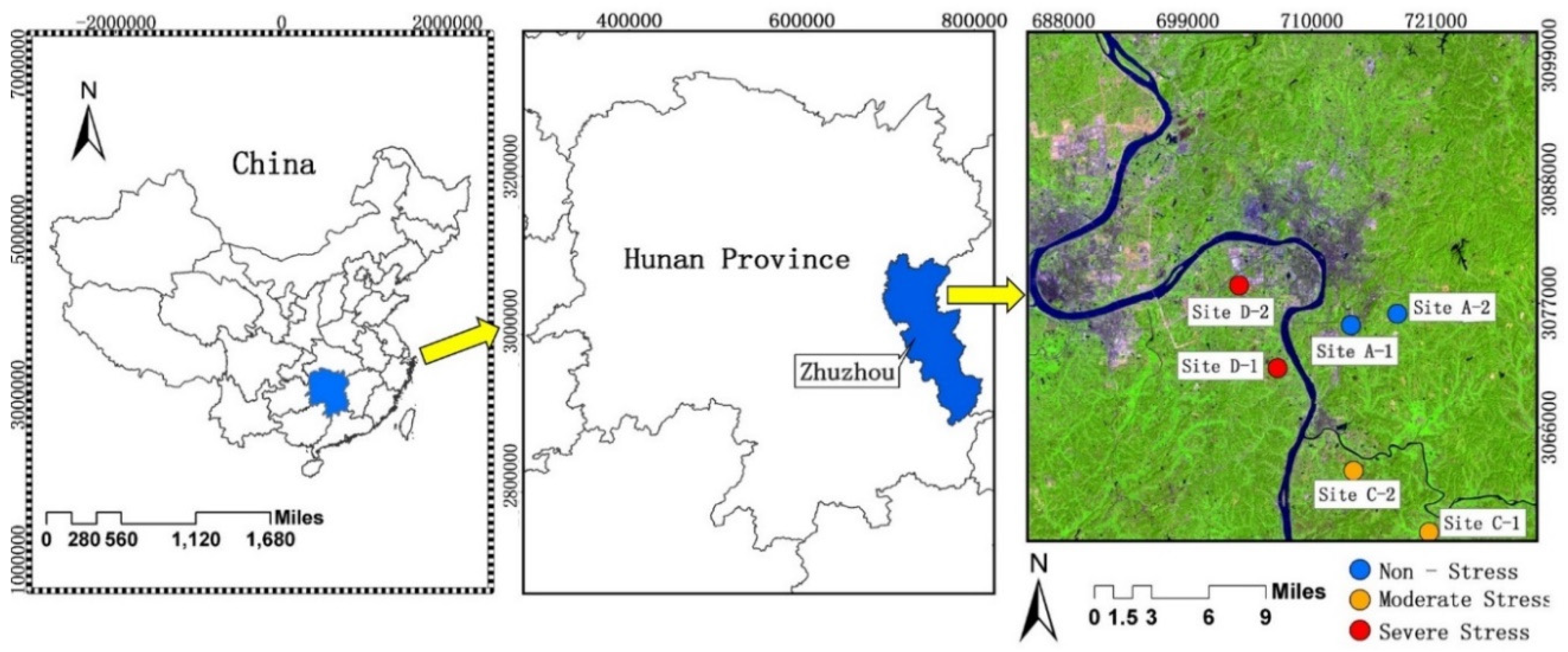
2.1. Study Area
2.2. Data Preparation
3. Methods
3.1. Construction of VI Time Series for Phenological Analysis
3.2. Designing Phenological Metrics from Seasonal Patterns of VIs
3.3. Classification of Heavy Metal Stress Levels in Rice
3.4. Accuracy Assessment
4. Results
4.1. Rice Growth Trajectory under Different Heavy Metal Stress
4.2. Identification of Optimal Number of Feature Subset
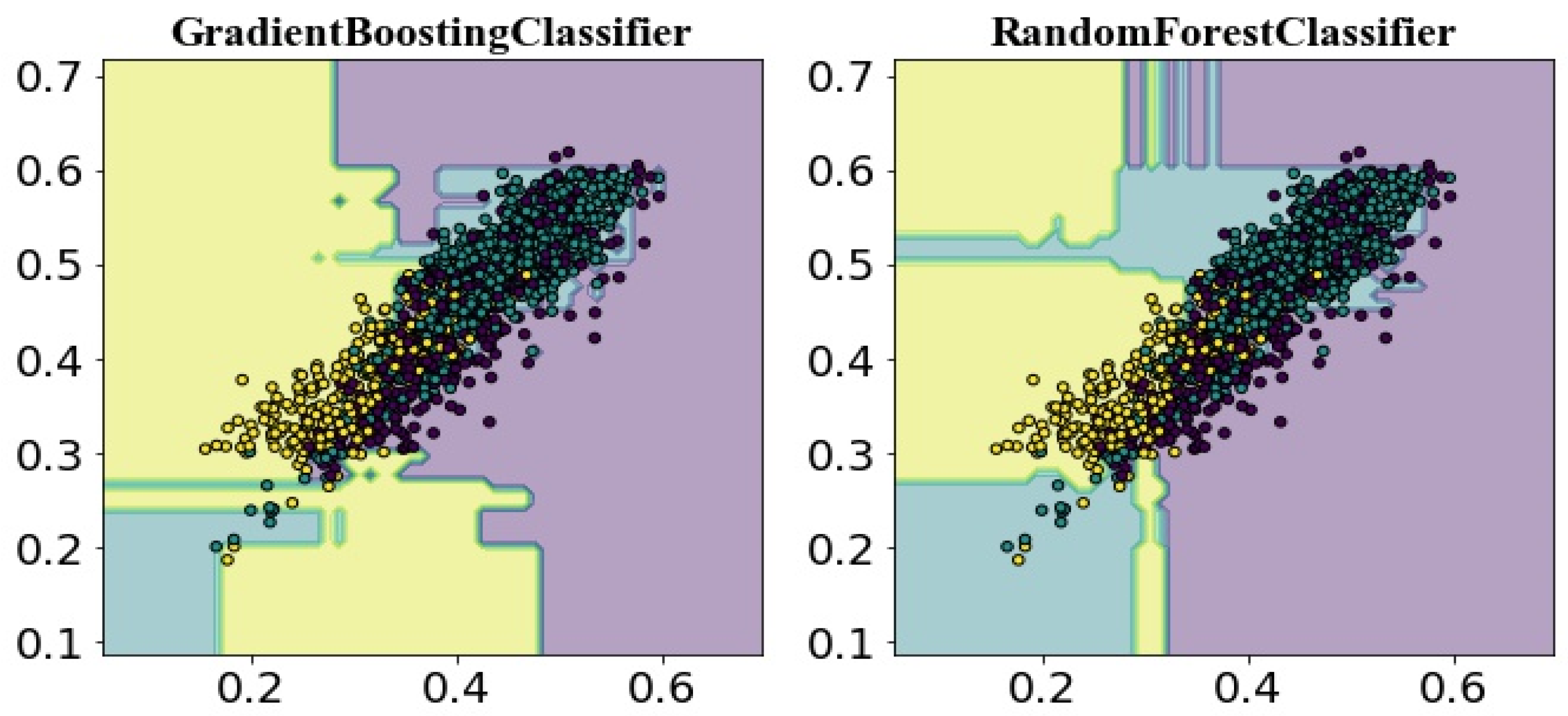
4.3. Classification Results of Stress Levels
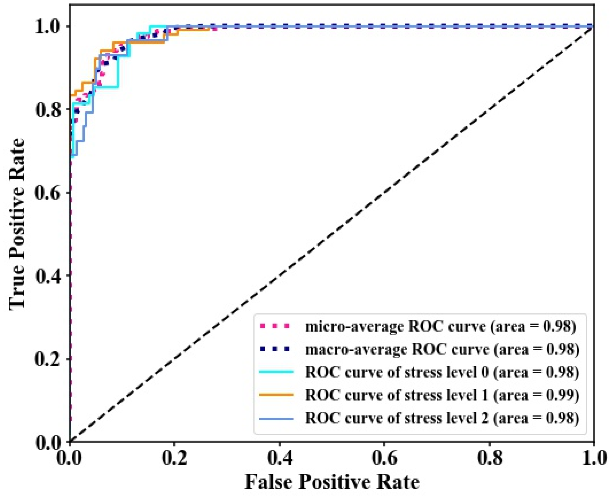
4.4. Validation of Discrimination Results
5. Discussion
6. Conclusions
Author Contributions
Funding
Conflicts of Interest
References
- Zhang, X.; Zhong, T.; Liu, L.; Ouyang, X. Impact of Soil Heavy Metal Pollution on Food Safety in China. PLoS ONE 2015, 10, e0135182. [Google Scholar] [CrossRef] [PubMed]
- Jianming, X.U.; Meng, J.; Liu, X.; Shi, J.; Tang, X. Control of Heavy Metal Pollution in Farmland of China in Terms of Food Security. Bull. Chin. Acad. Sci. 2018, 33, 153–159. [Google Scholar]
- Zhao, J.X.; Yin, P.C.; Yue, R. Research Progress of Status, Source, Restoration Technique of Heavy Metals Pollution in Cropland of China. J. Anhui Agric. Sci. 2018, 46, 19–21. [Google Scholar]
- Järup, L. Hazards of heavy metal contamination. Br. Med. Bull. 2003, 68, 167–182. [Google Scholar] [CrossRef] [PubMed] [Green Version]
- Liu, X.; Zhong, L.; Meng, J.; Fan, W.; Zhang, J.; Zhi, Y.; Zeng, L.; Tang, X.; Xu, J. A multi-medium chain modeling approach to estimate the cumulative effects of cadmium pollution on human health. Environ. Pollut. 2018, 239, 308–317. [Google Scholar] [CrossRef] [PubMed]
- Chen, W.; Yang, Y.; Xie, T.; Wang, M.; Peng, C.; Wang, R. Challenges and Countermeasures for Heavy Metal Pollution Control in Farmlands of China. Acta Pedol. Sin. 2018, 55, 261–272. [Google Scholar]
- Wanlu, L.; Binbin, X.; Qiujin, S.; Xingmei, L.; Jianming, X.; Brookes, P.C. The identification of ‘hotspots’ of heavy metal pollution in soil-rice systems at a regional scale in eastern China. Sci. Total Environ. 2014, 472, 407–420. [Google Scholar]
- Deng-Wei, W.; Yun-Zhao, W.; Hong-Rui, M. Review on Remote Sensing Monitoring on Contaminated Plant. Remote Sens. Technol. Appl. 2009, 24, 238–245. [Google Scholar]
- Jin, M.; Liu, X.; Zhang, B. Evaluating Heavy-Metal Stress Levels in Rice Using a Theoretical Model of Canopy-Air Temperature and Leaf Area Index Based on Remote Sensing. IEEE J. Sel. Top. Appl. Earth Obs. Remote Sens. 2017, 10, 1–11. [Google Scholar] [CrossRef]
- Liu, M.; Wang, T.; Skidmore, A.K.; Liu, X. Heavy metal-induced stress in rice crops detected using multi-temporal Sentinel-2 satellite images. Sci. Total Environ. 2018, 637–638, 18–29. [Google Scholar] [CrossRef]
- Ren, H.Y.; Zhuang, D.F.; Pan, J.J.; Shi, X.Z.; Wang, H.J. Hyper-spectral remote sensing to monitor vegetation stress. J. Soils Sediments 2008, 8, 323–326. [Google Scholar] [CrossRef] [Green Version]
- Barcelo, J.; Poschenrieder, C. Plant water relations as affected by heavy metal stress: A review. J. Plant Nutr. 1990, 13, 1–37. [Google Scholar] [CrossRef]
- Cheng, S. Effects of Heavy metals on plants and resistance mechanisms. Environ. Sci. Pollut. Res. 2003, 10, 256–264. [Google Scholar] [CrossRef] [Green Version]
- Dias, M.C.; Monteiro, C.; Moutinho-Pereira, J.; Correia, C.; Gonçalves, B.; Santos, C. Cadmium toxicity affects photosynthesis and plant growth at different levels. Acta Physiol. Plant. 2013, 35, 1281–1289. [Google Scholar] [CrossRef]
- Nagajyoti, P.C.; Lee, K.D.; Sreekanth, T.V.M. Heavy metals, occurrence and toxicity for plants: A review. Environ. Chem. Lett. 2010, 8, 199–216. [Google Scholar] [CrossRef]
- Liu, S.; Liu, X.; Liu, M.; Wu, L.; Ding, C.; Huang, Z. Extraction of Rice Phenological Differences under Heavy Metal Stress Using EVI Time-Series from HJ-1A/B Data. Sensors 2017, 17, 1243. [Google Scholar] [Green Version]
- Liu, T.; Liu, X.; Liu, M.; Wu, L. Evaluating Heavy Metal Stress Levels in Rice Based on Remote Sensing Phenology. Sensors 2018, 18, 860. [Google Scholar] [CrossRef] [PubMed]
- Tian, L.; Liu, X.; Zhang, B.; Liu, M.; Wu, L. Extraction of Rice Heavy Metal Stress Signal Features Based on Long Time Series Leaf Area Index Data Using Ensemble Empirical Mode Decomposition. Int. J. Environ. Res. Public Health 2017, 14, 1018. [Google Scholar] [CrossRef]
- Cao, R.; Chen, J.; Shen, M.; Tang, Y. An improved logistic method for detecting spring vegetation phenology in grasslands from MODIS EVI time-series data. Agric. Forest Meteorol. 2015, 200, 9–20. [Google Scholar] [CrossRef]
- Melaas, E.K.; Friedl, M.A.; Zhu, Z. Detecting interannual variation in deciduous broadleaf forest phenology using Landsat TM/ETM + data. Remote Sens. Environ. 2013, 132, 176–185. [Google Scholar] [CrossRef]
- Sakamoto, T.; Yokozawa, M.; Toritani, H.; Shibayama, M.; Ishitsuka, N.; Ohno, H. A crop phenology detection method using time-series MODIS data. Remote Sens. Environ. 2005, 96, 366–374. [Google Scholar] [CrossRef]
- Walker, J.J.; Beurs, K.M.D.; Wynne, R.H.; Gao, F. Evaluation of Landsat and MODIS data fusion products for analysis of dryland forest phenology. Remote Sens. Environ. 2012, 117, 381–393. [Google Scholar] [CrossRef]
- Gao, F.; Masek, J.; Schwaller, M.; Hall, F. On the blending of the Landsat and MODIS surface reflectance: Predicting daily Landsat surface reflectance. IEEE Trans. Geosci. Remote Sens. 2006, 44, 2207–2218. [Google Scholar]
- Hilker, T.; Wulder, M.A.; Coops, N.C.; Linke, J.; Mcdermid, G.; Masek, J.G.; Gao, F.; White, J.C. A new data fusion model for high spatial- and temporal-resolution mapping of forest disturbance based on Landsat and MODIS. Remote Sens. Environ. 2009, 113, 1613–1627. [Google Scholar] [CrossRef]
- Weng, Q.; Fu, P.; Gao, F. Generating daily land surface temperature at Landsat resolution by fusing Landsat and MODIS data. Remote Sens. Environ. 2014, 145, 55–67. [Google Scholar] [CrossRef]
- Zhu, X.L.; Jin, C.; Feng, G.; Chen, X.H.; Masek, J.G. An enhanced spatial and temporal adaptive reflectance fusion model for complex heterogeneous regions. Remote Sens. Environ. 2010, 114, 2610–2623. [Google Scholar] [CrossRef]
- Reed, B.C.; Brown, J.F.; Vanderzee, D.; Loveland, T.R.; Merchant, J.W.; Ohlen, D.O. Measuring phenological variability from satellite imagery. J. Veg. Sci. 1994, 5, 703–714. [Google Scholar] [CrossRef]
- Reed, B.C.; White, M.; Brown, J.F. Remote Sensing Phenology; Springer: Dordrecht, The Netherlands, 2003; pp. 365–381. [Google Scholar]
- Cong, N.; Piao, S.; Chen, A.; Wang, X.; Lin, X.; Chen, S.; Han, S.; Zhou, G.; Zhang, X. Spring vegetation green-up date in China inferred from SPOT NDVI data: A multiple model analysis. Agric. Forest Meteorol. 2012, 165, 104–113. [Google Scholar] [CrossRef]
- Mo, Y.; Momen, B.; Kearney, M.S. Quantifying moderate resolution remote sensing phenology of Louisiana coastal marshes. Ecol. Model. 2015, 312, 191–199. [Google Scholar] [CrossRef]
- Pan, Z.; Huang, J.; Zhou, Q.; Wang, L.; Cheng, Y.; Zhang, H.; Blackburn, G.A.; Yan, J.; Liu, J. Mapping crop phenology using NDVI time-series derived from HJ-1 A/B data. Int. J. Appl. Earth Obs. Geoinf. 2015, 34, 188–197. [Google Scholar] [CrossRef] [Green Version]
- Atkinson, P.M.; Jeganathan, C.; Dash, J.; Atzberger, C. Inter-comparison of four models for smoothing satellite sensor time-series data to estimate vegetation phenology. Remote Sens. Environ. 2012, 123, 400–417. [Google Scholar] [CrossRef]
- Hird, J.N.; Mcdermid, G.J. Noise reduction of NDVI time series: An empirical comparison of selected techniques. Remote Sens. Environ. 2009, 113, 248–258. [Google Scholar] [CrossRef]
- Vilela, M.; Borges, C.C.; Vinga, S.; Vasconcelos, A.T.R.; Santos, H.; Voit, E.O.; Almeida, J.S. Automated smoother for the numerical decoupling of dynamics models. BMC Bioinform. 2007, 8, 305. [Google Scholar] [CrossRef] [PubMed]
- Ling, Y.; Geng, L.N.; Jing, Y.S.; Rong-Chen, H.U.; Sun, X.; Bureau, J.M. Study on Phenology Extraction of Paddy Rice Based on Different Filtering Methods. Sci. Technol. Eng. 2014, 14, 1671–1815. [Google Scholar]
- Sun, H.S.; Huang, J.F.; Peng, D.L. Detecting major growth stages of paddy rice using MODIS data. J. Remote Sens. 2009, 6, 1122–1137. [Google Scholar]
- Dong, J.; Xiao, X.; Menarguez, M.A.; Zhang, G.; Qin, Y.; Thau, D.; Biradar, C.; Iii, B.M. Mapping paddy rice planting area in northeastern Asia with Landsat 8 images, phenology-based algorithm and Google Earth Engine. Remote Sens. Environ. 2016, 185, 142–154. [Google Scholar] [CrossRef] [Green Version]
- Zhang, G.; Xiao, X.; Dong, J.; Kou, W.; Jin, C.; Qin, Y.; Zhou, Y.; Wang, J.; Menarguez, M.A.; Biradar, C. Mapping paddy rice planting areas through time series analysis of MODIS land surface temperature and vegetation index data. Isprs J. Photogramm. Remote Sens. 2015, 106, 157–171. [Google Scholar] [CrossRef] [Green Version]
- Zhou, Y.; Xiao, X.; Qin, Y.; Dong, J.; Zhang, G.; Kou, W.; Jin, C.; Wang, J.; Li, X. Mapping paddy rice planting area in rice-wetland coexistent areas through analysis of Landsat 8 OLI and MODIS images. Int. J. Appl. Earth Obs. Geoinf. 2016, 46, 1–12. [Google Scholar] [CrossRef] [Green Version]
- Küçük, Ç.; Taşkın, G.; Erten, E. Paddy-Rice Phenology Classification Based on Machine-Learning Methods Using Multitemporal Co-Polar X-Band SAR Images. IEEE J. Sel. Top. Appl. Earth Obs. Remote Sens. 2017, 9, 2509–2519. [Google Scholar] [CrossRef]
- Chen, J.; Chen, J.; Liao, A.; Cao, X.; Chen, L.; Chen, X.; He, C.; Han, G.; Peng, S.; Lu, M. Global land cover mapping at 30 m resolution: A POK-based operational approach. ISPRS J. Photogramm. Remote Sens. 2015, 103, 7–27. [Google Scholar] [CrossRef]
- Du, P.; Samat, A.; Waske, B.; Liu, S.; Li, Z. Random Forest and Rotation Forest for fully polarized SAR image classification using polarimetric and spatial features. ISPRS J. Photogramm. Remote Sens. 2015, 105, 38–53. [Google Scholar] [CrossRef]
- Luo, J.; Li, X.; Ma, R.; Li, F.; Duan, H.; Hu, W.; Qin, B.; Huang, W. Applying remote sensing techniques to monitoring seasonal and interannual changes of aquatic vegetation in Taihu Lake, China. Ecol. Indic. 2016, 60, 503–513. [Google Scholar] [CrossRef]
- Miao, X.; Heaton, J.S.; Zheng, S.; Charlet, D.A.; Liu, H. Applying tree-based ensemble algorithms to the classification of ecological zones using multi-temporal multi-source remote-sensing data. Int. J. Remote Sens. 2012, 33, 1823–1849. [Google Scholar] [CrossRef]
- Schneider, A. Monitoring land cover change in urban and peri-urban areas using dense time stacks of Landsat satellite data and a data mining approach. Remote Sens. Environ. 2012, 124, 689–704. [Google Scholar] [CrossRef]
- Chen, D.; Guo, H.; Li, R.; Li, L.; Pan, G.; Chang, A.; Joseph, S. Low uptake affinity cultivars with biochar to tackle Cd-tainted rice—A field study over four rice seasons in Hunan, China. Sci. Total Environ. 2016, 541, 1489–1498. [Google Scholar] [CrossRef] [PubMed]
- Lei, M.; Tie, B.Q.; Song, Z.G.; Liao, B.H.; Lepo, J.E.; Huang, Y.Z. Heavy metal pollution and potential health risk assessment of white rice around mine areas in Hunan Province, China. Food Secur. 2015, 7, 45–54. [Google Scholar] [CrossRef]
- Linghong, K.E.; Wang, Z.; Song, C.; Zhenquan, L.U. Reconstruction of MODIS LST Time Series and Comparison with Land Surface Temperature (T) among Observation Stations in the Northeast Qinghai-Tibet Plateau. Prog. Geogr. 2011, 30, 819–826. [Google Scholar]
- Wang, Q.; Huang, C.; Liu, G.; Liu, Q.; He, L.I.; Chen, Z. Cloud Shadow Identification Based on QA Band of Landsat 8. J. Geo-Inf. Sci. 2018, 20, 89–98. [Google Scholar]
- Gao, B.C. NDWI—A normalized difference water index for remote sensing of vegetation liquid water from space. Remote Sens. Environ. 1996, 58, 257–266. [Google Scholar] [CrossRef]
- Huete, A.; Didan, K.; Miura, T.; Rodriguez, E.P.; Gao, X.; Ferreira, L.G. Overview of the radiometric and biophysical performance of the MODIS vegetation indices. Remote Sens. Environ. 2002, 83, 195–213. [Google Scholar] [CrossRef]
- Xiao, X.; Boles, S.; Liu, J.; Zhuang, D.; Frolking, S.; Li, C.; Salas, W.; Iii, B.M. Mapping paddy rice agriculture in southern China using multi-temporal MODIS images. Remote Sens. Environ. 2005, 95, 480–492. [Google Scholar] [CrossRef]
- Eilers, P.H.C. A Perfect Smoother. Anal. Chem. 2003, 75, 3631–3636. [Google Scholar] [CrossRef] [PubMed]
- Atzberger, C.; Rembold, F. Estimation of inter-annual winter crop area variation and spatial distribution with low resolution NDVI data by using neural networks trained on high resolution images. In Proceedings of the Remote Sensing for Agriculture, Ecosystems, and Hydrology XI, Berlin, Germany, 1–3 September 2009; pp. 170–175. [Google Scholar]
- Atzberger, C.; Eilers, P.H.C. Evaluating the Effectiveness of Smoothing Algorithms in the Absence of Ground Reference Measurements; Taylor & Francis, Inc.: Abingdon, UK, 2011; pp. 3689–3709. [Google Scholar]
- Atzberger, C.; Eilers, P.H.C. A time series for monitoring vegetation activity and phenology at 10-daily time steps covering large parts of South America. Int. J. Digit. Earth 2011, 4, 365–386. [Google Scholar] [CrossRef]
- Jönsson, P.; Eklundh, L. TIMESAT—A program for analyzing time-series of satellite sensor data. Comput. Geosci. 2004, 30, 833–845. [Google Scholar] [CrossRef]
- Eklundha, L.; Jönssonb, P. TIMESAT 3.1 Software Manual. Available online: http://web.nateko.lu.se/timesat/docs/timesat3_1_1_SoftwareManual.pdf (accessed on 13 December 2018).
- Christ, M.; Braun, N.; Neuffer, J.; Kempa-Liehr, A.W. Time Series FeatuRe Extraction on basis of Scalable Hypothesis tests (tsfresh—A Python package). Neurocomputing 2018, 307, 72–77. [Google Scholar] [CrossRef]
- Christ, M.; Kempaliehr, A.W.; Feindt, M. Distributed and parallel time series feature extraction for industrial big data applications. arXiv, 2016; arXiv:1610.07717. [Google Scholar]
- Cai, J.; Luo, J.; Wang, S.; Yang, S. Feature selection in machine learning: A new perspective. Neurocomputing 2018, 300, 70–79. [Google Scholar] [CrossRef]
- Varnek, A. 14. Compound Classification Using the Scikit-Learn Library; John Wiley & Sons, Ltd.: Hoboken, NJ, USA, 2017; pp. 223–239. [Google Scholar]
- Hikaru, M.; Seiichiro, A.; Tomomasa, N.; Yoshifumi, O. Accurate and robust gene selection for disease classification using a simple statistic. Bioinformation 2008, 3, 68–71. [Google Scholar]
- Wang, X.; Nagashima, T.; Fukuta, K.; Okada, Y.; Sawai, M.; Tanaka, H.; Uozumi, T. Statistical method for classifying cries of baby based on pattern recognition of power spectrum. Int. J. Biom. 2010, 2, 113–123. [Google Scholar] [CrossRef]
- Defries, R.S.; Chan, J.C.W. Multiple criteria for evaluating machine learning algorithms for land cover classification from satellite data. Remote Sens. Environ. 2000, 74, 503–515. [Google Scholar] [CrossRef]
- Ping, Y.P.; Zang, S.Y. Crop Identification Based on MODIS NDVI Time-series Data and Phenological Characteristics. J. Nat. Resour. 2016, 31, 503–513. [Google Scholar]
- Lewis, H.G.; Brown, M. A generalized confusion matrix for assessing area estimates from remotely sensed data. Int. J. Remote Sens. 2001, 22, 3223–3235. [Google Scholar] [CrossRef] [Green Version]
- Davis, J.; Goadrich, M. The relationship between Precision-Recall and ROC curves. In Proceedings of the International Conference on Machine Learning (ICML ′06), New York, NY, USA, 25–29 June 2006; pp. 233–240. [Google Scholar]


| Study Sites | Geographic Location | Cd Concentration in Soil | Background Value | National Quality Standard | Pollution Level |
|---|---|---|---|---|---|
| A-1 | 113°12′ E 27°47′ N | 0.84 | 1.43 | 0.3–1.0 | None |
| A-2 | 113°10′ E 27°47′ N | 0.84 | None | ||
| C-1 | 113°14′ E 27°37′ N | 2.25 | Moderate | ||
| C-2 | 113°10′ E 27°40′ N | 2.31 | Moderate | ||
| D-1 | 113°06′ E 27°45′ N | 3.27 | Severe | ||
| D-2 | 113°04′ E 27°49′ N | 3.54 | Severe |
| Feature Category | Parameters | Number of Parameters |
|---|---|---|
| Phenological signatures | Annual average, maximum and minimum values of VIs | 18 |
| Base level, seasonal amplitude, seasonal integral, seasonal length and growth ratio | 10 | |
| VIs(heading)-VIs(maturity) | 6 | |
| VIs(heading)-VIs(tillering) | 6 | |
| T(heading)-T(transplantend); | 2 | |
| (NDWImax-NDWImin)/(VI(heading)-VI(maturity)) | 2 | |
| (NDWImax-NDWImin)/(VI(heading)-VI(tillering)) | 2 | |
| Total | 46 |
| Assessment Measures | Random Forest | Gradient Boosting |
|---|---|---|
| Overall Accuracy | 67.57% | 66.12% |
| Correct-Judgement Rate for Non-Stress Rice | 51.94% | 48.70% |
| Correct-Judgement Rate for Moderate-Stress Rice | 79.52% | 78.16% |
| Correct-Judgement Rate for Severe-Stress Rice | 57.14% | 58.10% |
© 2018 by the authors. Licensee MDPI, Basel, Switzerland. This article is an open access article distributed under the terms and conditions of the Creative Commons Attribution (CC BY) license (http://creativecommons.org/licenses/by/4.0/).
Share and Cite
Liu, T.; Liu, X.; Liu, M.; Wu, L. Classification of Rice Heavy Metal Stress Levels Based on Phenological Characteristics Using Remote Sensing Time-Series Images and Data Mining Algorithms. Sensors 2018, 18, 4425. https://doi.org/10.3390/s18124425
Liu T, Liu X, Liu M, Wu L. Classification of Rice Heavy Metal Stress Levels Based on Phenological Characteristics Using Remote Sensing Time-Series Images and Data Mining Algorithms. Sensors. 2018; 18(12):4425. https://doi.org/10.3390/s18124425
Chicago/Turabian StyleLiu, Tianjiao, Xiangnan Liu, Meiling Liu, and Ling Wu. 2018. "Classification of Rice Heavy Metal Stress Levels Based on Phenological Characteristics Using Remote Sensing Time-Series Images and Data Mining Algorithms" Sensors 18, no. 12: 4425. https://doi.org/10.3390/s18124425