Time-Matching Random Finite Set-Based Filter for Radar Multi-Target Tracking

Abstract
1. Introduction
2. Background
2.1. Random Finite Set and Bayesian Multi-Target Filter
2.2. Sampling Time Diversity in Radar Applications
3. Time-Matching RFS-Based MTT
3.1. Time-Matching Bayesian Filtering
3.2. Time-Matching Joint-GLMB Filter
3.3. Time-Matching PHD Filter
4. Simulations
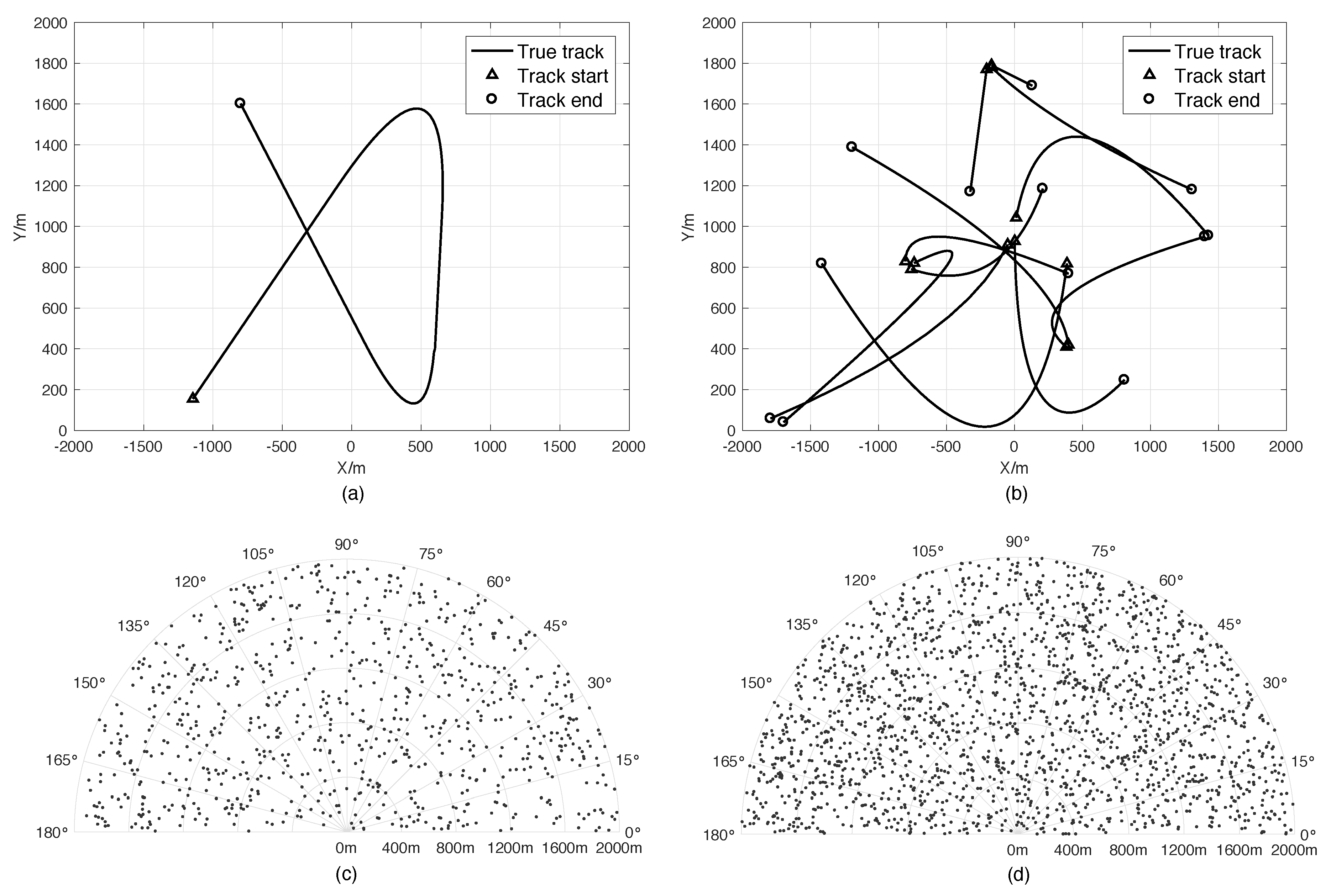
4.1. Scenarios
4.2. Target Tracking Setup
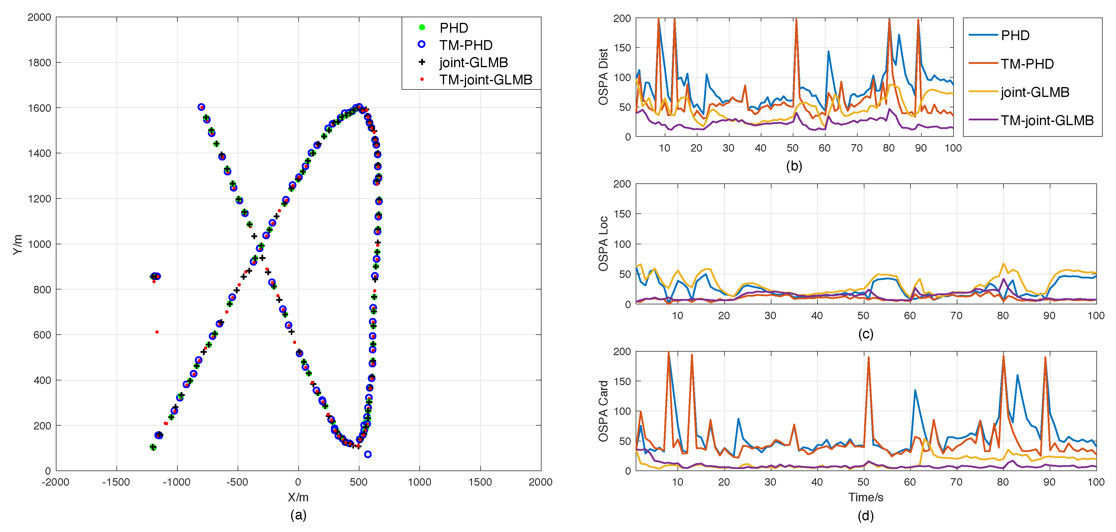
4.3. Result Analysis of Scenario 1
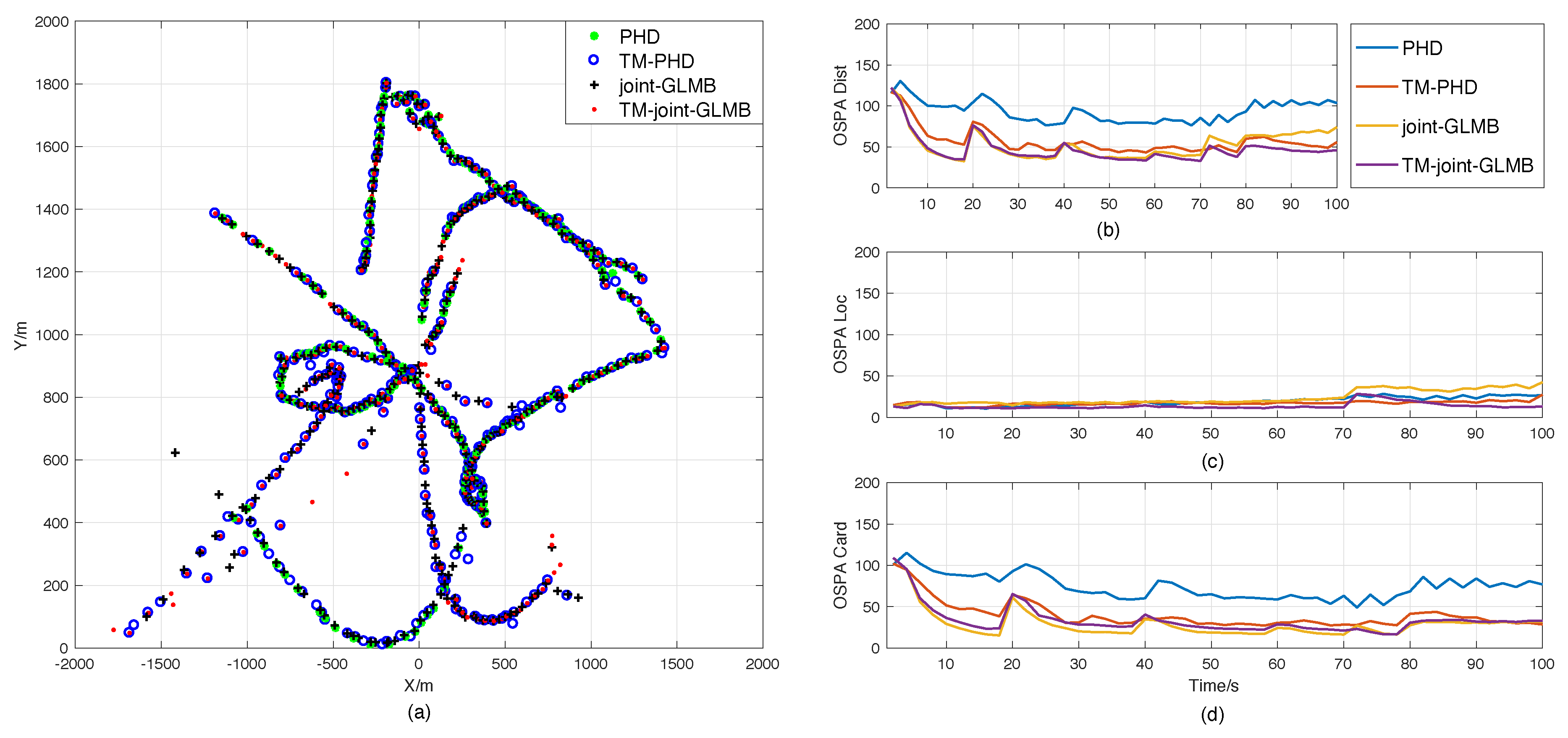
4.4. Result Analysis of Scenario 2
4.5. Result Analysis of Scenarios 3 and 4
5. Conclusions
Author Contributions
Acknowledgments
Conflicts of Interest
References
- Merrill, I.S. Introduction to Radar Systems; McGraw-Hill: New York, NY, USA, 2002. [Google Scholar]
- Tait, P. Introduction to Radar Target Recognition; IET: London, UK, 2009. [Google Scholar]
- Pace, P.E. Detecting and Classifying Low Probability of Intercept Radar; Artech House: Norwood, MA, USA, 2009. [Google Scholar]
- Gao, Y.; Jiang, D.; Liu, M. Wideband transmit beamforming using integer-time-delayed and phase-shifted waveforms. Electron. Lett. 2017, 53, 376–378. [Google Scholar] [CrossRef]
- Fu, W.; Jiang, D.; Su, Y.; Qian, R.; Gao, Y. Implementation of wideband digital transmitting beamformer based on LFM waveforms. IET Signal Process. 2017, 11, 205–212. [Google Scholar] [CrossRef]
- Curlander, J.C.; McDonough, R.N. Synthetic Aperture Radar; John Wiley & Sons: New York, NY, USA, 1991. [Google Scholar]
- Bar-Shalom, Y.; Willett, P.K.; Tian, X. Tracking and Data Fusion: A Handbook of Algorithms; YBS Publishing: Storrs, CT, USA, 2011. [Google Scholar]
- Blackman, S.; Popoli, R. Design and Analysis of Modern Tracking Systems; Artech House: Norwood, MA, USA, 1999. [Google Scholar]
- Challa, S.; Morelande, M.; Mušicki, D. Fundamentals of Object Tracking; Cambridge University Press: Cambridge, UK, 2011. [Google Scholar]
- Moller, J.; Waagepetersen, R.P. Modern statistics for spatial point processes. Scand. J. Stat. 2007, 34, 643–684. [Google Scholar] [CrossRef]
- Mahler, R.P.S. Advances in Statistical Multisource-Multitarget Information Fusion; Artech House: Norwood, MA, USA, 2014. [Google Scholar]
- Waller, L.A.; Gotway, C.A. Applied Spatial Statistics for Public Health Data; Wiley: New York, NY, USA, 2004. [Google Scholar]
- Mullane, J.; Vo, B.N.; Adams, M.D.; Vo, B.T. A random-finite-set approach to Bayesian SLAM. IEEE Trans. Robot. 2011, 27, 268–282. [Google Scholar] [CrossRef]
- Mullane, J.; Vo, B.N.; Adams, M.; Vo, B.T. Random Finite Sets in Robotic Map Building and SLAM; Springer: New York, NY, USA, 2011. [Google Scholar]
- Granström, K.; Lundquist, C.; Gustafsson, F.; Orguner, U. Random set methods: Estimation of multiple extended objects. IEEE Robot. Autom. Mag. 2014, 21, 73–82. [Google Scholar] [CrossRef]
- Blackman, S. Multiple hypothesis tracking for multiple target tracking. IEEE Aerosp. Electron. Syst. Mag. 2004, 19, 5–18. [Google Scholar] [CrossRef]
- Fortmann, T.; Bar-Shalom, Y.; Scheffe, M. Sonar tracking of multiple targets using joint probabilistic data association. IEEE J. Ocean. Eng. 1983, 8, 173–184. [Google Scholar] [CrossRef]
- Mahler, R.P.S. Multitarget bayes filtering via first-order multitarget moments. IEEE Trans. Aerosp. Electron. Syst. 2004, 39, 1152–1178. [Google Scholar] [CrossRef]
- Vo, B.T.; Vo, B.N.; Cantoni, A. Bayesian Filtering With Random Finite Set Observations. IEEE Trans. Signal Process. 2008, 56, 1313–1326. [Google Scholar] [CrossRef]
- Mahler, R.P.S. Statistical Multisource-Multitarget Information Fusion; Artech House: Norwood, MA, USA, 2007. [Google Scholar]
- Vo, B.T.; Vo, B.N.; Cantoni, A. Analytic implementations of the cardinalized probability hypothesis density filter. IEEE Trans. Signal Process. 2007, 55, 3553–3567. [Google Scholar] [CrossRef]
- Gao, Y.; Jiang, D.; Liu, M. Particle-gating SMC-PHD filter. Signal Process. 2017, 130, 64–73. [Google Scholar] [CrossRef]
- Liu, Z.; Chen, S.; Wu, H.; He, R.; Hao, L. A Student’st Mixture Probability Hypothesis Density Filter for Multi-Target Tracking with Outliers. Sensors 2018, 18, 1095. [Google Scholar] [CrossRef] [PubMed]
- Lian, F.; Hou, L.; Liu, J.; Han, C. Constrained Multi-Sensor Control Using a Multi-Target MSE Bound and a δ-GLMB Filter. Sensors 2018, 18, 2308. [Google Scholar] [CrossRef] [PubMed]
- Wei, B.; Nener, B. Distributed Space Debris Tracking with Consensus Labeled Random Finite Set Filtering. Sensors 2018, 18, 3005. [Google Scholar] [CrossRef] [PubMed]
- Mahler, R.P.S. PHD Filters of Higher Order in Target Number. IEEE Trans. Aerosp. Electron. Syst. 2007, 43, 1523–1543. [Google Scholar] [CrossRef]
- Vo, B.T.; Vo, B.N.; Cantoni, A. The Cardinality Balanced Multi-Target Multi-Bernoulli Filter and its Implementations. IEEE Trans. Signal Process. 2009, 57, 409–423. [Google Scholar] [CrossRef]
- Vo, B.T.; Vo, B.N. Labeled Random Finite Sets and Multi-Object Conjugate Priors. IEEE Trans. Signal Process. 2013, 61, 3460–3475. [Google Scholar] [CrossRef]
- Reuter, S.; Vo, B.T.; Vo, B.N.; Dietmayer, K. The Labeled Multi-Bernoulli Filter. IEEE Trans. Signal Process. 2014, 62, 3246–3260. [Google Scholar] [CrossRef]
- Vo, B.N.; Vo, B.T.; Phung, D. Labeled random finite sets and the Bayes multi-target tracking filter. IEEE Trans. Signal Process. 2014, 62, 6554–6567. [Google Scholar] [CrossRef]
- Beard, M.; Reuter, S.; Granström, K.; Vo, B.T.; Vo, B.N.; Scheel, A. Multiple extended target tracking with labeled random finite sets. IEEE Trans. Signal Process. 2016, 64, 1638–1653. [Google Scholar] [CrossRef]
- Vo, B.N.; Vo, B.T.; Hoang, H.G. An efficient implementation of the generalized labeled multi-Bernoulli filter. IEEE Trans. Signal Process. 2017, 65, 1975–1987. [Google Scholar] [CrossRef]
- Vo, B.N.; Singh, S.; Doucet, A. Sequential Monte Carlo Methods for Multitarget Filtering with Random Finite Sets. IEEE Trans. Aerosp. Electron. Syst. 2005, 41, 1224–1245. [Google Scholar] [CrossRef]
- Vo, B.N.; Ma, W.K. The Gaussian Mixture Probability Hypothesis Density Filter. IEEE Trans. Signal Process. 2006, 54, 4091–4104. [Google Scholar] [CrossRef]
- Macagnano, D.; De Abreu, G.T.F. Adaptive gating for multitarget tracking with Gaussian mixture filters. IEEE Trans. Signal Process. 2012, 60, 1533–1538. [Google Scholar] [CrossRef]
- Li, T.; Sun, S.; Sattar, T.P. High-speed Sigma-gating SMC-PHD filter. Signal Process. 2013, 93, 2586–2593. [Google Scholar] [CrossRef]
- Koch, J.W. Bayesian approach to extended object and cluster tracking using random matrices. IEEE Trans. Aerosp. Electron. Syst. 2008, 44, 1042–1059. [Google Scholar] [CrossRef]
- Schuhmacher, D.; Vo, B.T.; Vo, B.N. A Consistent Metric for Performance Evaluation of Multi-Object Filters. IEEE Trans. Signal Process. 2008, 56, 3447–3457. [Google Scholar] [CrossRef]


| Sector No. | 1 | 2 | 3 | 4 | 5 | 6 | 7 | 8 | 9 | 10 |
| Left border | ||||||||||
| Right border | ||||||||||
| Scanning order | 1 | 3 | 5 | 7 | 9 | 11 | 13 | 15 | 17 | 19 |
| Sector No. | 11 | 12 | 13 | 14 | 15 | 16 | 17 | 18 | 19 | 20 |
| Left border | ||||||||||
| Right border | ||||||||||
| Scanning order | 2 | 4 | 6 | 8 | 10 | 12 | 14 | 16 | 18 | 20 |
| Target Index | Lifetime (s) | Initial States (m, m/s, m/s, m, m/s, m/s) |
|---|---|---|
| # 1 | ||
| # 2 | ||
| # 3 | ||
| # 4 | ||
| # 5 | ||
| # 6 | ||
| # 7 | ||
| # 8 | ||
| # 9 | ||
| # 10 | ||
| # 11 | ||
| # 12 |
© 2018 by the authors. Licensee MDPI, Basel, Switzerland. This article is an open access article distributed under the terms and conditions of the Creative Commons Attribution (CC BY) license (http://creativecommons.org/licenses/by/4.0/).
Share and Cite
Jiang, D.; Liu, M.; Gao, Y.; Gao, Y.; Fu, W.; Han, Y. Time-Matching Random Finite Set-Based Filter for Radar Multi-Target Tracking. Sensors 2018, 18, 4416. https://doi.org/10.3390/s18124416
Jiang D, Liu M, Gao Y, Gao Y, Fu W, Han Y. Time-Matching Random Finite Set-Based Filter for Radar Multi-Target Tracking. Sensors. 2018; 18(12):4416. https://doi.org/10.3390/s18124416
Chicago/Turabian StyleJiang, Defu, Ming Liu, Yiyue Gao, Yang Gao, Wei Fu, and Yan Han. 2018. "Time-Matching Random Finite Set-Based Filter for Radar Multi-Target Tracking" Sensors 18, no. 12: 4416. https://doi.org/10.3390/s18124416
APA StyleJiang, D., Liu, M., Gao, Y., Gao, Y., Fu, W., & Han, Y. (2018). Time-Matching Random Finite Set-Based Filter for Radar Multi-Target Tracking. Sensors, 18(12), 4416. https://doi.org/10.3390/s18124416