IMU-to-Segment Assignment and Orientation Alignment for the Lower Body Using Deep Learning


Abstract
:1. Introduction
1.1. I2S Assignment and Alignment for Inertial Body Motion Capture
1.2. I2S Assignment and Alignment for Activity Recognition, Deep Learning Approaches
1.3. Applications with Simulated/Synthetic IMU Data
1.4. Contributions and Scope
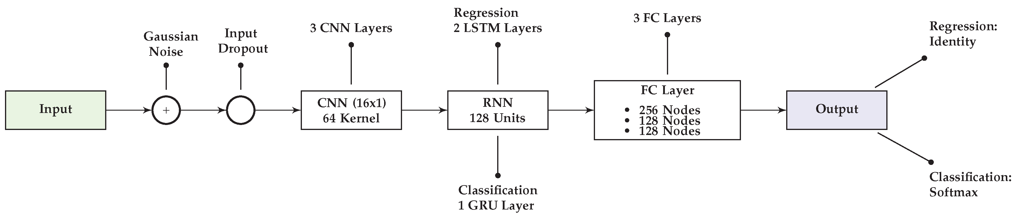
- We propose real-time capable deep learning approaches to solve the I2S assignment problem via classification and the I2S alignment problem via regression during walking for IMUs mounted on the lower body. The proposed approaches combine automatic feature learning via CNN units with time dynamic features based on two recurrent neural network approaches (LSTM and GRU). Since each IMU is handled individually, the proposed approaches scale to an arbitrary number of IMUs.
- We propose and evaluate methods for simulating IMU training data for a variety of I2S alignment orientations during walking using freely available [49] and newly recorded motion capture datasets. This is our approach for counteracting the problem of requiring the recording of exponentially many training data for sufficiently sampling potential I2S alignment variations.
- We investigate the performances of the proposed methods and approaches on simulated and real IMU test data, with different proportions of simulated and real IMU data used for training. The experiments show promising performances for both the classification and the regression problem with only a small amount of recorded IMU data (in terms of alignment variations).
2. Methods
2.1. Problem Statement
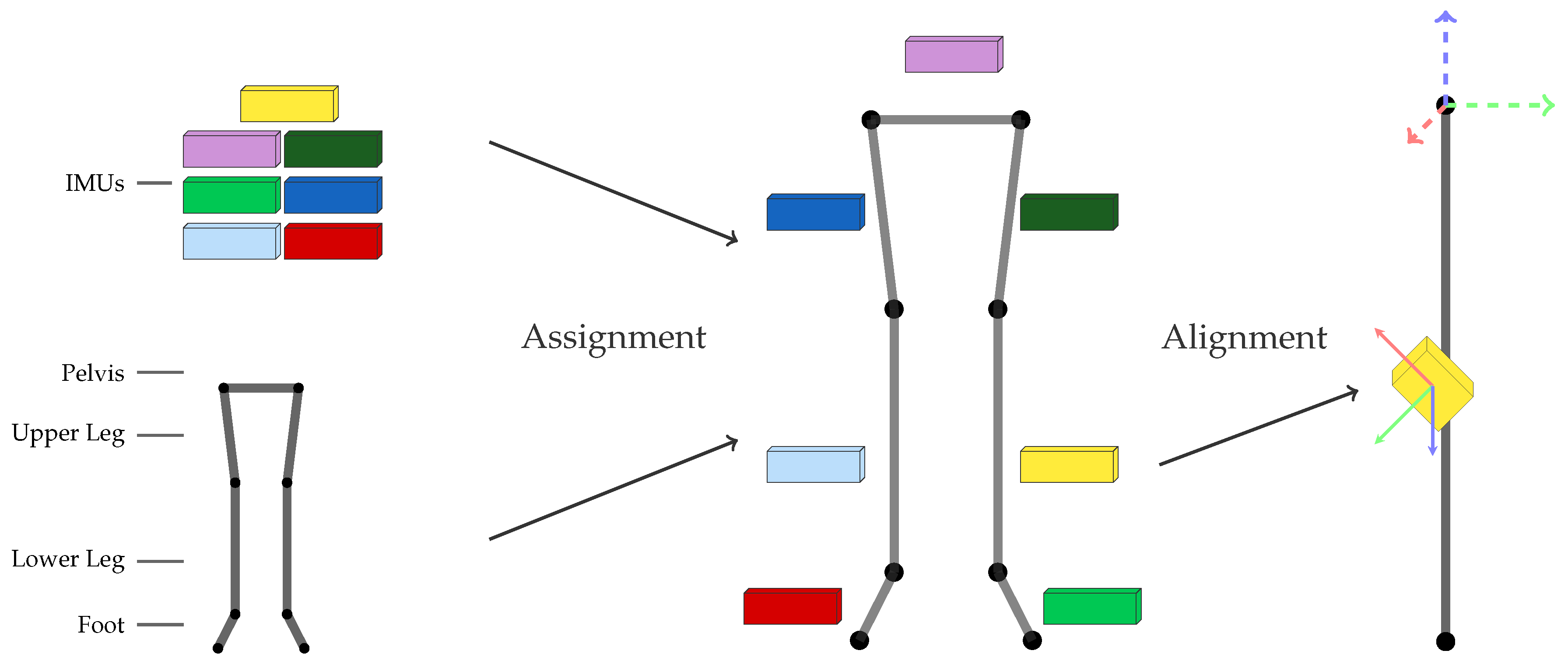
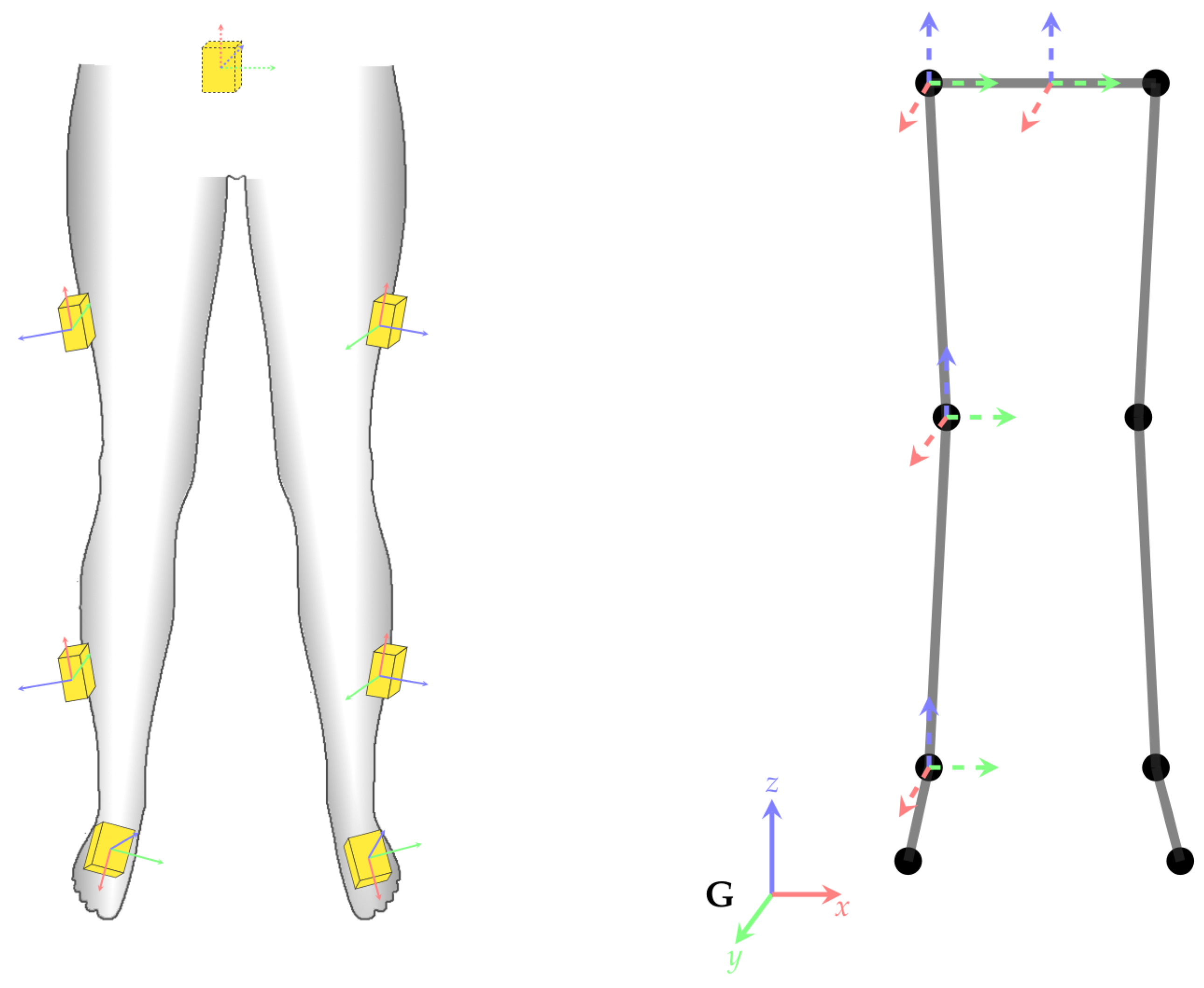
- I2S assignment: Each IMU is separately assigned to the skeleton segment it is attached to. This results in the classification problem of mapping a window of (raw) IMU data to one of the seven classes associated to the lower body segments: (1) LeftFoot; (2) LeftLowerLeg; (3) LeftUpperLeg; (4) Pelvis; (5) RightUpperLeg; (6) RightLowerLeg; and (7) RightFoot.
- I2S alignment: Each IMU’s orientation w.r.t. the associated segment is estimated via regression based on a window of IMU data. Note, I2S positions are assumed constant (on the middle of the respective segment) in this work.
2.2. Proposed Networks
2.2.1. Notation
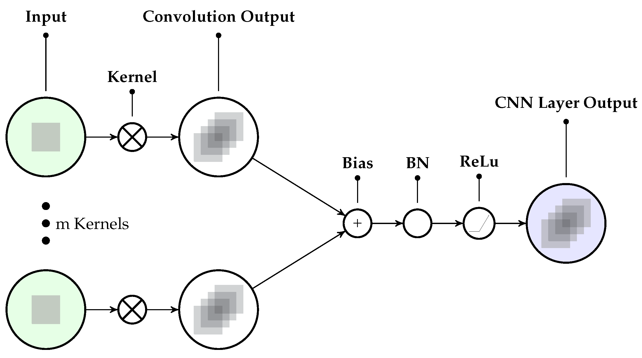
2.2.2. Convolutional Neural Network (CNN) Layer
2.2.3. Recurrent Neural Network (RNN) Layer
2.2.4. Dropout Layer
2.2.5. Application of the Proposed Networks
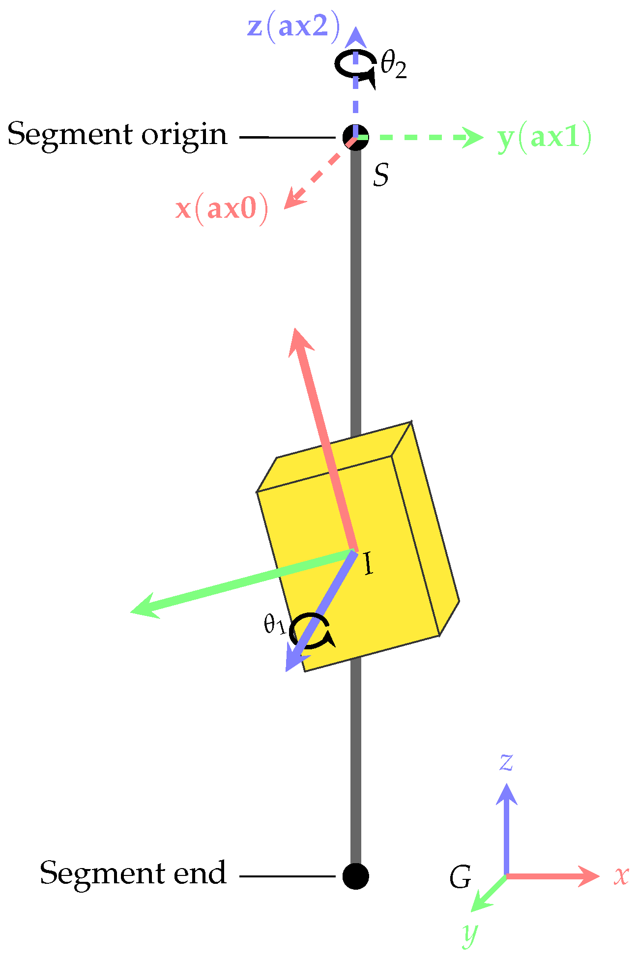
2.3. Coordinate frames and transformations
2.4. Creation of Artificial Training Data
2.4.1. Simulation of I2S Alignment Variations
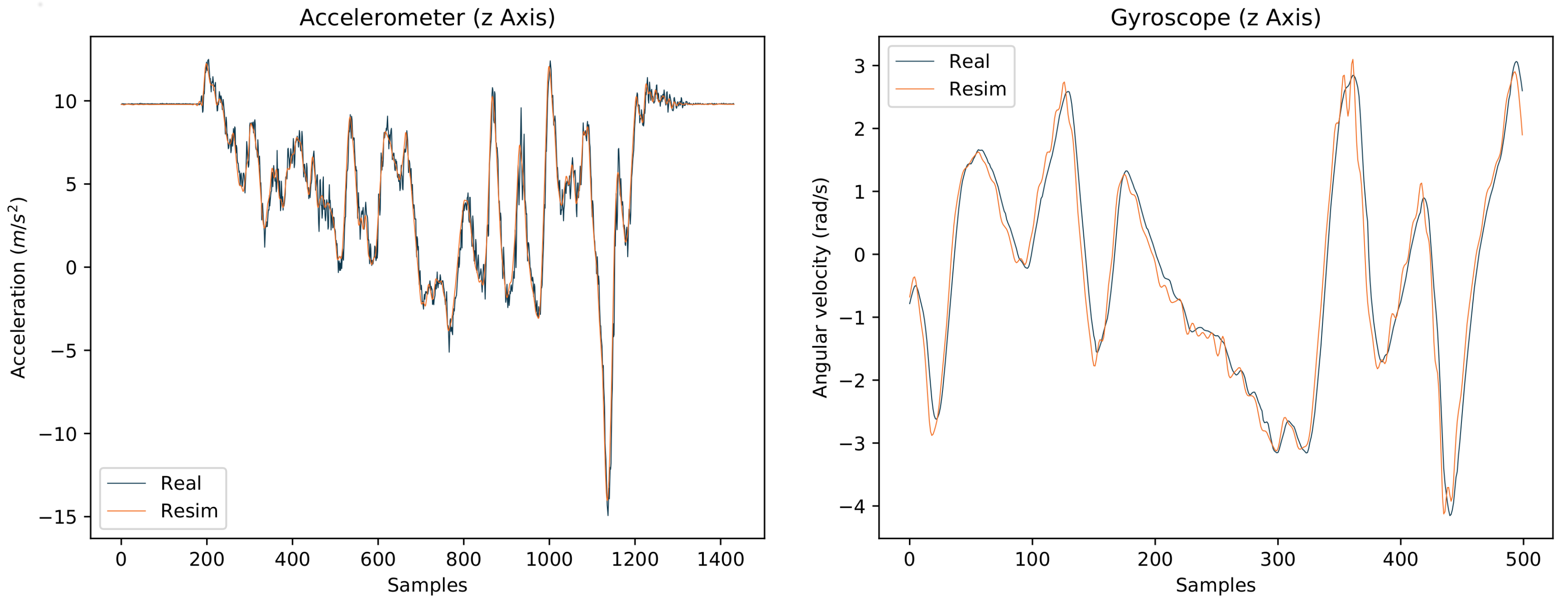
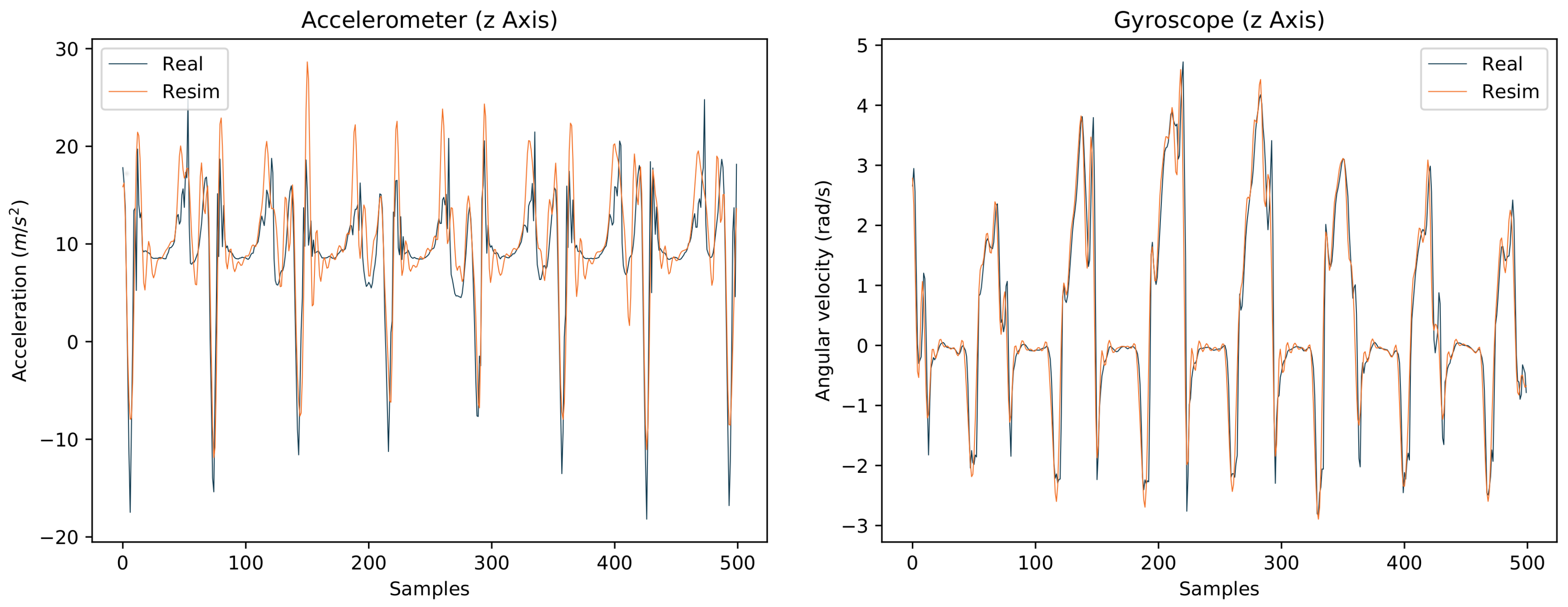
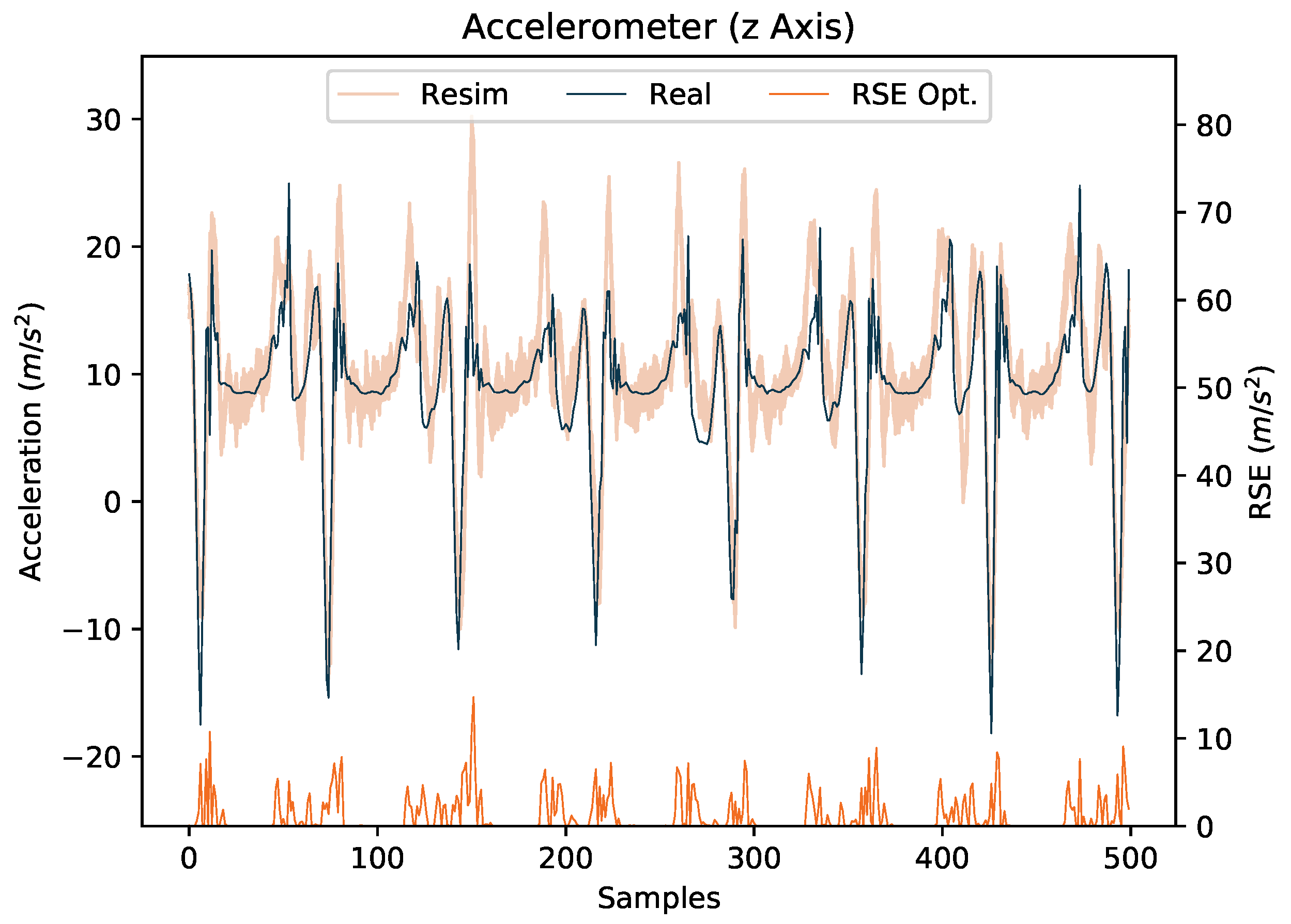
2.4.2. Simulation of Realistic IMU Data
3. Datasets and Experiments
3.1. Datasets
- A
- IMU data simulated from the 3D kinematics data of parts of the CMU dataset (42 participants performing different walking styles, see Table A6 in Appendix C). Note, this dataset is distinguished by a high amount of simulated IMU configuration variations (as described in Section 2.4) based on an already high amount of variability in the 3D kinematics data (in terms of persons and walking styles) used for simulation.
- B
- Collected real IMU data from four male participants (mean age: 32, mean weight: 82 kg, mean height: 181 cm) instructed to walk for one minute back and forth (within an area of five by five meters), with nine different IMU configurations as detailed in Appendix C (Table A7).
- C
- Collected real IMU data from 28 participants (13/15 male/female, mean age: 25 years, mean weight: 70 kg, mean height: 176 cm) instructed to walk for six minutes in an eight-shape within an area of about five by five meters, with one standard IMU configuration, different from the previously mentioned nine configurations (see Figure 8). This study was approved by the Ethical Committee of the University of Kaiserslautern and written informed consent was obtained from all participants prior to their participation.
3.2. Training
3.3. Evaluation
4. Results and Discussion
4.1. Evaluation of Network Configurations on Dataset A
4.2. Pre-trained Models Based on Dataset A
4.3. Impact of Mixing Real and Simulated IMU Training Data Based on Dataset B
- Training on real IMU data from three persons (nine alignment variations each, see Table A7 in Appendix C), testing on real IMU data from the left out (test) person (nine alignment variations).
- Training on re-simulated IMU data from three persons (64 simulated alignment variations per real IMU alignment), testing on real IMU data from the test person (nine alignment variations).
- Setup 2, but with additionally using the real IMU data captured from the three participants (nine alignment variations) for training (i.e., of the training data is based on real IMU data).
- Setup 3, with the training being warm-started with the pre-trained models of Section 4.2.
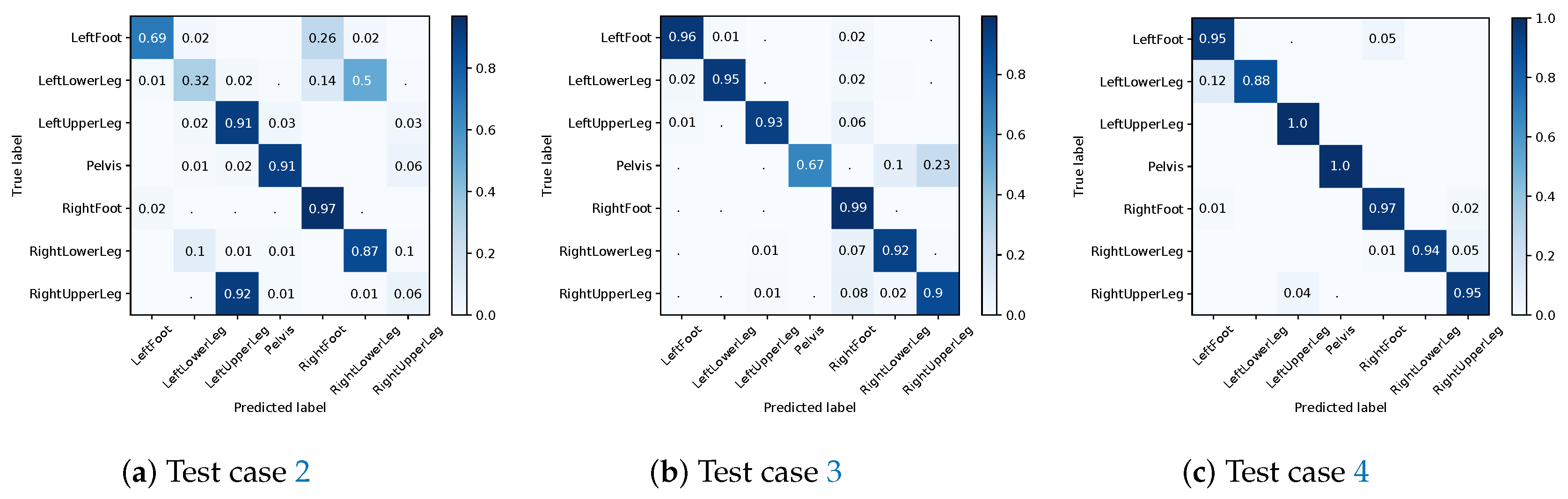
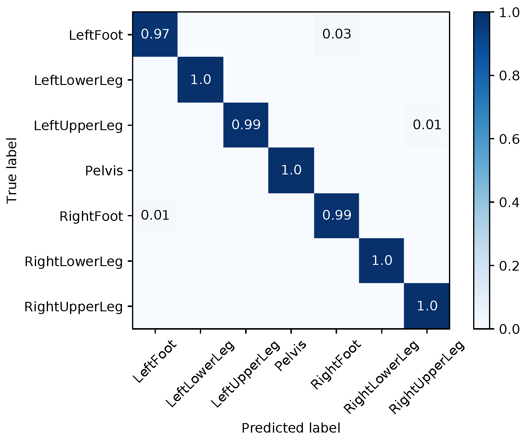
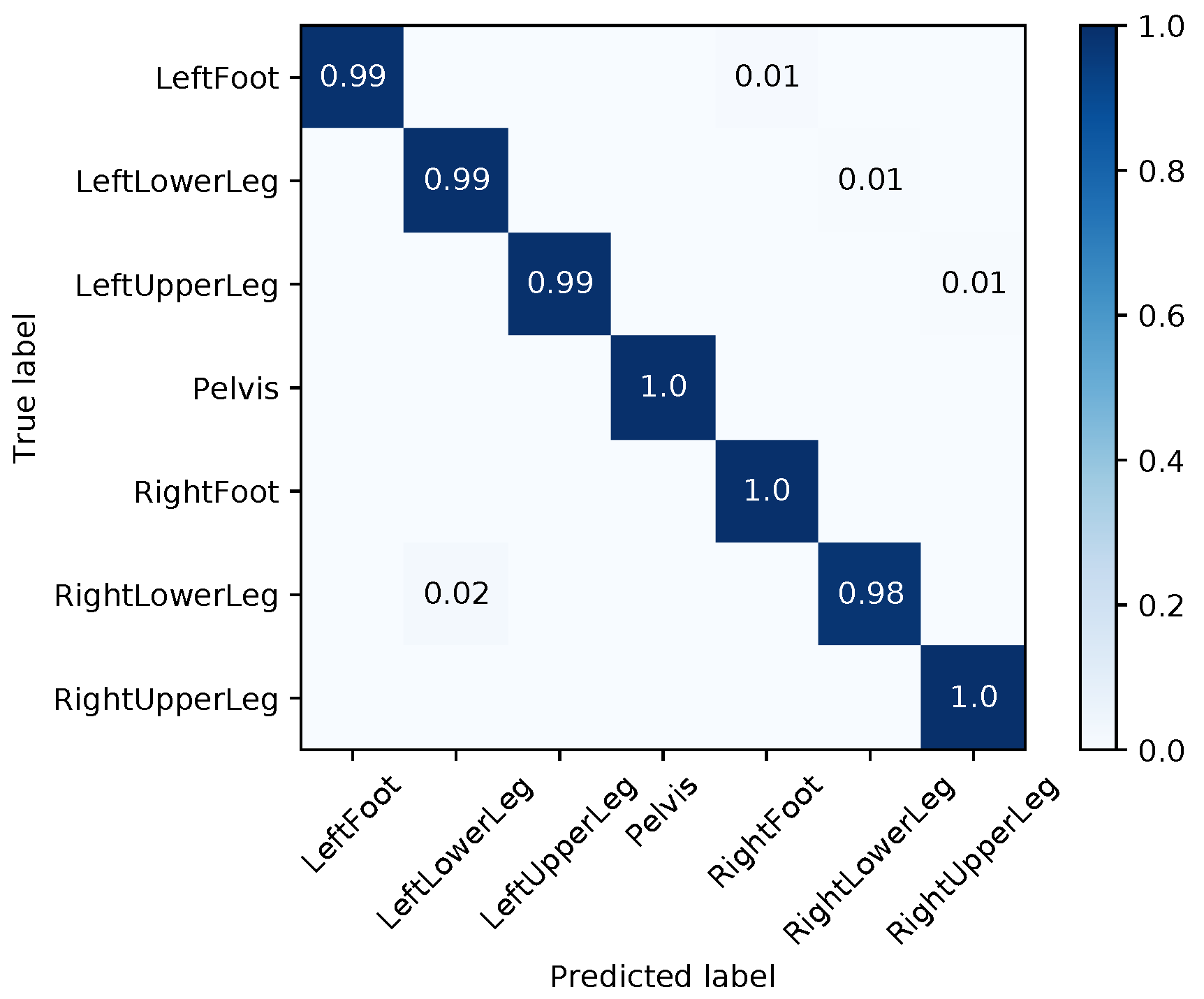
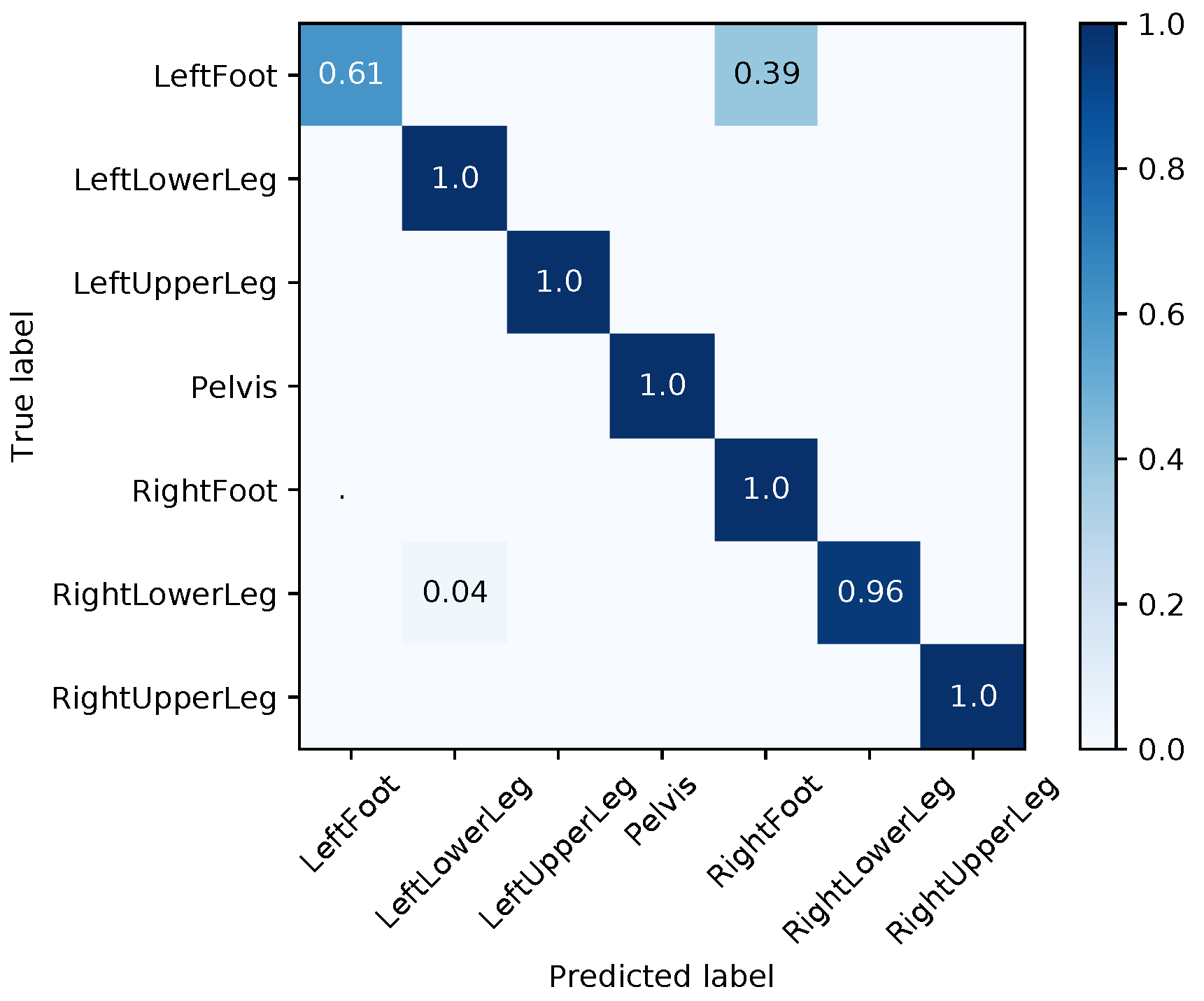
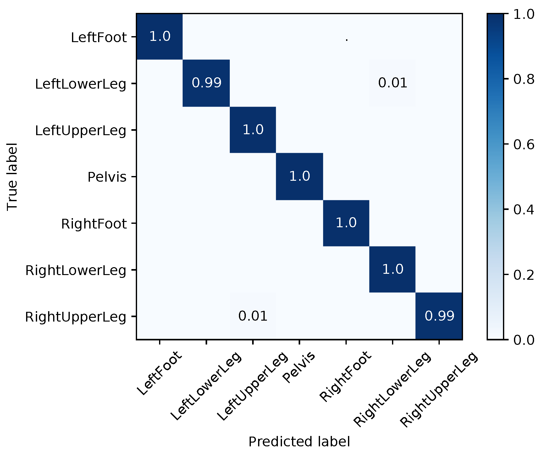
4.3.1. I2S Assignment Problem
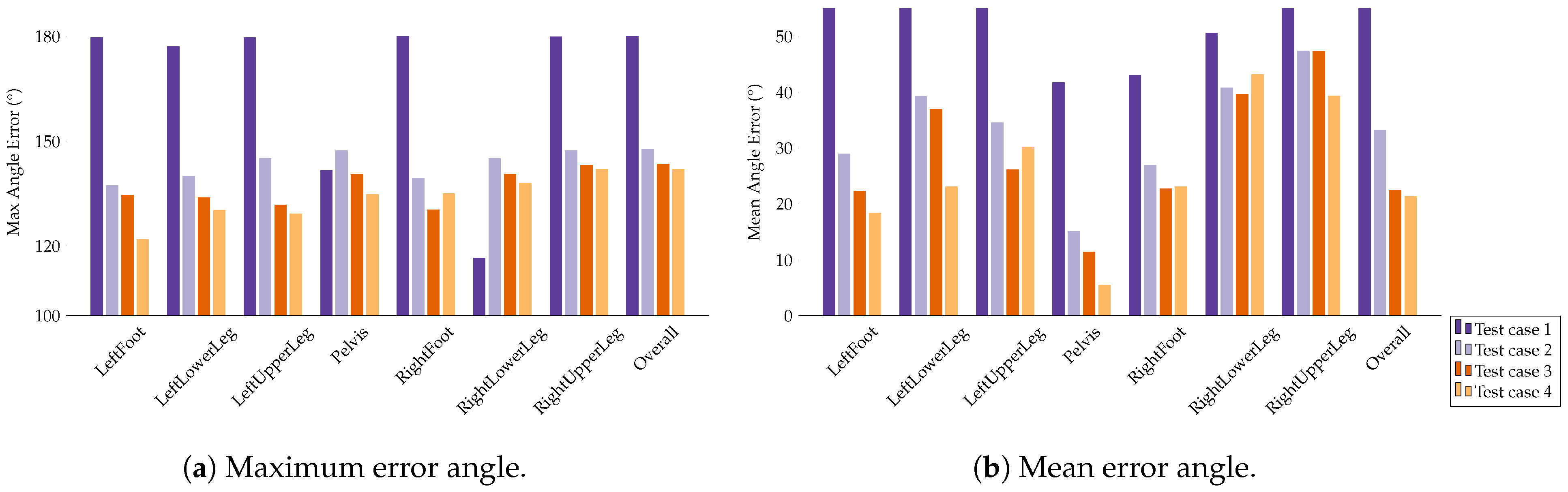
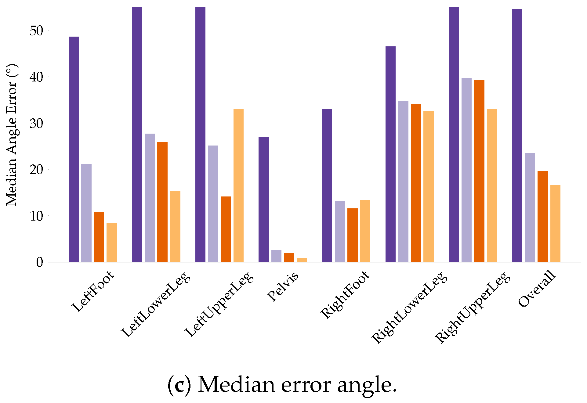
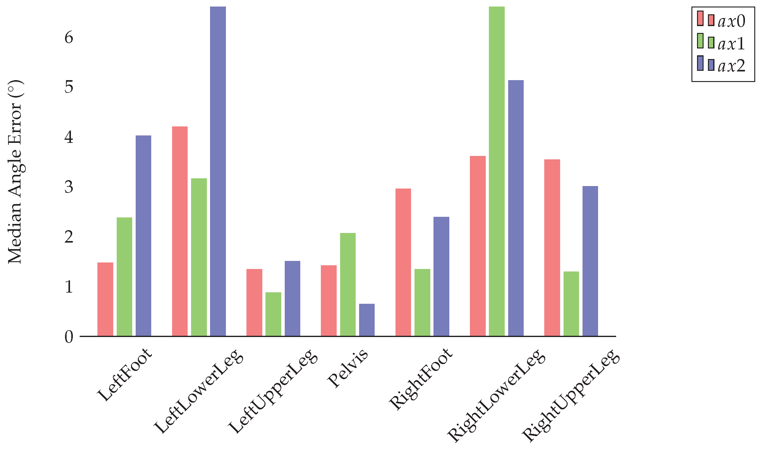
4.3.2. I2S Alignment Problem
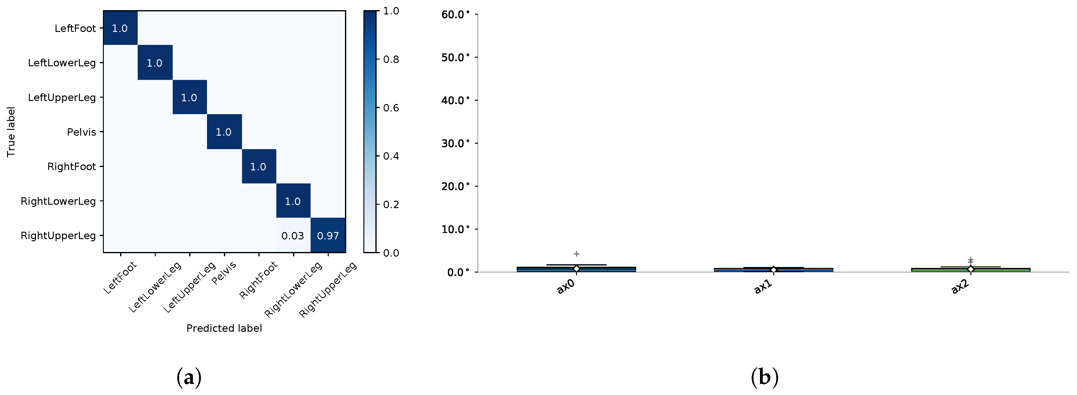
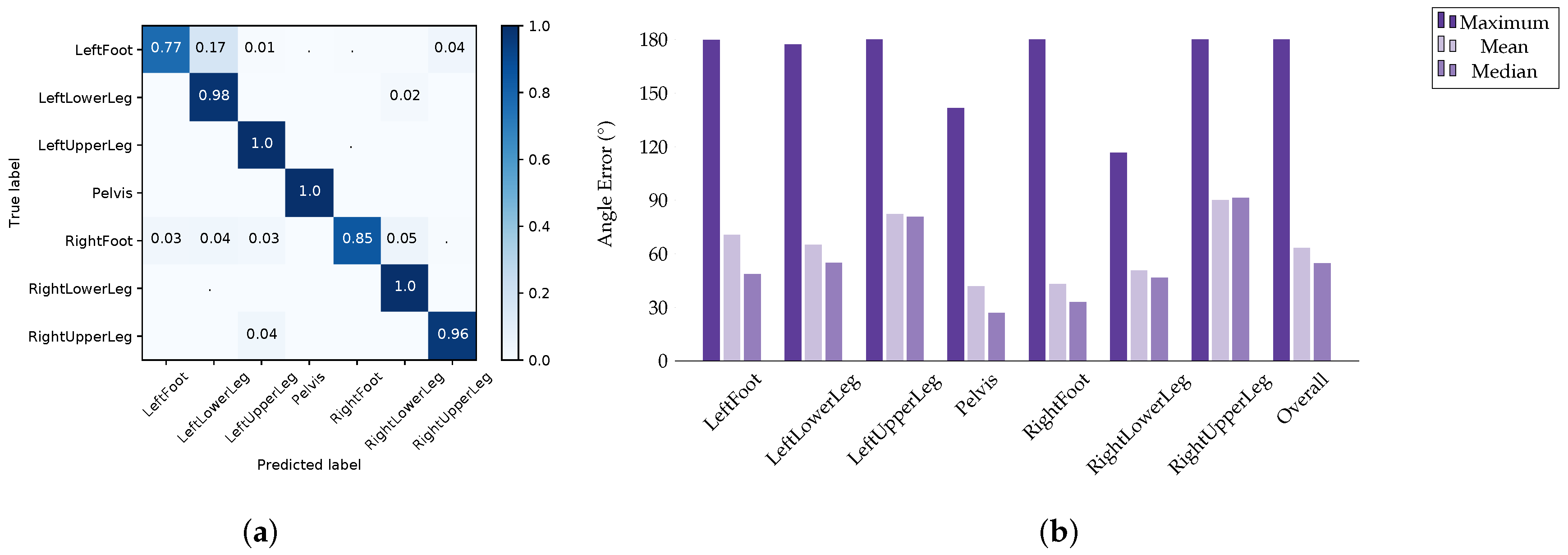
4.4. Evaluation of the Final Models
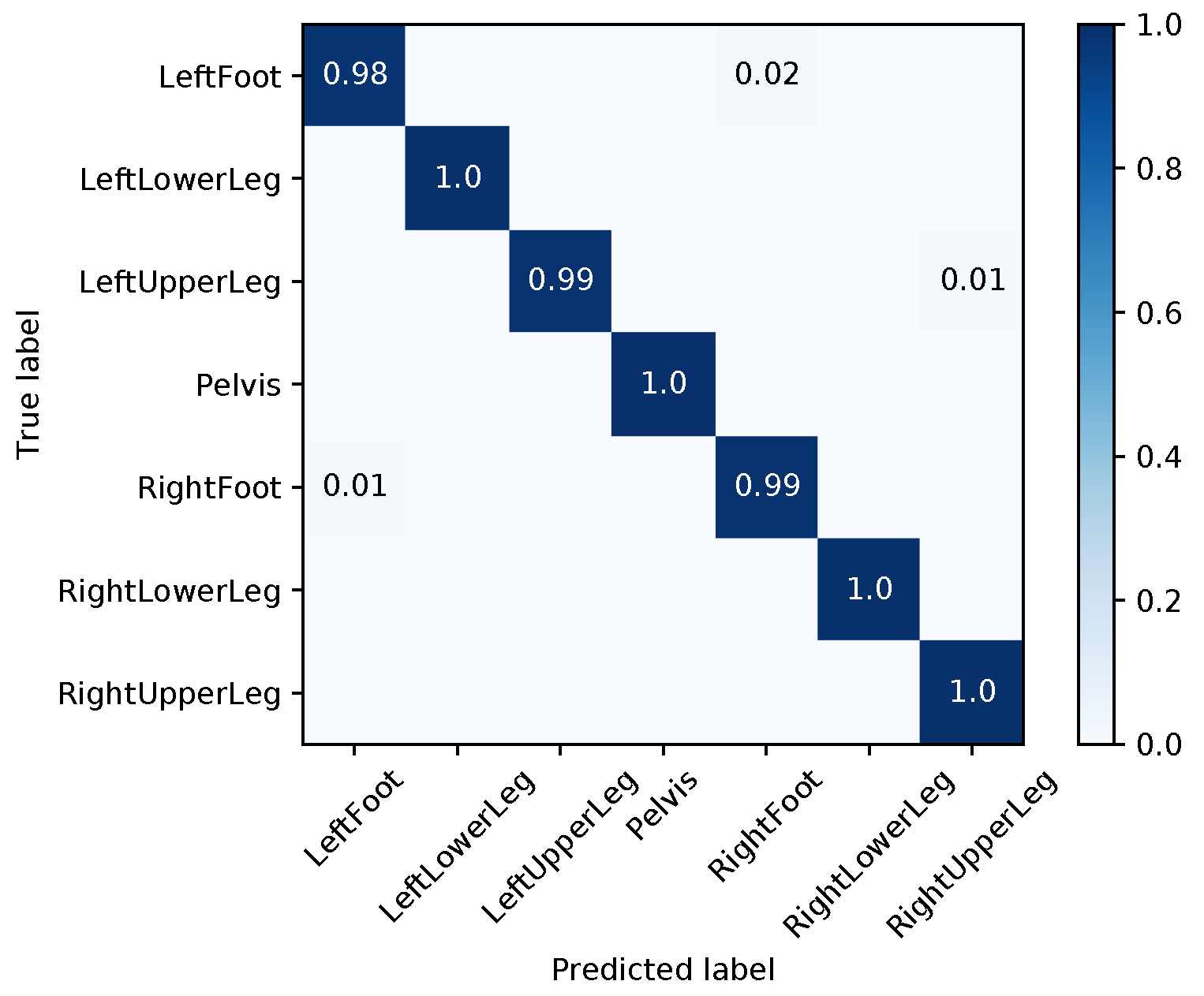
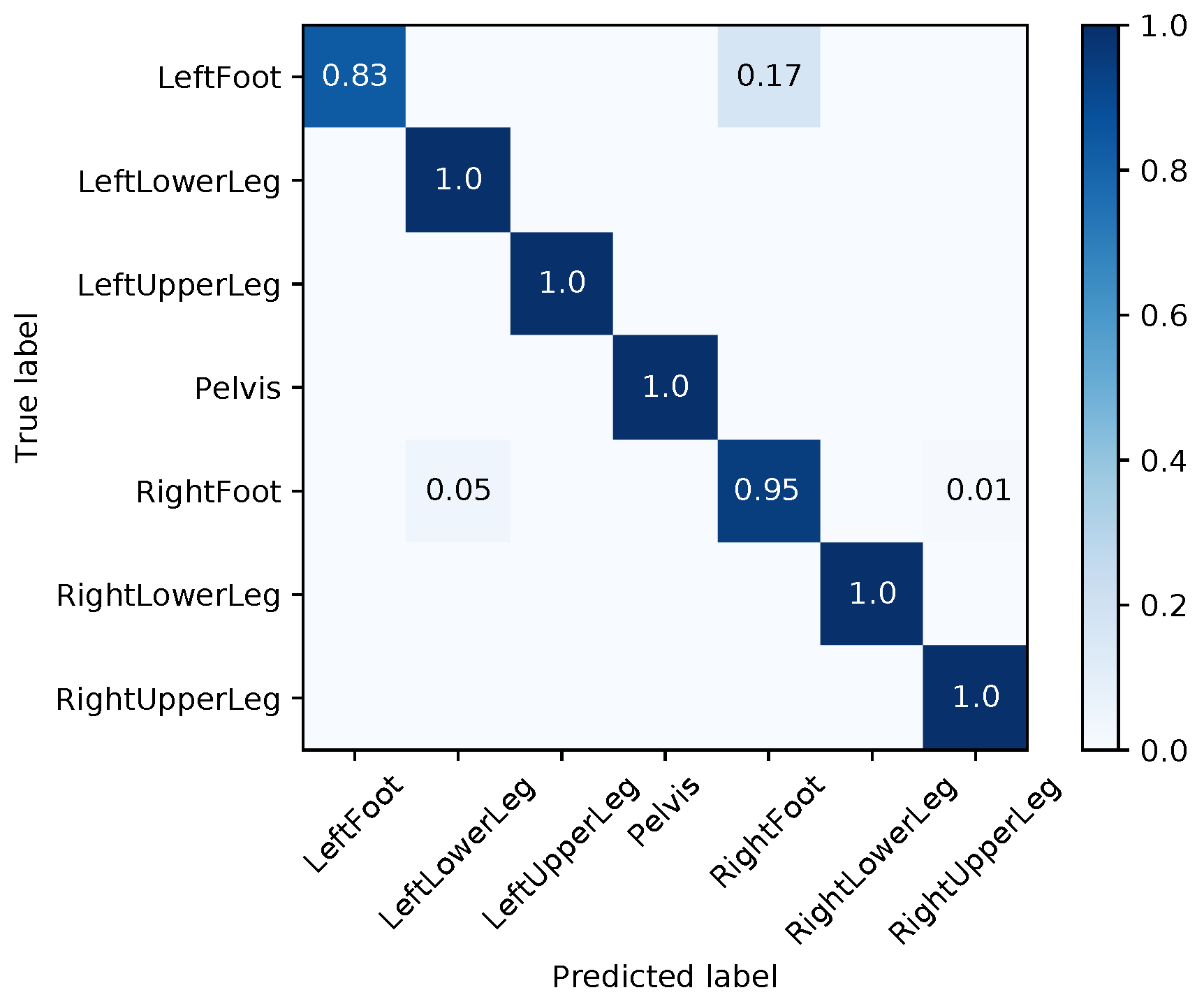
4.4.1. I2S Assignment Problem
4.4.2. I2S Alignment Problem
5. Conclusions
Acknowledgments
Author Contributions
Conflicts of Interest
Appendix A. Proposed Network Configurations
Appendix A.1. Long Short-Term Memory (LSTM)
Appendix A.2. Gated Recurrent Unit (GRU)
Appendix A.3. Hyper Parameters

| Assignment | Alignment | ||
|---|---|---|---|
| Optimizer | Batch size | 256 | 256 |
| Learning rate | 0.001 | 0.001 | |
| Optimizer | Adam | Adam | |
| CNN Layer | # Layer | 3 | 3 |
| Kernel | 16 × 1 | 16 × 1 | |
| # Kernel | 64 | 64 | |
| RNN Layer | # Layer | 1 | 2 |
| Cell | GRU | LSTM | |
| # Units | 128 | 128 | |
| Regularization | -Factor | 0.0001 | 0.0001 |
| Keep probability | 0.8 | 0.8 |
Appendix B. IMU Data Simulation
| Accelerometer (Pearson Correlation Coefficient) | ||||
| IMU | mean | |||
| 1 | 0.9903 | 0.9915 | 0.9862 | 0.9893 |
| 2 | 0.9901 | 0.9898 | 0.9819 | 0.9873 |
| 3 | 0.9913 | 0.9909 | 0.9854 | 0.9892 |
| 4 | 0.9918 | 0.9828 | 0.9762 | 0.9836 |
| 5 | 0.9917 | 0.9875 | 0.9819 | 0.9870 |
| 6 | 0.9897 | 0.9869 | 0.9756 | 0.9841 |
| 7 | 0.9908 | 0.9920 | 0.9866 | 0.9898 |
| mean | 0.9908 | 0.9888 | 0.9820 | 0.9872 |
| Accelerometer RMSE [m/s] | ||||
| mean | ||||
| 1 | 0.6950 | 0.6969 | 0.7934 | 0.7285 |
| 2 | 0.7190 | 0.7977 | 0.9613 | 0.8260 |
| 3 | 0.6506 | 0.6991 | 0.7894 | 0.7130 |
| 4 | 0.6814 | 0.9577 | 1.0750 | 0.9047 |
| 5 | 0.6640 | 0.8111 | 0.9024 | 0.7925 |
| 6 | 0.7534 | 0.9265 | 1.2443 | 0.9747 |
| 7 | 0.6869 | 0.6644 | 0.7574 | 0.7029 |
| mean | 0.6929 | 0.7933 | 0.9319 | 0.8060 |
| Gyroscope (Pearson Correlation Coefficient) | ||||
| IMU | mean | |||
| 1 | 0.9594 | 0.9760 | 0.9778 | 0.9711 |
| 2 | 0.9637 | 0.9793 | 0.9737 | 0.9722 |
| 3 | 0.9645 | 0.9800 | 0.9759 | 0.9734 |
| 4 | 0.9617 | 0.9798 | 0.9753 | 0.9723 |
| 5 | 0.9640 | 0.9798 | 0.9750 | 0.9729 |
| 6 | 0.9632 | 0.9816 | 0.9776 | 0.9742 |
| 7 | 0.9652 | 0.9800 | 0.9766 | 0.9739 |
| mean | 0.9631 | 0.9795 | 0.9760 | 0.9729 |
| Gyroscope RMSE [rad/s] | ||||
| IMU | mean | |||
| 1 | 0.5978 | 0.3519 | 0.2661 | 0.4053 |
| 2 | 0.5671 | 0.3252 | 0.2904 | 0.3942 |
| 3 | 0.5604 | 0.3210 | 0.2782 | 0.3865 |
| 4 | 0.5840 | 0.3236 | 0.2811 | 0.3962 |
| 5 | 0.5636 | 0.3231 | 0.2834 | 0.3901 |
| 6 | 0.5838 | 0.3060 | 0.2700 | 0.3866 |
| 7 | 0.5558 | 0.3193 | 0.2745 | 0.3832 |
| mean | 0.5732 | 0.3243 | 0.2777 | 0.3917 |
| Accelerometer (Pearson Correlation Coefficient) | ||||
| IMU | mean | |||
| LeftLowerLeg | 0.7428 | 0.4830 | 0.6028 | 0.6095 |
| RightUpperLeg | 0.5726 | 0.2803 | 0.7139 | 0.5223 |
| LeftUpperLeg | 0.6717 | 0.1602 | 0.7737 | 0.5352 |
| RightLowerLeg | 0.7325 | 0.3326 | 0.5148 | 0.5266 |
| LeftFoot | 0.8067 | 0.3962 | 0.6565 | 0.6198 |
| Pelvis | 0.8132 | 0.2409 | 0.4940 | 0.5161 |
| RightFoot | 0.8456 | 0.4342 | 0.8026 | 0.6942 |
| mean | 0.7407 | 0.3325 | 0.6512 | 0.5748 |
| Accelerometer RMSE [m/s] | ||||
| IMU | mean | |||
| LeftLowerLeg | 3.6462 | 4.3371 | 4.1111 | 4.0314 |
| RightUpperLeg | 4.2053 | 3.2582 | 3.8274 | 3.7637 |
| LeftUpperLeg | 3.1212 | 3.9498 | 3.4068 | 3.4926 |
| RightLowerLeg | 3.9041 | 5.0482 | 4.3344 | 4.4289 |
| LeftFoot | 5.3138 | 4.9329 | 4.7109 | 4.9859 |
| Pelvis | 2.2677 | 2.5007 | 2.3478 | 2.3720 |
| RightFoot | 4.6748 | 6.4197 | 4.0363 | 5.0436 |
| mean | 3.8762 | 4.3495 | 3.8250 | 4.0169 |
| Gyroscope (Pearson Correlation Coefficient) | ||||
| IMU | mean | |||
| LeftLowerLeg | 0.8720 | 0.9802 | 0.9628 | 0.9383 |
| RightUpperLeg | 0.8736 | 0.9570 | 0.9207 | 0.9171 |
| LeftUpperLeg | 0.8661 | 0.9692 | 0.8901 | 0.9085 |
| RightLowerLeg | 0.8681 | 0.9820 | 0.9469 | 0.9323 |
| LeftFoot | 0.9145 | 0.9618 | 0.9234 | 0.9332 |
| Pelvis | 0.9778 | 0.8890 | 0.9349 | 0.9339 |
| RightFoot | 0.8451 | 0.9673 | 0.9504 | 0.9209 |
| mean | 0.8882 | 0.9581 | 0.9327 | 0.9263 |
| Gyroscope RMSE [rad/s] | ||||
| IMU | mean | |||
| LeftLowerLeg | 0.8678 | 0.5459 | 0.2285 | 0.5474 |
| RightUpperLeg | 0.6663 | 0.4652 | 0.1804 | 0.4373 |
| LeftUpperLeg | 0.8404 | 0.3579 | 0.2251 | 0.4745 |
| RightLowerLeg | 0.7338 | 0.5556 | 0.1653 | 0.4849 |
| LeftFoot | 0.6386 | 1.0709 | 0.4129 | 0.7075 |
| Pelvis | 0.1287 | 0.1257 | 0.0938 | 0.1161 |
| RightFoot | 0.4638 | 1.0177 | 0.4836 | 0.6550 |
| mean | 0.6199 | 0.5913 | 0.2557 | 0.4890 |
Appendix C. Datasets
| Participant ID | Recording | Frames | Duration [s] | Motion Description |
|---|---|---|---|---|
| 02 | 01 | 313 | 313. | Walk |
| 02 | 298 | 298. | Walk | |
| 03 | 01 | 432 | 432. | Walk on uneven terrain |
| 02 | 365 | 365. | Walk on uneven terrain | |
| 03 | 4563 | 4563. | Walk on uneven terrain | |
| 04 | 4722 | 4722. | Walk on uneven terrain | |
| 05 | 01 | 598 | 598. | Walk |
| 06 | 01 | 494 | 494. | Walk |
| 07 | 01 | 316 | 316. | Walk |
| 02 | 329 | 329. | Walk | |
| 03 | 415 | 415. | Walk | |
| 04 | 449 | 449. | Slow walk | |
| 05 | 517 | 517. | Slow walk | |
| 06 | 417 | 417. | Walk | |
| 07 | 379 | 379. | Walk | |
| 08 | 362 | 362. | Walk | |
| 09 | 306 | 306. | Walk | |
| 10 | 301 | 301. | Walk | |
| 11 | 315 | 315. | Walk | |
| 08 | 01 | 277 | 277. | Walk |
| 02 | 309 | 309. | Walk | |
| 03 | 353 | 353. | Walk | |
| 04 | 484 | 484. | Slow walk | |
| 06 | 296 | 296. | Walk | |
| 08 | 283 | 283. | Walk | |
| 09 | 293 | 293. | Walk | |
| 10 | 275 | 275. | Walk | |
| 10 | 04 | 549 | 549. | Walk |
| 12 | 01 | 523 | 523. | Walk |
| 02 | 673 | 673. | Walk | |
| 03 | 565 | 565. | Walk | |
| 15 | 01 | 5524 | 5524. | Walk / wander |
| 03 | 12550 | 12550. | Walk/wander | |
| 09 | 7875 | 7875. | Walk/wander | |
| 14 | 9003 | 9003. | Walk/wander | |
| 16 | 15 | 471 | 471. | Walk |
| 16 | 510 | 510. | Walk | |
| 21 | 312 | 312. | Walk | |
| 22 | 307 | 307. | Walk | |
| 31 | 424 | 424. | Walk | |
| 32 | 580 | 580. | Walk | |
| 47 | 416 | 416. | Walk | |
| 58 | 342 | 342. | Walk | |
| 26 | 01 | 833 | 833. | Walk |
| 27 | 01 | 1033 | 1033. | Walk |
| 29 | 01 | 1316 | 1316. | Walk |
| 32 | 01 | 482 | 482. | Walk |
| 02 | 434 | 434. | Walk | |
| 36 | 01 | 557 | 557. | Walk on uneven terrain |
| 04 | 3726 | 3726. | Walk on uneven terrain | |
| 05 | 4196 | 4196. | Walk on uneven terrain | |
| 06 | 3896 | 3896. | Walk on uneven terrain | |
| 07 | 3772 | 3772. | Walk on uneven terrain | |
| 08 | 3714 | 3714. | Walk on uneven terrain | |
| 10 | 3832 | 3832. | Walk on uneven terrain | |
| 11 | 4168 | 4168. | Walk on uneven terrain | |
| 12 | 4585 | 4585. | Walk on uneven terrain | |
| 13 | 4247 | 4247. | Walk on uneven terrain | |
| 14 | 4146 | 4146. | Walk on uneven terrain | |
| 15 | 4164 | 4164. | Walk on uneven terrain | |
| 16 | 4395 | 4395. | Walk on uneven terrain | |
| 17 | 4359 | 4359. | Walk on uneven terrain | |
| 18 | 4304 | 4304. | Walk on uneven terrain | |
| 19 | 4193 | 4193. | Walk on uneven terrain | |
| 20 | 4090 | 4090. | Walk on uneven terrain | |
| 21 | 4030 | 4030. | Walk on uneven terrain | |
| 22 | 4312 | 4312. | Walk on uneven terrain | |
| 23 | 4392 | 4392. | Walk on uneven terrain | |
| 24 | 4153 | 4153. | Walk on uneven terrain | |
| 25 | 4685 | 4685. | Walk on uneven terrain | |
| 26 | 4237 | 4237. | Walk on uneven terrain | |
| 27 | 4247 | 4247. | Walk on uneven terrain | |
| 28 | 2391 | 2391. | Walk on uneven terrain | |
| 29 | 4469 | 4469. | Walk on uneven terrain | |
| 30 | 4414 | 4414. | Walk on uneven terrain | |
| 31 | 3736 | 3736. | Walk on uneven terrain | |
| 32 | 4468 | 4468. | Walk on uneven terrain | |
| 33 | 4311 | 4311. | Walk on uneven terrain | |
| 34 | 4328 | 4328. | Walk on uneven terrain | |
| 35 | 4341 | 4341. | Walk on uneven terrain | |
| 36 | 4792 | 4792. | Walk on uneven terrain | |
| 37 | 01 | 511 | 511. | Slow walk |
| 38 | 01 | 352 | 352. | Walk |
| 02 | 420 | 420. | Walk | |
| 39 | 01 | 378 | 378. | Walk |
| 02 | 400 | 400. | Walk | |
| 03 | 407 | 407. | Walk | |
| 04 | 410 | 410. | Walk | |
| 05 | 400 | 400. | Walk | |
| 06 | 368 | 368. | Walk | |
| 07 | 367 | 367. | Walk | |
| 08 | 350 | 350. | Walk | |
| 10 | 395 | 395. | Walk | |
| 11 | 391 | 391. | Walk | |
| 12 | 427 | 427. | Walk | |
| 13 | 378 | 378. | Walk | |
| 14 | 399 | 399. | Walk | |
| 43 | 01 | 421 | 421. | Walk |
| 45 | 01 | 456 | 456. | Walk |
| 46 | 01 | 616 | 616. | Walk |
| 49 | 01 | 652 | 652. | Walk |
| 55 | 01 | 530 | 530. | Walk |
| 69 | 01 | 469 | 469. | Walk forward |
| 02 | 343 | 343. | Walk forward | |
| 03 | 430 | 430. | Walk forward | |
| 04 | 426 | 426. | Walk forward | |
| 05 | 453 | 453. | Walk forward | |
| 81 | 02 | 544 | 544. | Walk forward |
| 03 | 1076 | 1076. | Walk | |
| 17 | 916 | 916. | Walk forward | |
| 91 | 04 | 2162 | 2162. | Walk |
| 10 | 3175 | 3175. | Slow walk | |
| 17 | 1520 | 1520. | Quick walk | |
| 22 | 2106 | 2106. | Casual quick walk | |
| 27 | 2894 | 2894. | Slow walk | |
| 29 | 2181 | 2181. | Walk | |
| 31 | 1992 | 1992. | Walk | |
| 34 | 2208 | 2208. | Walk | |
| 57 | 1177 | 1177. | Walk forward | |
| 93 | 07 | 236 | 236. | Casual walk |
| 103 | 07 | 236 | 236. | Casual walk |
| 104 | 19 | 921 | 921. | Casual walk |
| 35 | 1074 | 1074. | Slow walk | |
| 356 | 2315 | 2315. | Slow walk | |
| 105 | 03 | 1865 | 1865. | Walk |
| 10 | 3175 | 3175. | Slow walk | |
| 17 | 1520 | 1520. | Quick walk | |
| 22 | 2106 | 2106. | Casual quick walk | |
| 27 | 2894 | 2894. | Slow walk | |
| 29 | 2181 | 2181. | Walk | |
| 57 | 1177 | 1177. | Walk forward | |
| 111 | 34 | 1837 | 1837. | Walk |
| 35 | 1503 | 1503. | Walk | |
| 113 | 25 | 689 | 689. | Walk |
| 114 | 13 | 3132 | 3132. | Walk |
| 14 | 5854 | 5854. | Walk | |
| 15 | 1384 | 1384. | Walk | |
| 120 | 19 | 12792 | 12792. | Slow walk |
| 20 | 10735 | 10735. | Walk | |
| 132 | 17 | 268 | 268. | Walk fast |
| 18 | 425 | 425. | Walk fast | |
| 19 | 271 | 271. | Walk fast | |
| 20 | 342 | 342. | Walk fast | |
| 21 | 354 | 354. | Walk fast | |
| 22 | 371 | 371. | Walk fast | |
| 45 | 1531 | 1531. | Walk slow | |
| 46 | 1223 | 1223. | Walk slow | |
| 47 | 1510 | 1510. | Walk slow | |
| 48 | 1625 | 1625. | Walk slow | |
| 49 | 1748 | 1748. | Walk slow | |
| 50 | 2139 | 2139. | Walk slow | |
| 133 | 21 | 786 | 786. | Walk |
| 22 | 759 | 759. | Walk | |
| 23 | 848 | 848. | Walk | |
| 136 | 24 | 1075 | 1075. | Walk |
| 137 | 29 | 1128 | 1128. | Walk |
| 139 | 28 | 2970 | 2970. | Walk |
| 30 | 1261 | 1261. | Walk | |
| 141 | 19 | 1193 | 1193. | Walk |
| 25 | 614 | 614. | Walk | |
| 143 | 32 | 780 | 780. | Walk |
| 144 | 33 | 4688 | 4688. | Walk |
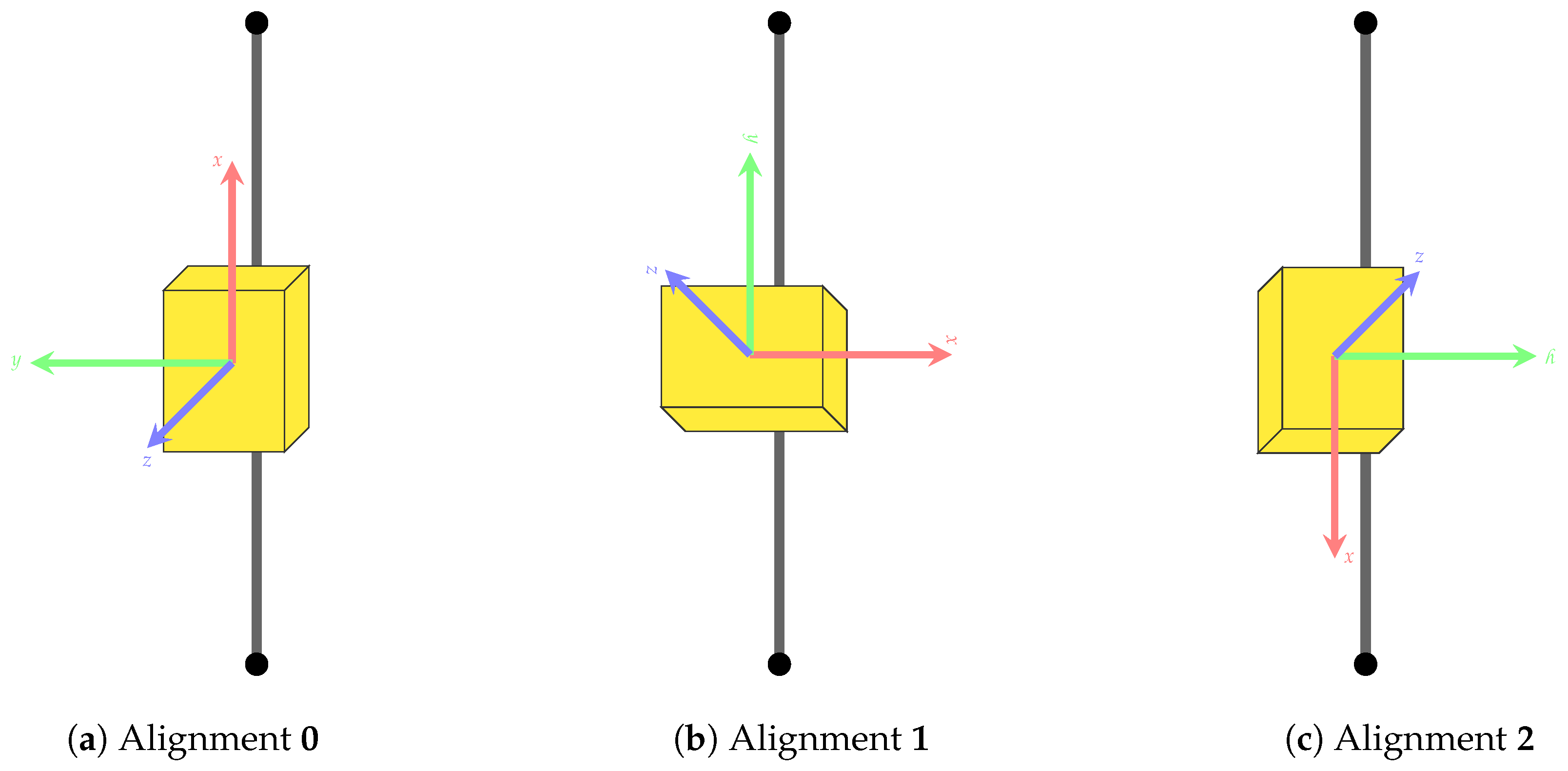
| Placement on Segment | Alignment (See Figure A1) | ||||
|---|---|---|---|---|---|
| # | Upper Leg | Lower Leg | Foot | Pelvis | |
| 1 | anterior | anterior | dorsal | posterior | 0 |
| 2 | anterior | anterior | dorsal | posterior | 1 |
| 3 | anterior | anterior | dorsal | posterior | 2 |
| 4 | lateral | lateral | dorsal | posterior | 0 |
| 5 | lateral | lateral | dorsal | posterior | 1 |
| 6 | lateral | lateral | dorsal | posterior | 2 |
| 7 | anterior | medial | dorsal | posterior | 0 |
| 8 | anterior | medial | dorsal | posterior | 1 |
| 9 | anterior | medial | dorsal | posterior | 2 |
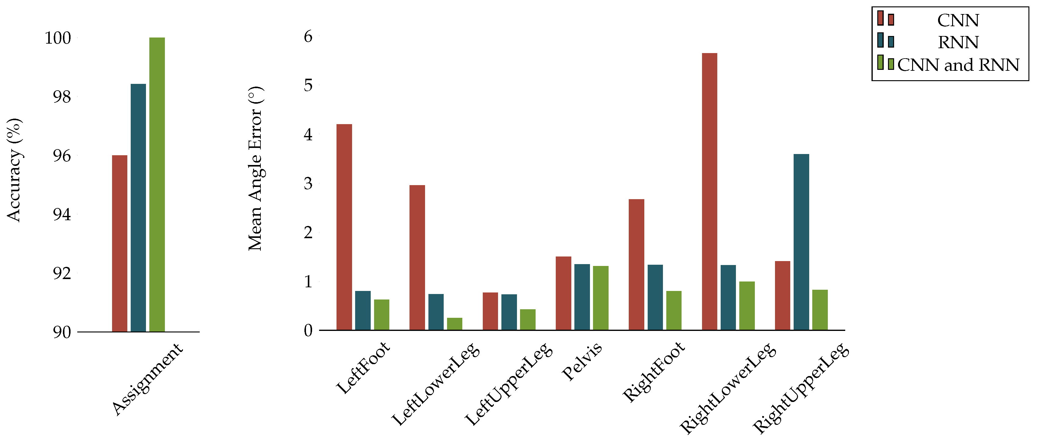
Appendix D. Cross Validation Results on Dataset A
| Accuracy in % | |||
|---|---|---|---|
| CNN | RNN | CNN and RNN | |
| Assignment | 96.00 | 98.43 | 100.00 |
| Mean Angle Errors | |||
|---|---|---|---|
| CNN | RNN | CNN and RNN | |
| LeftFoot | 4.201 | 0.796 | 0.623 |
| LeftLowerLeg | 2.955 | 0.736 | 0.252 |
| LeftUpperLeg | 0.770 | 0.729 | 0.427 |
| Pelvis | 1.503 | 1.347 | 1.309 |
| RightFoot | 2.670 | 1.336 | 0.800 |
| RightLowerLeg | 5.649 | 1.329 | 0.990 |
| RightUpperLeg | 1.407 | 3.589 | 0.822 |
| Mean | 2.736 | 1.405 | 0.795 |
Appendix E. Evaluation Results for the Final Models


| Segment | |||||||||
|---|---|---|---|---|---|---|---|---|---|
| Med | Mean | Max | Med | Mean | Max | Med | Mean | Max | |
| LeftFoot | 1.48 | 13.71 | 165.06 | 2.38 | 6.99 | 44.70 | 4.02 | 12.21 | 155.23 |
| LeftLowerLeg | 4.20 | 28.59 | 178.40 | 3.16 | 14.22 | 75.82 | 7.04 | 17.95 | 116.93 |
| LeftUpperLeg | 1.35 | 14.35 | 171.09 | 0.88 | 8.40 | 81.11 | 1.51 | 10.13 | 96.67 |
| Pelvis | 1.42 | 13.53 | 180.00 | 2.07 | 7.28 | 88.45 | 0.65 | 12.89 | 179.98 |
| RightFoot | 2.96 | 16.12 | 127.48 | 1.35 | 5.23 | 72.81 | 2.39 | 11.42 | 157.63 |
| RightLowerLeg | 3.61 | 31.21 | 179.97 | 7.63 | 10.92 | 52.61 | 5.13 | 24.49 | 179.79 |
| RightUpperLeg | 3.54 | 28.55 | 178.10 | 1.30 | 9.42 | 77.72 | 3.02 | 21.79 | 179.64 |
| Average | 2.65 | 20.86 | 168.58 | 2.68 | 8.92 | 70.46 | 3.39 | 15.84 | 152.26 |
References
- Fong, D.T.P.; Chan, Y.Y. The use of wearable inertial motion sensors in human lower limb biomechanics studies: A systematic review. Sensors 2010, 10, 11556–11565. [Google Scholar] [CrossRef] [PubMed] [Green Version]
- Patel, S.; Park, H.; Bonato, P.; Chan, L.; Rodgers, M. A review of wearable sensors and systems with application in rehabilitation. J. NeuroEng. Rehabil. 2012, 9, 21. [Google Scholar] [CrossRef] [PubMed] [Green Version]
- Hadjidj, A.; Souil, M.; Bouabdallah, A.; Challal, Y.; Owen, H. Wireless sensor networks for rehabilitation applications: Challenges and opportunities. J. Netw. Comput. Appl. 2013, 36, 1–15. [Google Scholar] [CrossRef]
- Zheng, Y.L.; Ding, X.R.; Poon, C.C.Y.; Lo, B.P.L.; Zhang, H.; Zhou, X.L.; Yang, G.Z.; Zhao, N.; Zhang, Y.T. Unobtrusive sensing and wearable devices for health informatics. IEEE Trans. Biomed. Eng. 2014, 61, 1538–1554. [Google Scholar] [CrossRef] [PubMed]
- Bleser, G.; Taetz, B.; Miezal, M.; Christmann, C.A.; Steffen, D.; Regenspurger, K. Development of an Inertial Motion Capture System for Clinical Application—Potentials and challenges from the technology and application perspectives. J. Interact. Media 2017, 16. [Google Scholar] [CrossRef]
- Roetenberg, D.; Luinge, H.; Slycke, P. Xsens MVN: Full 6DOF Human Motion Tracking Using Miniature Inertial Sensors; Technical report; Xsens Technologies: Enschede, The Netherlands, 2014. [Google Scholar]
- Miezal, M.; Taetz, B.; Bleser, G. On Inertial Body Tracking in the Presence of Model Calibration Errors. Sensors 2016, 16, 1132. [Google Scholar] [CrossRef] [PubMed]
- Miezal, M.; Taetz, B.; Bleser, G. Real-time inertial lower body kinematics and ground contact estimation at anatomical foot points for agile human locomotion. In Proceedings of the International Conference on Robotics and Automation, Singapore, 29 May–3 June 2017. [Google Scholar]
- Bouvier, B.; Duprey, S.; Claudon, L.; Dumas, R.; Savescu, A. Upper Limb Kinematics Using Inertial and Magnetic Sensors: Comparison of Sensor-to-Segment Calibrations. Sensors 2015, 15, 18813–18833. [Google Scholar] [CrossRef] [PubMed]
- Palermo, E.; Rossi, S.; Marini, F.; Patané, F.; Cappa, P. Experimental evaluation of accuracy and repeatability of a novel body-to-sensor calibration procedure for inertial sensor-based gait analysis. Measurement 2014, 52, 145–155. [Google Scholar] [CrossRef]
- Taetz, B.; Bleser, G.; Miezal, M. Towards self-calibrating inertial body motion capture. In Proceedings of the International Conference on Information Fusion, Heidelberg, Germany, 5–8 July 2016; pp. 1751–1759. [Google Scholar]
- Weenk, D.; Van Beijnum, B.J.F.; Baten, C.T.; Hermens, H.J.; Veltink, P.H. Automatic identification of inertial sensor placement on human body segments during walking. J. NeuroEng. Rehabil. 2013, 10, 1. [Google Scholar] [CrossRef] [PubMed]
- Graurock, D.; Schauer, T.; Seel, T. Automatic pairing of inertial sensors to lower limb segments—A plug-and-play approach. Curr. Direct. Biomed. Eng. 2016, 2, 715–718. [Google Scholar] [CrossRef]
- De Vries, W.; Veeger, H.; Cutti, A.; Baten, C.; van der Helm, F. Functionally interpretable local coordinate systems for the upper extremity using inertial & magnetic measurement systems. J. Biomech. 2010, 43, 1983–1988. [Google Scholar] [PubMed]
- Favre, J.; Aissaoui, R.; Jolles, B.; de Guise, J.; Aminian, K. Functional calibration procedure for 3D knee joint angle description using inertial sensors. J. Biomech. 2009, 42, 2330–2335. [Google Scholar] [CrossRef] [PubMed]
- Attal, F.; Mohammed, S.; Dedabrishvili, M.; Chamroukhi, F.; Oukhellou, L.; Amirat, Y. Physical Human Activity Recognition Using Wearable Sensors. Sensors 2015, 15, 31314–31338. [Google Scholar] [CrossRef] [PubMed]
- Davis, K.; Owusu, E.; Bastani, V.; Marcenaro, L.; Hu, J.; Regazzoni, C.; Feijs, L. Activity recognition based on inertial sensors for Ambient Assisted Living. In Proceedings of the 19th International Conference on Information Fusion (FUSION), Heidelberg, Germany, 5–8 July 2016; pp. 371–378. [Google Scholar]
- Ordóñez, F.J.; Roggen, D. Deep Convolutional and LSTM Recurrent Neural Networks for Multimodal Wearable Activity Recognition. Sensors 2016, 16, 115. [Google Scholar] [CrossRef] [PubMed]
- Goodfellow, I.; Bengio, Y.; Courville, A. Deep Learning; MIT Press: Cambridge, UK, 2016; Available online: http://www.deeplearningbook.org (accessed on 14 January 2018).
- Ciresan, D.C.; Meier, U.; Masci, J.; Schmidhuber, J. Multi-column deep neural network for traffic sign classification. Neural Netw. 2012, 32, 333–338. [Google Scholar] [CrossRef] [PubMed]
- Krizhevsky, A.; Sutskever, I.; Hinton, G.E. ImageNet Classification with Deep Convolutional Neural Networks. In Advances in Neural Information Processing Systems 25; Pereira, F., Burges, C.J.C., Bottou, L., Weinberger, K.Q., Eds.; Curran Associates, Inc.: New York, NY, USA, 2012; pp. 1097–1105. [Google Scholar]
- Ji, S.; Xu, W.; Yang, M.; Yu, K. 3D Convolutional Neural Networks for Human Action Recognition. IEEE Trans. Pattern Anal. Mach. Intell. 2013, 35, 221–231. [Google Scholar] [CrossRef] [PubMed]
- Tewari, A.; Taetz, B.; Grandidier, F.; Stricker, D. Two Phase Classification for Early Hand Gesture Recognition in 3D Top View Data. In Advances in Visual Computing, Proceedings of the 12th International Symposium, ISVC 2016, Las Vegas, NV, USA, 12–14 December 2016; Springer International Publishing: Basel, Switzerland, 2016; pp. 353–363. [Google Scholar]
- Tewari, A.; Taetz, B.; Frederic, G.; Stricker, D. A Probablistic Combination of CNN and RNN Estimates for Hand Gesture Based Interaction in Car. In Proceedings of the IEEE International Symposium on Mixed and Augmented Reality (ISMAR), Nantes, France, 9–13 October 2017. [Google Scholar]
- Hochreiter, S.; Schmidhuber, J. Long short-term memory. Neural Comput. 1997, 9, 1735–1780. [Google Scholar] [CrossRef] [PubMed]
- Schmidhuber, J. Deep learning in neural networks: An overview. Neural Netw. 2015, 61, 85–117. [Google Scholar] [CrossRef] [PubMed]
- Alsheikh, M.A.; Selim, A.; Niyato, D.; Doyle, L.; Lin, S.; Tan, H.P. Deep Activity Recognition Models with Triaxial Accelerometers. Technical Report. Cornell University Library, 2016. Available online: https://arxiv.org/abs/1511.04664 (accessed on 14 January 2018).
- Morales, F.J.O.N.; Roggen, D. Deep Convolutional Feature Transfer Across Mobile Activity Recognition Domains, Sensor Modalities and Locations. In Proceedings of the 2016 ACM International Symposium on Wearable Computers, Heidelberg, Germany, 12–16 September 2016; ACM: New York, NY, USA, 2016; pp. 92–99. [Google Scholar]
- Kunze, K.; Lukowicz, P. Sensor placement variations in wearable activity recognition. IEEE Pervasive Comput. 2014, 13, 32–41. [Google Scholar] [CrossRef]
- Pannurat, N.; Thiemjarus, S.; Nantajeewarawat, E.; Anantavrasilp, I. Analysis of Optimal Sensor Positions for Activity Classification and Application on a Different Data Collection Scenario. Sensors 2017, 17, 774. [Google Scholar] [CrossRef] [PubMed]
- Kunze, K.; Lukowicz, P. Dealing with Sensor Displacement in Motion-based Onbody Activity Recognition Systems. In Proceedings of the 10th International Conference on Ubiquitous Computing, Seoul, Korea, 21–24 September 2008; ACM: New York, NY, USA, 2008; pp. 20–29. [Google Scholar]
- Jiang, M.; Shang, H.; Wang, Z.; Li, H.; Wang, Y. A method to deal with installation errors of wearable accelerometers for human activity recognition. Physiol. Meas. 2011, 32, 347. [Google Scholar] [CrossRef] [PubMed]
- Henpraserttae, A.; Thiemjarus, S.; Marukatat, S. Accurate Activity Recognition Using a Mobile Phone Regardless of Device Orientation and Location. In Proceedings of the International Conference on Body Sensor Networks, BSN 2011, Dallas, TX, USA, 23–25 May 2011; pp. 41–46. [Google Scholar]
- Kunze, K.; Lukowicz, P.; Junker, H.; Tröster, G. Where am i: Recognizing on-body positions of wearable sensors. In Proceedings of the International Symposium on Location- and Context-Awareness, Oberpfaffenhofen, Germany, 12–13 May 2005; Springer International Publishing: Basel, Switzerland, 2005; pp. 264–275. [Google Scholar]
- Amini, N.; Sarrafzadeh, M.; Vahdatpour, A.; Xu, W. Accelerometer-based on-body sensor localization for health and medical monitoring applications. Pervasive Mob. Comput. 2011, 7, 746–760. [Google Scholar] [CrossRef] [PubMed]
- Mannini, A.; Sabatini, A.M.; Intille, S.S. Accelerometry-based recognition of the placement sites of a wearable sensor. Pervasive Mob. Comput. 2015, 21, 62–74. [Google Scholar] [CrossRef] [PubMed]
- Fujinami, K.; Jin, C.; Kouchi, S. Tracking on-body location of a mobile phone. In Proceedings of the International Symposium on Wearable Computers, Seoul, Korea, 10–13 October 2010; pp. 190–197. [Google Scholar]
- Kunze, K.; Lukowicz, P. Using acceleration signatures from everyday activities for on-body device location. In Proceedings of the 2007 11th IEEE International Symposium on Wearable Computers, Boston, MA, USA, 11–13 October 2007; 2007; pp. 115–116. [Google Scholar]
- Xu, W.; Zhang, M.; Sawchuk, A.A.; Sarrafzadeh, M. Robust human activity and sensor location corecognition via sparse signal representation. IEEE Trans. Biomed. Eng. 2012, 59, 3169–3176. [Google Scholar] [PubMed]
- Shi, Y.; Shi, Y.; Liu, J. A Rotation Based Method for Detecting On-body Positions of Mobile Devices. Proceedings of the 13th International Conference on Ubiquitous Computing, Beijing, China, 17–21 September 2011; ACM: New York, NY, USA, 2011; pp. 559–560.
- Thiemjarus, S. A Device-Orientation Independent Method for Activity Recognition. In Proceedings of the International Conference on Body Sensor Networks, BSN 2010, Singapore, 7–9 June 2010; pp. 19–23. [Google Scholar]
- Young, A.D.; Ling, M.J.; Arvind, D.K. IMUSim: A Simulation Environment for Inertial Sensing Algorithm Design and Evaluation. In Proceedings of the 10th International Conference on Information Processing in Sensor Networks, Chicago, IL, USA, 12–14 April 2011; pp. 199–210. [Google Scholar]
- Brunner, T.; Lauffenburger, J.; Changey, S.; Basset, M. Magnetometer-Augmented IMU Simulator: In-Depth Elaboration. Sensors 2015, 15, 5293–5310. [Google Scholar] [CrossRef] [PubMed]
- Ligorio, G.; Bergamini, E.; Pasciuto, I.; Vannozzi, G.; Cappozzo, A.; Sabatini, A.M. Assessing the Performance of Sensor Fusion Methods: Application to Magnetic-Inertial-Based Human Body Tracking. Sensors 2016, 16, 153. [Google Scholar] [CrossRef] [PubMed]
- Zhang, X.; Fu, Y.; Jiang, S.; Sigal, L.; Agam, G. Learning from Synthetic Data Using a Stacked Multichannel Autoencoder. Technical Report. Cornell University Library, 2015. Available online: https://arxiv.org/abs/1509.05463 (accessed on 14 January 2018).
- Le, T.A.; Baydin, A.G.; Zinkov, R.; Wood, F. Using Synthetic Data to Train Neural Networks is Model-Based Reasoning. arXiv, 2017; arXiv:1703.00868v1. [Google Scholar]
- Zhang, X.; Fu, Y.; Zang, A.; Sigal, L.; Agam, G. Learning Classifiers from Synthetic Data Using a Multichannel Autoencoder. Technical Report. Cornell University Library, 2015. Available online: https://arxiv.org/abs/1503.03163 (accessed on 14 January 2018).
- Simard, P.Y.; Steinkraus, D.; Platt, J.C. Best Practices for Convolutional Neural Networks Applied to Visual Document Analysis. In Proceedings of the Seventh International Conference on Document Analysis and Recognition (ICDAR ’03), Edinburgh, UK, 3–6 August 2003; IEEE Computer Society: Washington, DC, USA, 2003. [Google Scholar]
- University, C.M. CMU Graphics Lab Motion Capture Database Website. Available online: http://mocap.cs.cmu.edu/ (accessed on 14 January 2018).
- Ioffe, S.; Szegedy, C. Batch normalization: Accelerating deep network training by reducing internal covariate shift. In Proceedings of the International Conference on Machine Learning, Lille, France, 6–1 July 2015; pp. 448–456. [Google Scholar]
- Bengio, Y.; Simard, P.; Frasconi, P. Learning long-term dependencies with gradient descent is difficult. IEEE Trans. Neural Netw. 1994, 5, 157–166. [Google Scholar] [CrossRef] [PubMed]
- Cho, K.; van Merrienboer, B.; Gülcehre, C.; Bahdanau, D.; Bougares, F.; Schwenk, H.; Bengio, Y. Learning Phrase Representations using RNN Encoder-Decoder for Statistical Machine Translation; EMNLP; Moschitti, A., Pang, B., Daelemans, W., Eds.; Association for Computational Linguistics: Doha, Qatar, 2014; pp. 1724–1734. [Google Scholar]
- Gal, Y. Uncertainty in Deep Learning. Ph.D. Thesis, University of Cambridge, Cambridge, UK, 2016. [Google Scholar]
- Srivastava, N.; Hinton, G.E.; Krizhevsky, A.; Sutskever, I.; Salakhutdinov, R. Dropout: A simple way to prevent neural networks from overfitting. J. Mach. Learn. Res. 2014, 15, 1929–1958. [Google Scholar]
- Gal, Y. A Theoretically Grounded Application of Dropout in Recurrent Neural Networks. arXiv, 2015; arXiv:1512.05287. [Google Scholar]
- Terzakis, G.; Culverhouse, P.; Bugmann, G.; Sharma, S.; Sutton, R. A Recipe on the Parameterization of Rotation Matrices for Non-Linear Optimization Using Quaternions; Technical report, Technical report MIDAS. SMSE. 2012. TR. 004; Marine and Industrial Dynamic Analysis School of Marine Science and Engineering, Plymouth University: Plymouth, UK, 2012. [Google Scholar]
- Xsens Technologies B.V. Available online: https://www.xsens.com/products/xsens-mvn/ (accessed on 14 January 2018).
- Shuster, M.D. A survey of attitude representations. Navigation 1993, 8, 439–517. [Google Scholar]
- Butterworth, S. On the theory of filter amplifiers. Wirel. Eng. 1930, 7, 536–541. [Google Scholar]
- NaturalPoint OptiTrack. Available online: http://www.optitrack.com/motion-capture-biomechanics/ (accessed on 14 January 2018).
- Olsson, F.; Halvorsen, K. Experimental evaluation of joint position estimation using inertial sensors. In Proceedings of the 20th International Conference on Information Fusion (Fusion), IEEE, Xi’an, China, 10–13 July 2017; pp. 1–8. [Google Scholar]
- Mohammed, S.; Tashev, I. Unsupervised deep representation learning to remove motion artifacts in free-mode body sensor networks. In Proceedings of the 14th IEEE International Conference on Wearable and Implantable Body Sensor Networks (BSN), Eindhoven, The Netherlands, 9–12 May 2017; pp. 183–188. [Google Scholar]
- Abadi, M.; Agarwal, A.; Barham, P.; Brevdo, E.; Chen, Z.; Citro, C.; Corrado, G.S.; Davis, A.; Dean, J.; Devin, M.; et al. Tensorflow: Large-scale machine learning on heterogeneous distributed systems. arXiv, 2016; arXiv:1603.04467. [Google Scholar]
- Golyanik, V.; Reis, G.; Taetz, B.; Strieker, D. A framework for an accurate point cloud based registration of full 3D human body scans. In Proceedings of the 2017 Fifteenth IAPR International Conference on Machine Vision Applications (MVA), Nagoya, Japan, 8–12 May 2017; pp. 67–72. [Google Scholar]
- Bahdanau, D.; Cho, K.; Bengio, Y. Neural machine translation by jointly learning to align and translate. arXiv, 2014; arXiv:1409.0473. [Google Scholar]


© 2018 by the authors. Licensee MDPI, Basel, Switzerland. This article is an open access article distributed under the terms and conditions of the Creative Commons Attribution (CC BY) license (http://creativecommons.org/licenses/by/4.0/).
Share and Cite
Zimmermann, T.; Taetz, B.; Bleser, G. IMU-to-Segment Assignment and Orientation Alignment for the Lower Body Using Deep Learning. Sensors 2018, 18, 302. https://doi.org/10.3390/s18010302
Zimmermann T, Taetz B, Bleser G. IMU-to-Segment Assignment and Orientation Alignment for the Lower Body Using Deep Learning. Sensors. 2018; 18(1):302. https://doi.org/10.3390/s18010302
Chicago/Turabian StyleZimmermann, Tobias, Bertram Taetz, and Gabriele Bleser. 2018. "IMU-to-Segment Assignment and Orientation Alignment for the Lower Body Using Deep Learning" Sensors 18, no. 1: 302. https://doi.org/10.3390/s18010302
APA StyleZimmermann, T., Taetz, B., & Bleser, G. (2018). IMU-to-Segment Assignment and Orientation Alignment for the Lower Body Using Deep Learning. Sensors, 18(1), 302. https://doi.org/10.3390/s18010302