An Improved Coarse Alignment Algorithm for Odometer-Aided SINS Based on the Optimization Design Method


College of Automation, Harbin Engineering University, Harbin 150001, China
*
Author to whom correspondence should be addressed.
Sensors 2018, 18(1), 195; https://doi.org/10.3390/s18010195
Submission received: 2 November 2017
/
Revised: 24 December 2017
/
Accepted: 10 January 2018
/
Published: 11 January 2018
(This article belongs to the Special Issue Inertial Sensors for Positioning and Navigation)
Abstract
:An improved coarse alignment (ICA) algorithm is proposed in this paper with a focus on improving alignment accuracy of odometer-aided strapdown inertial navigation system (SINS) under variable velocity and variable acceleration condition. In the proposed algorithm, the outputs of inertial sensors and odometer in a sampling interval are linearized rather than assumed to be a constant, which improves the accuracy of the vector observations and the precision of coarse alignment. Simulation and field test results illustrate that, under variable velocity and variable acceleration condition, the proposed algorithm can obtain a better alignment performance than conventional coarse alignment method.
1. Introduction
[-15]Strapdown inertial navigation system (SINS) can autonomously, continuously and comprehensively provide the position, velocity, and attitude of the carrier [1,2,3,4]. The performance of SINS depends on the accuracy and rapidity of the initial alignment process, which can be divided into coarse alignment and fine alignment [5,6]. Coarse alignment is important since it provides a rapidly alignment result for the fine alignment. The existing algorithms of the coarse alignment mainly include: analytic coarse alignment [7,8,9], inertial frame coarse alignment (IFCA) [10,11], and coarse alignment based on Davenport’s q method [12,13,14,15,16]. The analytic coarse alignment can only be used on static base. In order to solve moving base coarse alignment problem, some IFCA algorithms have been proposed. In [13], Li et al. proposes a fast SINS initial alignment method based on IFCA with the aid of external reference velocity. However, this algorithm has the problem of large random errors. In [15,17,18], the optimization-based alignment (OBA) method with the aid of external reference information provided by Global Navigation Satellite System (GNSS) is proposed. The OBA algorithm obtains optimal attitude matrix through the q method to reduce random errors of attitude angles, however, these algorithms in [15,17] are not suitable for odometer-aided SINS, since the odometer can only provide the velocity in body frame. To solve this problem, the OBA algorithm with the aid of external velocity provided by odometer is reported in [19,20,21]. However, the outputs of inertial sensors and odometer in one sampling interval are assumed to be a constant, which may result in errors of coarse alignment when the velocity and acceleration change.
In order to improve the alignment performance under changeable velocity and acceleration, an improved coarse alignment (ICA) algorithm for SINS aided by odometer is proposed in this paper. The main contribution is that the outputs of inertial sensors and odometer that are assumed to be a constant in a sampling interval in [15,17,19] are replaced by their linear approximations to improve the accuracy of the integral formulae of vector observations. Experimental results show that the proposed ICA algorithm has better accuracy than the OBA algorithm and the traditional IFCA algorithm especially when the velocity and acceleration change, which is more suitable for coarse alignment of odometer-aided SINS.
This paper is organized as follows. Section 2 introduces the OBA algorithm for odometer-aided SINS. Section 3 derives the proposed ICA algorithm with linear approximation of inertial sensors and odometer. Simulation results and field test results are reported in Section 4. Finally, conclusions are drawn in Section 5.
2. OBA Algorithm for Odometer-Aided SINS
The coarse alignment aims at determining a coordinate transformation matrix in a short time, where n denotes the local level navigation frame and b denotes the body frame, respectively. In this paper, we denote by i the inertial frame and e the earth frame. The kinematic equations of navigation are known as [1,15,19]
where denotes the ground velocity in the navigation frame, is the earth rotation angular velocity, denotes the angular rate of the navigation fame with respect to the earth frame, and is the specific force measured by accelerometers. is the body angular rate measured by gyroscope, and represents the angular rate of the body frame with respect to the navigation frame. Moreover, denotes the local gravity acceleration, and denotes the cross product matrix. According to the chain rule, the attitude transformation matrix can be decomposed as
where and denote the change of body frame and navigation frame from time 0 to , respectively. They are calculated by the following differential equations
where denotes the angular rate of the navigation frame with respect to the inertial frame.
After obtaining the attitude matrixes and by Equations (4) and (5), the key problem to determine is to obtain the constant matrix . The specific force Equation (2) is used as the measurement equation in the OBA algorithm with the aid of velocity in navigation frame, such as GNSS, and it can be rewritten as follows if the velocity is provided in body frame, such as the odometer
Substituting (3) into (6) and integrating the specific force equation from time interval 0 to t, we have
The next step is to calculate the vector observations and . In [15,17,19], the output of accelerometer , the output of gyroscope and the output of odometer are all assumed to be constants in a sampling interval, which may result in errors in when velocity and acceleration are changing. Next we will propose an ICA algorithm by linearizing these outputs in sampling intervals.
3. ICA Algorithm for Odometer-Aided SINS
In the following, T represents the time period of the update interval , , and the current time is , where M is the sampling number. Ignoring the change of gravity acceleration , the vector observation is written as
Since the angular rate of navigation frame with respect to inertial frame changes slowly, can be approximated as [15]
where denotes the navigation frame rotation vector from to , and is approximated as
The first integral term in Equation (9) can be written as
In order to improve the accuracy of the vector observations, we make a linear approximation for the outputs and of SINS. Suppose that changes linearly during the period of and can be approximated as
Similarly, can be approximated as a linear form
where
The output of the odometer contained in the second integral in (9) can also be approximated as
The term is calculated as follows
Substituting Equations (19), (23) and (26) into Equation (9), the second integral term in (9) can be approximated as
The vector observation is abbreviated as
Then the discrete measurement equation can be rewritten in a compact form
After obtaining the vector observations, the measurement Equation (29) can be solved by the method. The constant matrix can be formulated by its corresponding quaternion , subject to
where s is scalar part and is the vector part. The vector observations can be written in the form of quaternion
It is convenient to make Equation (29) equivalent to , where ∘ denotes the quaternion multiplication and is the conjugate quaternion of . The quaternion multiplication matrix is defined as
Thus, the attitude quaternion can be determined by solving the following optimization problem
where
It can be proved that J in Equation (35) will be minimized if is chosen to be the eigenvector corresponding to the smallest eigenvalue of , which is the optimal quaternion related to [15,18]. The block diagram of the ICA algorithm is shown in Figure 1. In Figure 1, LA denotes the process of linear approximation for the outputs of inertial sensors and odometer, AUb and AUn denote update processes of attitude matrix and attitude matrix , respectively, and the q method is used to calculate the attitude matrix . According to the chain rule, the attitude matrix can be updated in real time by Equation (3). In conclusion, the attitude matrix can be calculated through the ICA algorithm in real time by Equations (3)–(5) and (29).
4. Simulation and Test
4.1. Simulation Results
We first give simulation results under variable velocity and acceleration condition for coarse alignment of odometer-aided SINS using the proposed ICA algorithm. In order to verify the performance of the ICA algorithm, the in-motion model with severe maneuvering was built. The swing motion are set as sine functions
where , and are the amplitudes and set as , , and , respectively. , and are swing periods, which are set as , and , respectively. , and are initial phases and they are random values in the range from 0 radian to radian, , and are initial attitude angles and they are random values in the range from to . The initial parameters of the simulation are shown in Table 1. As is shown in Table 1, the random error of the gyroscope and accelerometer are set as Gaussian white noise, and the standard deviation of the gyroscope noise and accelerometer noise are and , respectively.
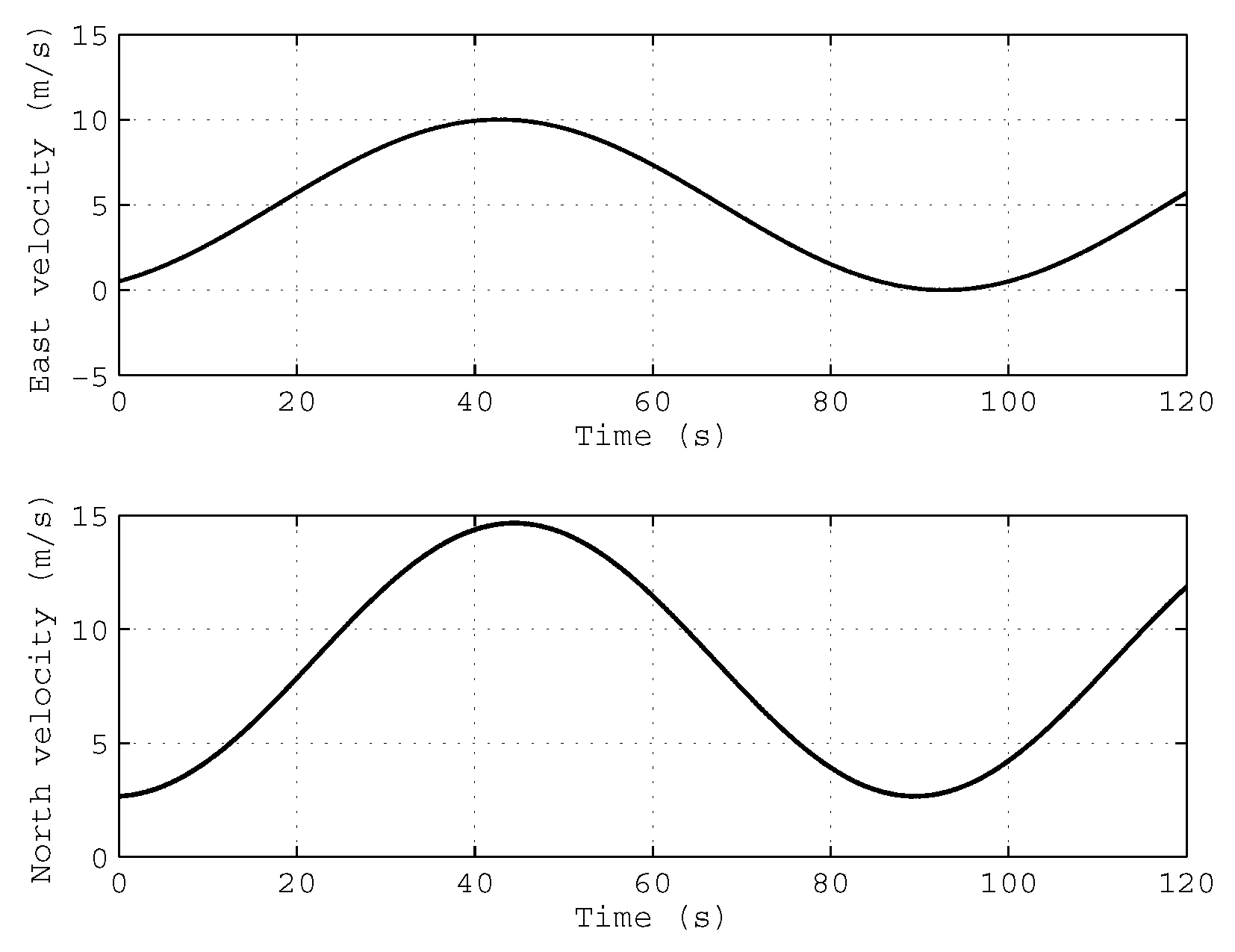
In order to simulate the condition of variable velocity and variable acceleration, the velocity of the vehicle is set as a sine-cosine function in the navigation frame, and the velocity of the vehicle is shown in Figure 2.
The first simulation lasts about 150 s under the condition of variable velocity and variable acceleration, and the simulation results of the OBA algorithm and the proposed ICA algorithm are shown in Figure 3. Figure 3 shows that the errors of the roll angle and pitch angle are all less than after 10 s, and the heading error obtained by the proposed ICA algorithm is less than after 80 s. Compared with the OBA algorithm, the heading angle calculated by the ICA algorithm can obtain more accurate results with faster convergence speed.
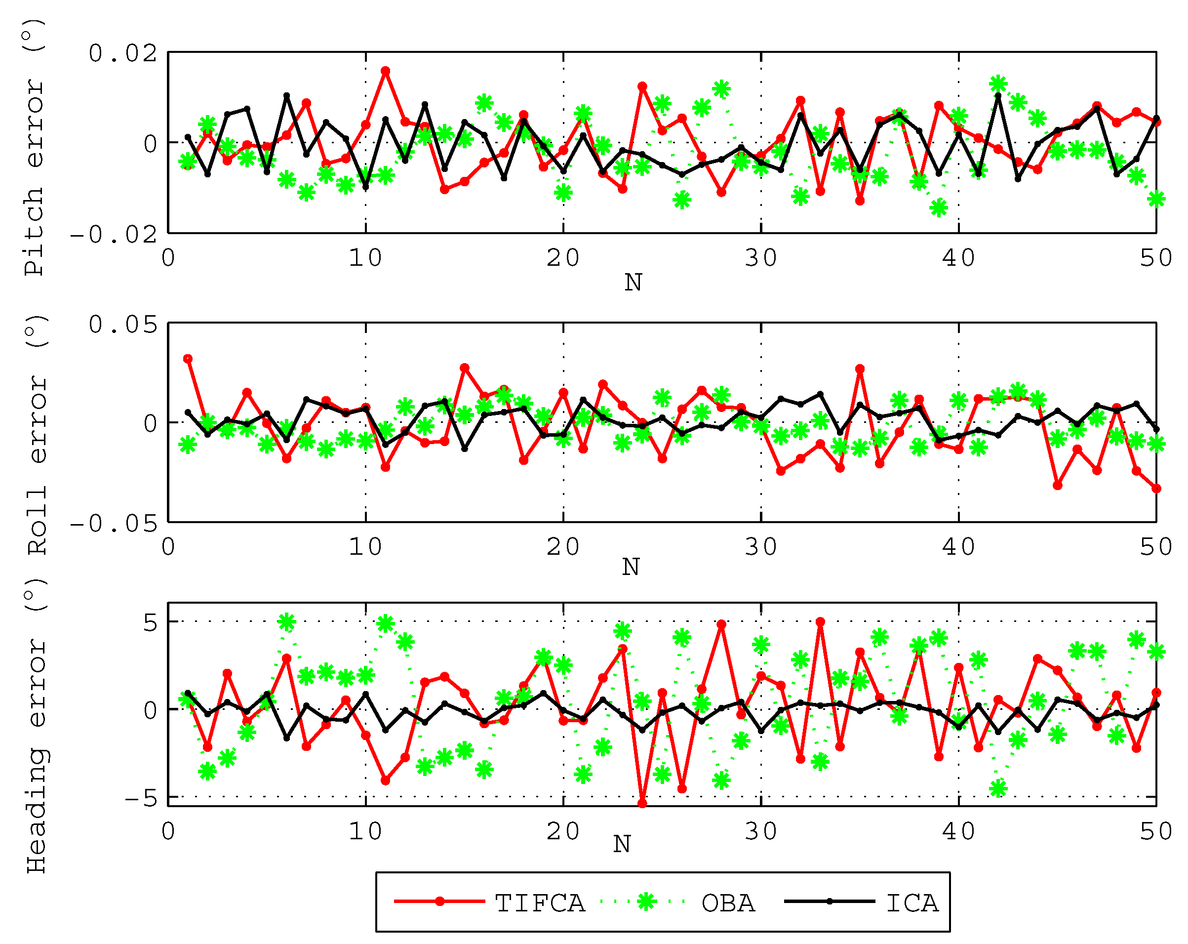
To further show the advantage of the proposed algorithm, 50 coarse alignment trials are performed. Each coarse alignment lasts 100 s, and the final attitude angles are chosen as the alignment results. Figure 4 gives the results of the three kinds of typical coarse alignment algorithms. The black line denotes the results of the proposed ICA algorithm, the green line denotes the results of the OBA algorithm aided by odometer [19], and the red line denotes the results of the traditional IFCA method (TIFCA) aided by odometer [13]. The statistics of the attitude angle errors through three algorithms are shown in Table 2.
Figure 4 and Table 2 show that the errors of the level attitude angle, pitch angle and roll angle, are all less than . However, the TIFCA algorithm and the OBA algorithm have a poor performance on heading alignment, and we can see from Table 2 that the heading error of the two algorithms are more than and standard deviation is greater than . The heading error of the proposed ICA algorithm is less than at 100 s, and the standard deviation reduces to . The standard deviation of the heading angel error adopting ICA algorithm is obviously smaller than the other two algorithms. Both pitch and roll angles can be accurate and quickly obtained by all algorithms, and there is no big difference in the results. The difficulty of coarse alignment is the estimation of the heading angle, especially on variable velocity and variable acceleration condition. As is shown in simulation results, compared with the TIFCA algorithm and OBA algorithm, the proposed algorithm has a better alignment performance under the condition of variable velocity and variable acceleration.
4.2. Test Results
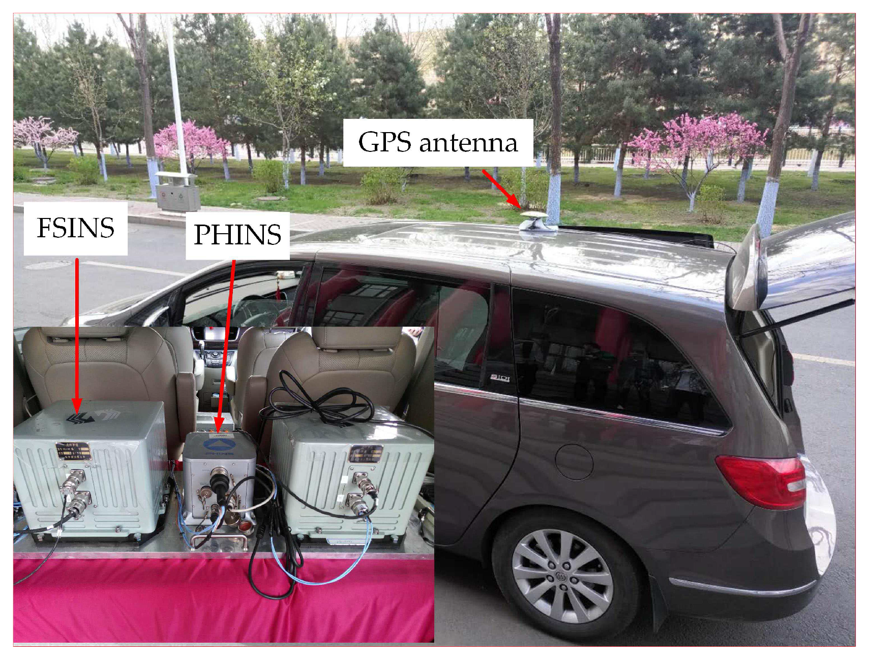
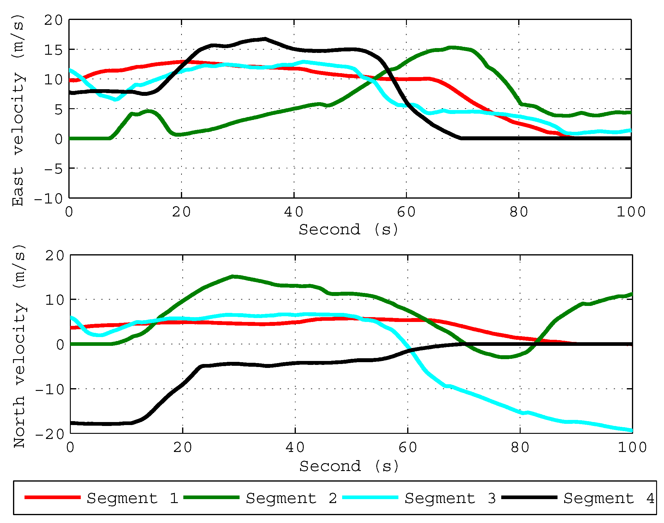
In order to verify the validity of the proposed ICA algorithm in practice, we carried out a field test to verify the performance of the ICA algorithm. As is shown in Figure 5, the self-made fiber-optic-SINS (FSINS) and photonics inertial navigation system (PHINS) are installed together on a reference platform inside the car, and the GPS antenna is installed outside on the top of the car. The position of the experiment is and . The initial position for each coarse alignment is provided by GPS, and the ground velocity in the body frame is provided by the odometer. The specific force and the body angler rate are provided by FSINS, and the FSINS is equipped with gyroscopes (drift , noise ) and accelerometers (bias , noise ). The attitude angles provided by the GPS/PHINS integrated navigation system are used as the attitude reference, and the specifications of GPS/PHINS integrated navigation system are listed in Table 3. The car was moving severely with the change of velocity and acceleration. We carried out four coarse alignments, and each alignment data segment lasts 100 s with the feature of variable velocity and variable acceleration. Figure 6 shows the velocity changes of four segments.
The coarse alignment results of three algorithms are listed in Table 4, Table 5 and Table 6, in which final attitude angle errors of four coarse alignments are defined as the differences between final attitude angles of three algorithms and the outputs of the reference. As is shown in Table 4 and Table 5, the level attitude errors of three algorithms all reduce to values less than in , which fulfill the accuracy requirement of coarse alignment. Table 6 shows the final heading angle errors of four segments. As is shown in Table 6, the heading angle errors of the four segments obtained by the proposed ICA algorithm are all smaller than the other two algorithms. In conclusion, under the variable velocity and variable acceleration condition, the ICA algorithm has a better performance in coarse alignment of odometer-aided SINS, and the test results coincide with the simulation results.
5. Conclusions
To overcome the performance degradation of the existing TIFCA and OBA algorithms under variable velocity and variable acceleration conditions, a novel improved coarse alignment algorithm for odometer-aided SINS is proposed in this paper. By constructing the vector observations with a linear approximation of sensors’ outputs, the proposed algorithm is able to obtain better accuracy than existing TIFCA and OBA algorithms. Simulation results and field tests verified the performance that the proposed algorithm can obtain smaller heading angle errors, which is more suitable for odometer-aided SINS coarse alignment.
Acknowledgments
This work was supported by the National Natural Science Foundation of China under Grant Nos. 61773133 and 61633008 and the Natural Science Foundation of Heilongjiang Province Grant No. F2016008. The authors would like to thank all the editors and anonymous reviewers for improving this article.
Author Contributions
Yonggang Zhang and Li Luo conceived and designed the experiments; Li Luo performed the experiment; Yonggang Zhang contributed experiment tools and analyzed the data; Li Luo, Tao Fang, Ning Li and Guoqing Wang wrote the paper.
Conflicts of Interest
The authors declare no conflict of interest.
References
- Tang, Y.; Wu, Y.; Wu, M.; Wu, W.; Hu, X.; Shen, L. INS/GPS Integration: Global Observability Analysis. IEEE. Trans. Veh. Technol. 2009, 58, 1129–1142. [Google Scholar] [CrossRef]
- Huang, W.; Fang, T.; Luo, L.; Zhao, L.; Che, F. A Damping Grid Strapdown Inertial Navigation System Based on a Kalman Filter for Ships in Polar Regions. Sensors 2017, 17, 1551. [Google Scholar]
- Zhang, Y.; Huang, Y.; Wu, Z.; Li, N. Moving State Marine SINS Initial Alignment Based on High Degree CKF. Math. Probl. Eng. 2014, 2014, 546107. [Google Scholar] [CrossRef]
- Huang, Y.; Zhang, Y. A New Process Uncertainty Robust Student’s t based Kalman Filter for SINS/GPS Integration. IEEE Access 2017, 5, 14391–14404. [Google Scholar] [CrossRef]
- Lu, J.; Lei, C.; Li, B.; Wen, T. Improved calibration of IMU biases in analytic coarse alignment for AHRS. Meas. Sci. Technol. 2016, 27, 075105. [Google Scholar] [CrossRef]
- Huang, Y.; Zhang, Y.; Wang, X. Kalman-Filtering-Based In-Motion Coarse Alignment for Odometer-Aided SINS. IEEE Trans. Instrum. Meas. 2017, PP, 1–14. [Google Scholar] [CrossRef]
- Shuster, M.D.; Oh, S.D. Three-axis attitude determination from vector observations. J. Guid. Control Dyn. 1981, 4, 70–77. [Google Scholar] [CrossRef]
- Jiang, Y.F. Error analysis of analytic coarse alignment methods. IEEE. Trans. Aerosp. Electron. Syst. 1998, 34, 334–337. [Google Scholar] [CrossRef]
- Tan, C.; Zhu, X.; Su, Y.; Wang, Y.; Wu, Z.; Gu, D. A New Analytic Alignment Method for a SINS. Sensors 2015, 15, 27930–27953. [Google Scholar] [CrossRef] [PubMed]
- Li, J.; Fang, J.; Du, M. Error Analysis and Gyro-Bias Calibration of Analytic Coarse Alignment for Airborne POS. IEEE Trans. Instrum. Meas. 2012, 61, 3058–3064. [Google Scholar]
- Zhou, W.D.; Ma, H.; Ji, Y.R.; Song, J.L. Coarse Alignment for SINS Using Gravity in the Inertial Frame Based on Attitude Quaternion. Appl. Mech. Mater. 2013, 244, 413–417. [Google Scholar] [CrossRef]
- Zhang, T.; Zhu, Y.; Zhou, F.; Yan, Y.; Tong, J. Coarse Alignment Technology on Moving Base for SINS Based on the Improved Quaternion Filter Algorithm. Sensors 2017, 17, 1424. [Google Scholar] [CrossRef] [PubMed]
- Li, W.; Wu, W.; Lu, J.W.L. A Fast SINS Initial Alignment Scheme for Underwater Vehicle Applications. J. Navig. 2013, 66, 181–198. [Google Scholar] [CrossRef]
- Wu, M.; Wu, Y.; Hu, X.; Hu, D. Optimization-based alignment for inertial navigation systems: Theory and algorithm. Aerosp. Sci. Technol. 2011, 15, 1–17. [Google Scholar] [CrossRef]
- Wu, Y.; Pan, X. Velocity/Position Integration Formula Part I: Application to In-Flight Coarse Alignment. IEEE Trans. Aerosp. Electron. Syst. 2013, 49, 1006–1023. [Google Scholar] [CrossRef]
- Chang, L.; Li, J.; Chen, S. Initial Alignment by Attitude Estimation for Strapdown Inertial Navigation Systems. IEEE Trans. Instrum. Meas. 2015, 64, 784–794. [Google Scholar] [CrossRef]
- Chang, L.; Li, J.; Li, K. Optimization-based alignment for strapdown inertial navigation system: Comparison and extension. IEEE Trans. Aerosp. Electron. Syst. 2016, 52, 1697–1713. [Google Scholar] [CrossRef]
- Chang, L.; Qin, F.; Li, A. A Novel Backtracking Scheme for Attitude Determination-Based Initial Alignment. IEEE Trans. Autom. Sci. Eng. 2015, 12, 384–390. [Google Scholar] [CrossRef]
- Kang, L.; Ye, L.; Song, K. A fast in-motion alignment algorithm for DVL aided SINS. Math. Probl. Eng. 2014, 2014, 593692. [Google Scholar] [CrossRef]
- Chang, L.; He, H.; Qin, F. In-motion Initial Alignment for Odometer Aided Strapdown Inertial Navigation System based on Attitude Estimation. IEEE Sens. J. 2017, 17, 766–773. [Google Scholar] [CrossRef]
- Chang, L.; Li, Y.; Xue, B. Initial Alignment for Doppler Velocity Log aided Strapdown Inertial Navigation System with Limited Information. IEEE ASME Trans. Mechatron. 2017, 22, 329–338. [Google Scholar] [CrossRef]
Figure 1.
The block diagram of the proposed ICA algorithm.
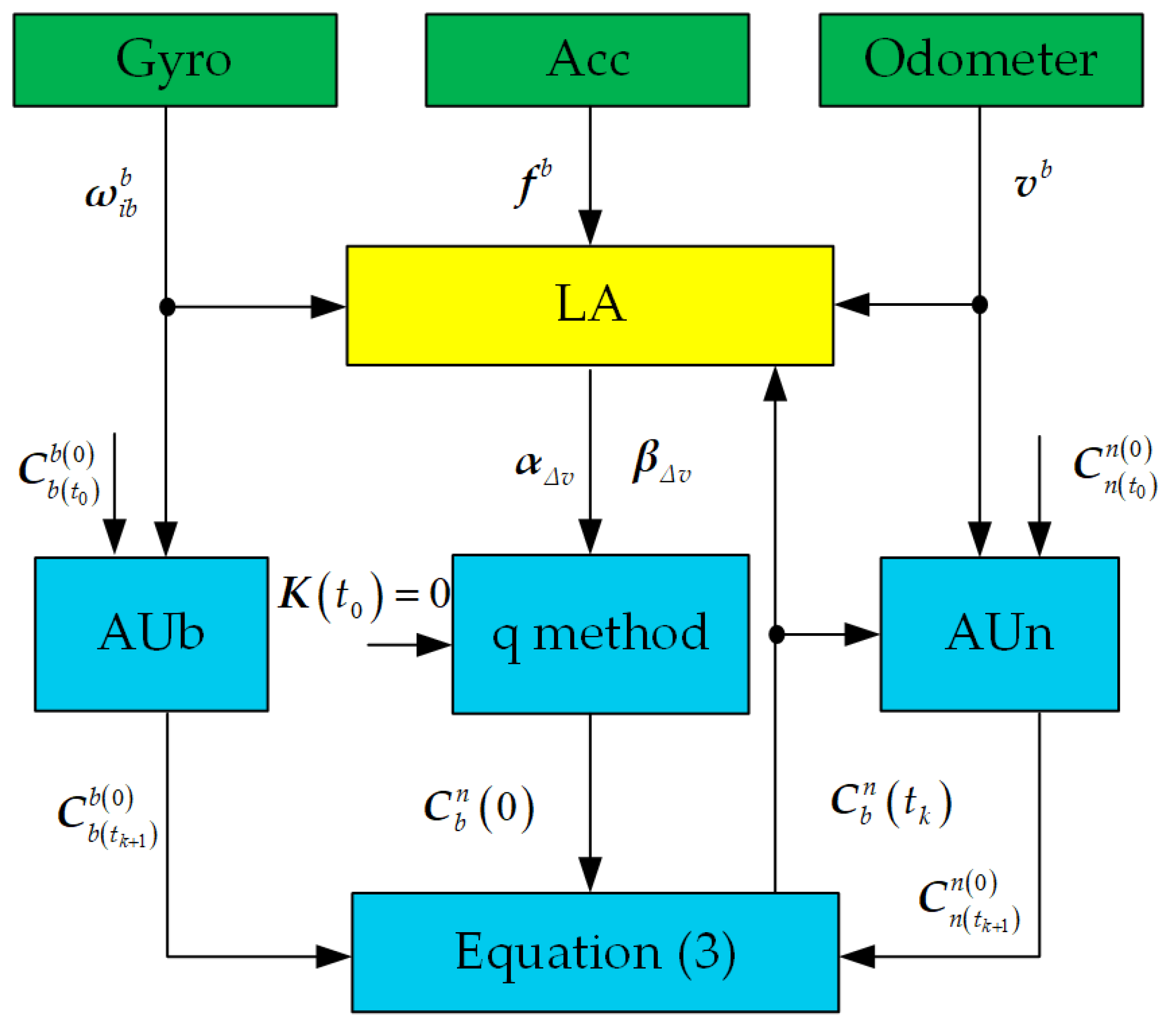
Figure 2.
The true velocity profile of the simulation test.

Figure 3.
The attitude angle error of the simulation.
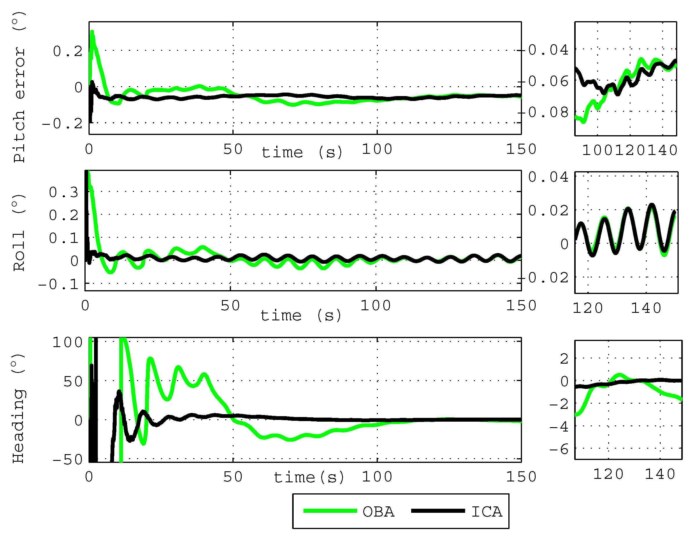
Figure 4.
The attitude angle errors of 50 coarse alignments. The abscissa denotes the order of the alignments, and the ordinate denotes the errors of the pitch angle, roll angle and heading angle, respectively.
Figure 4.
The attitude angle errors of 50 coarse alignments. The abscissa denotes the order of the alignments, and the ordinate denotes the errors of the pitch angle, roll angle and heading angle, respectively.

Figure 5.
The FSINS and PHINS for the experiment.

Figure 6.
Velocity profile for four segments.


Table 1.
Initial parameters.
| Parameter Name | Parameter Value |
|---|---|
| Initial longitude | |
| Initial latitude L | |
| Fiber-optic gyroscope drift | |
| Fiber-optic gyroscope noise | |
| Accelerometer bias | |
| Accelerometer noise | |
| odometer noise |
Table 2.
The simulation result of 50 coarse alignments.
| Attitude Angle | Method | Maximum Error | Mean Error | Standard Deviation |
|---|---|---|---|---|
| Pitch | TIFCA | |||
| OBA | ||||
| ICA | ||||
| Roll | TIFCA | |||
| OBA | ||||
| ICA | ||||
| Heading | TIFCA | |||
| OBA | ||||
| ICA |
Table 3.
Specifications of the GPS/PHINS integrated navigation system.
| Index | Accuracy |
|---|---|
| Heading, Roll, Pitch resolution | |
| Heading, Roll, Pitch dynamic accuracy | |
| Saturation of the speed | |
| Speed accuracy | |
| The position error of GPS receiver | ≤10 m |
Table 4.
The final pitch angle error of four segments.
| Data | TIFCA | OBA | ICA |
|---|---|---|---|
| Segment 1 | |||
| Segment 2 | |||
| Segment 3 | |||
| Segment 4 |
Table 5.
The final roll angle error of four segments.
| Data | TIFCA | OBA | ICA |
|---|---|---|---|
| Segment 1 | |||
| Segment 2 | |||
| Segment 3 | |||
| Segment 4 |
Table 6.
The final heading angle error of four segments.
| Data | TIFCA | OBA | ICA |
|---|---|---|---|
| Segment 1 | |||
| Segment 2 | |||
| Segment 3 | |||
| Segment 4 |
© 2018 by the authors. Licensee MDPI, Basel, Switzerland. This article is an open access article distributed under the terms and conditions of the Creative Commons Attribution (CC BY) license (http://creativecommons.org/licenses/by/4.0/).
Share and Cite
MDPI and ACS Style
Zhang, Y.; Luo, L.; Fang, T.; Li, N.; Wang, G. An Improved Coarse Alignment Algorithm for Odometer-Aided SINS Based on the Optimization Design Method. Sensors 2018, 18, 195. https://doi.org/10.3390/s18010195
AMA Style
Zhang Y, Luo L, Fang T, Li N, Wang G. An Improved Coarse Alignment Algorithm for Odometer-Aided SINS Based on the Optimization Design Method. Sensors. 2018; 18(1):195. https://doi.org/10.3390/s18010195
Chicago/Turabian StyleZhang, Yonggang, Li Luo, Tao Fang, Ning Li, and Guoqing Wang. 2018. "An Improved Coarse Alignment Algorithm for Odometer-Aided SINS Based on the Optimization Design Method" Sensors 18, no. 1: 195. https://doi.org/10.3390/s18010195
Note that from the first issue of 2016, this journal uses article numbers instead of page numbers. See further details here.