
A Framework Based on Reference Data with Superordinate Accuracy for the Quality Analysis of Terrestrial Laser Scanning-Based Multi-Sensor-Systems


Abstract
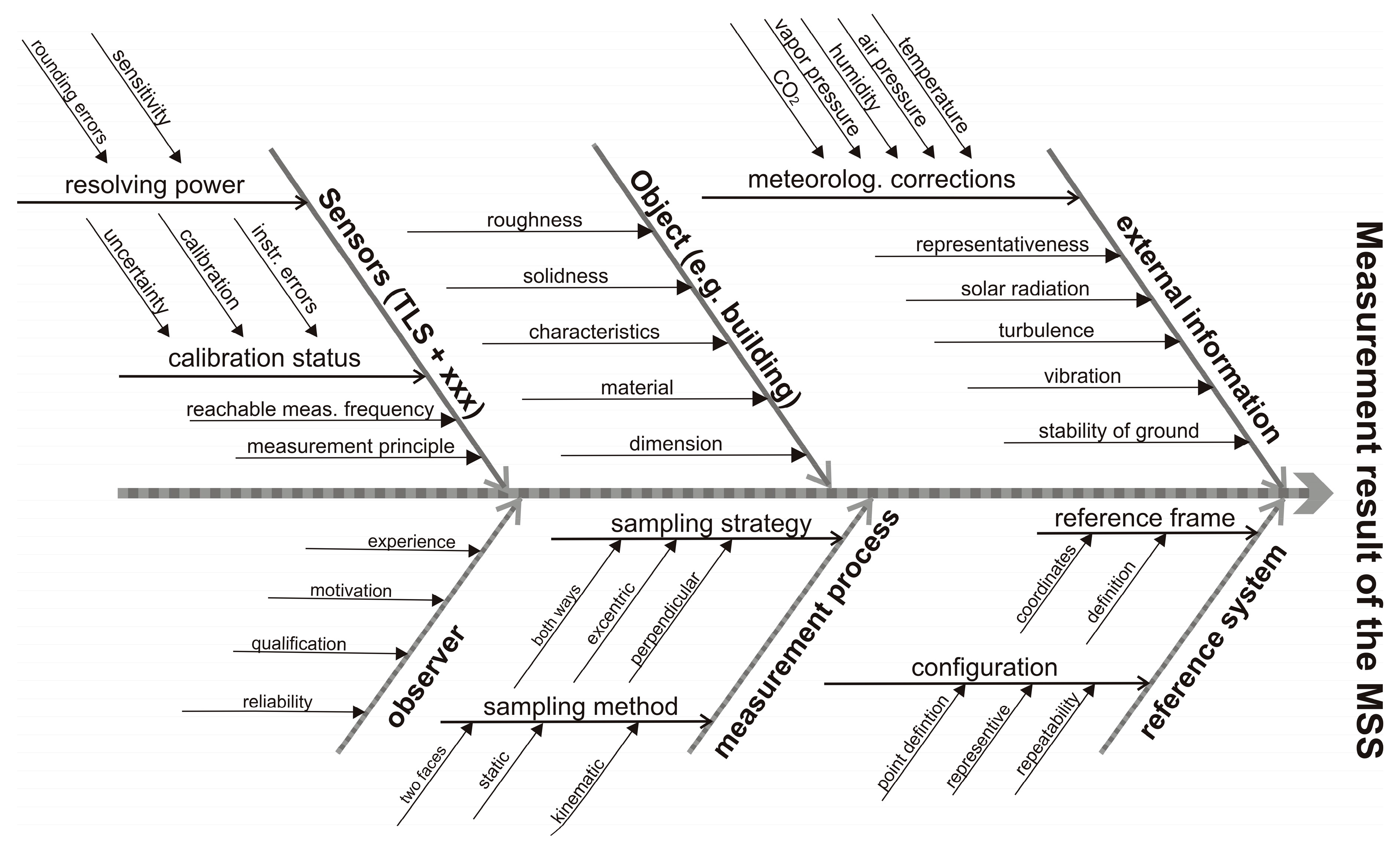
:1. Introduction
- Sensor-specific influences
- Influences dependent on the captured object
- Influences caused by the configuration of the measurement or the measurement process
- External influences like the atmospheric conditions
2. Environment/Infrastructure
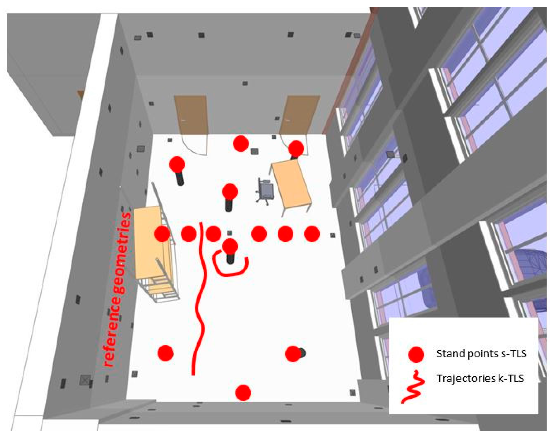
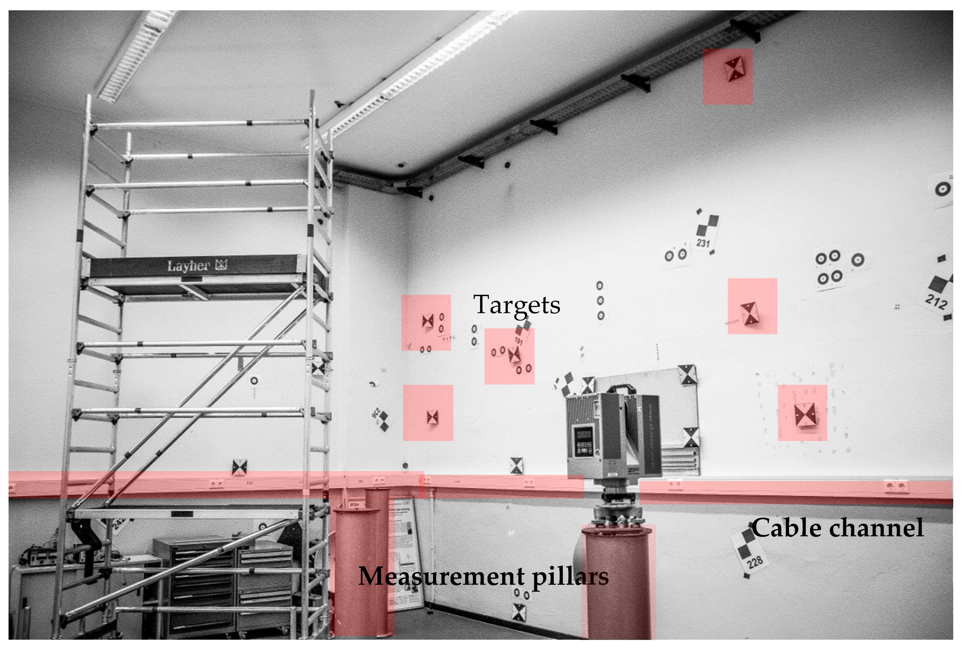
2.1. 3D-Laboratory and 3D-Reference Frame
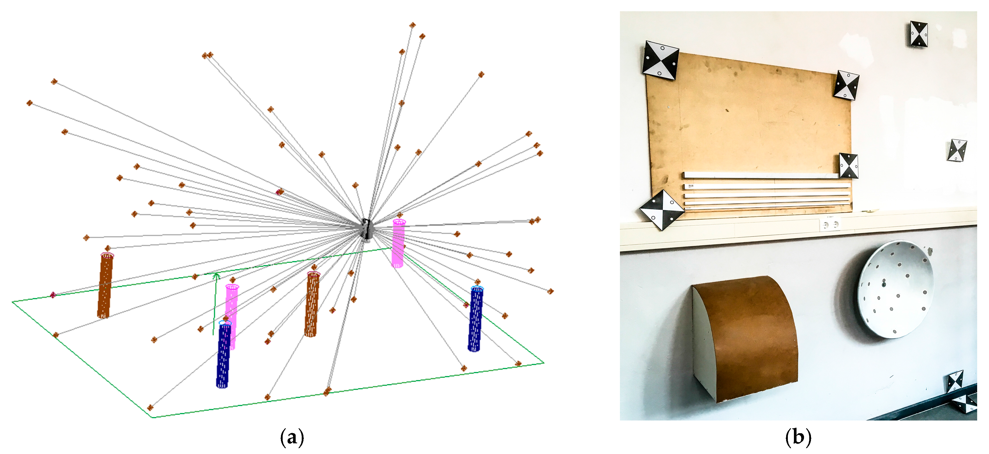
2.2. Reference Geometries
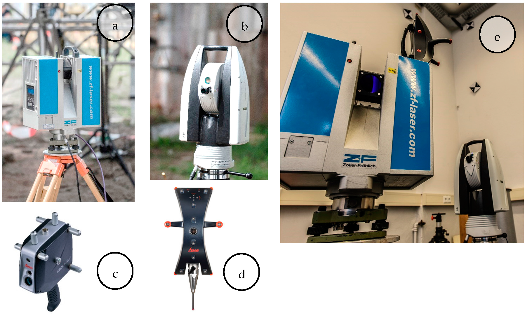
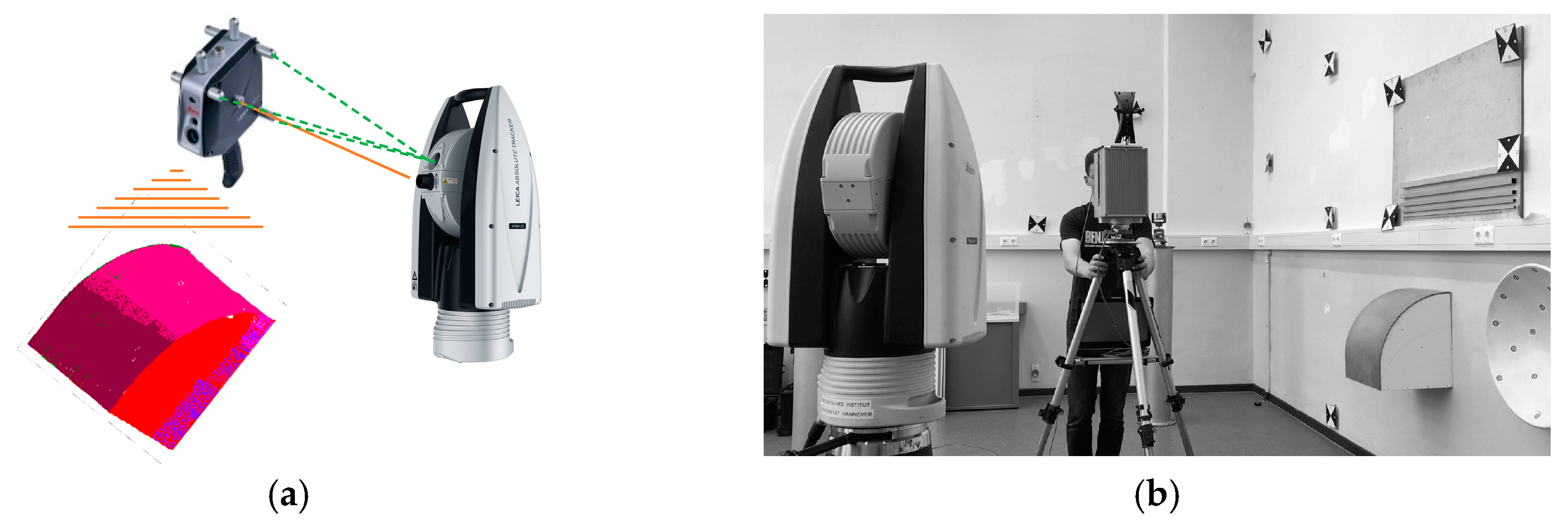
2.3. Sensors with Superordinate Accuracy/Investigated Sensors and MSS
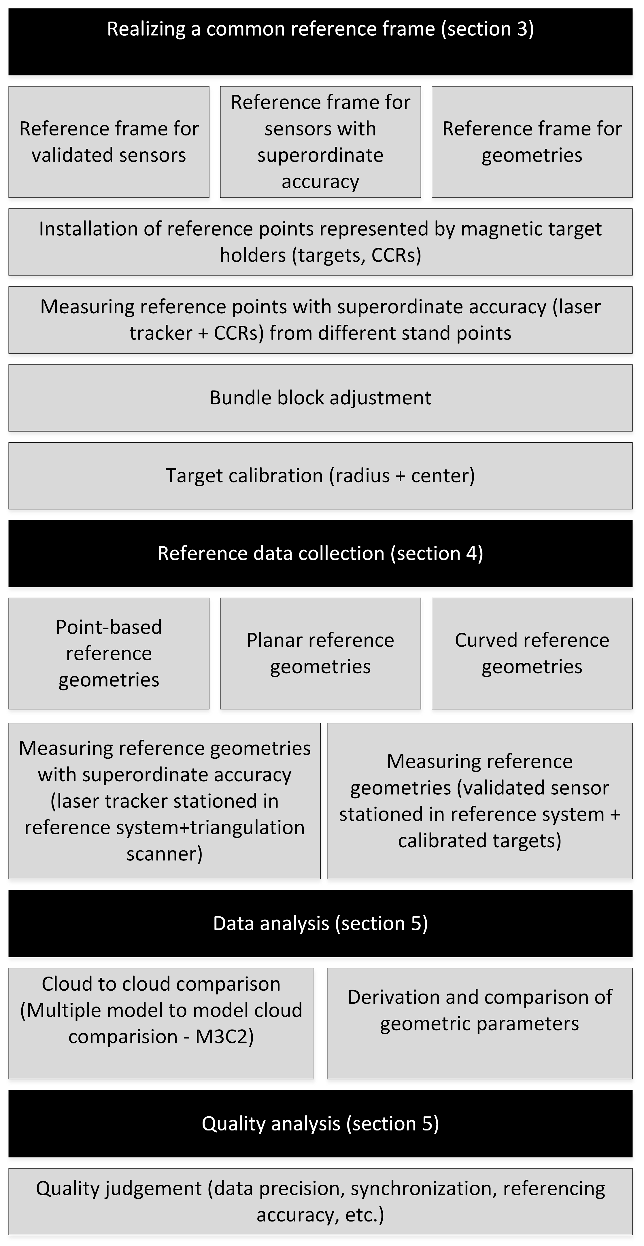
3. Realization of a Reference Frame for Sensors and Geometries
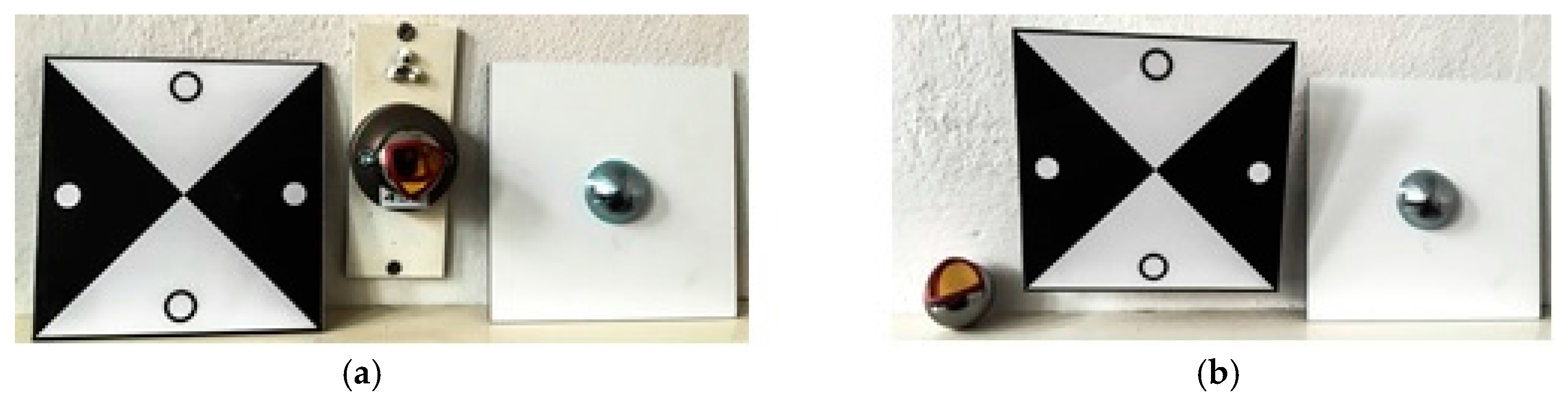
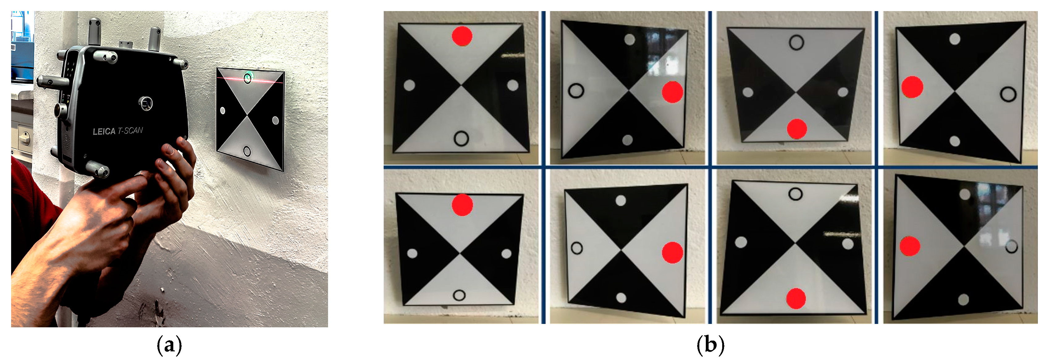
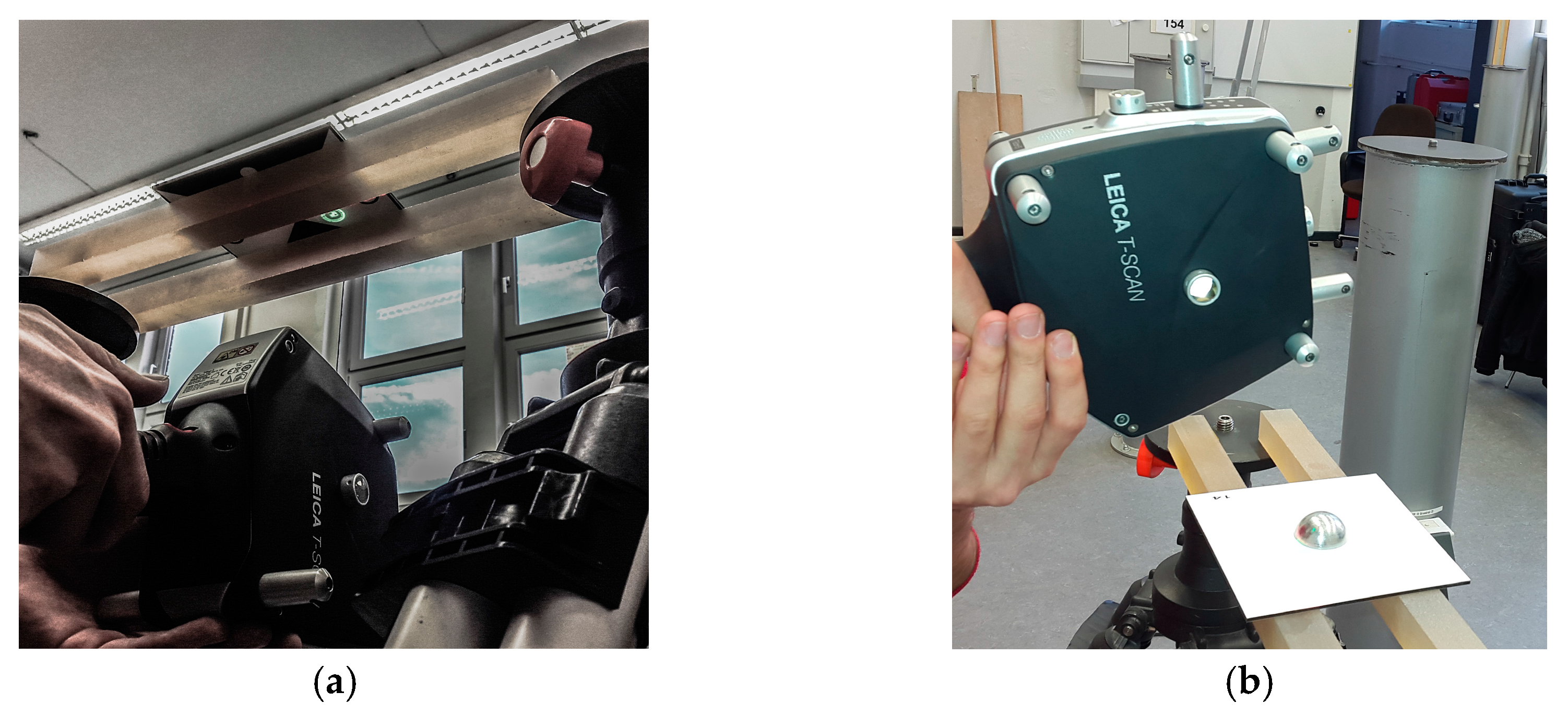
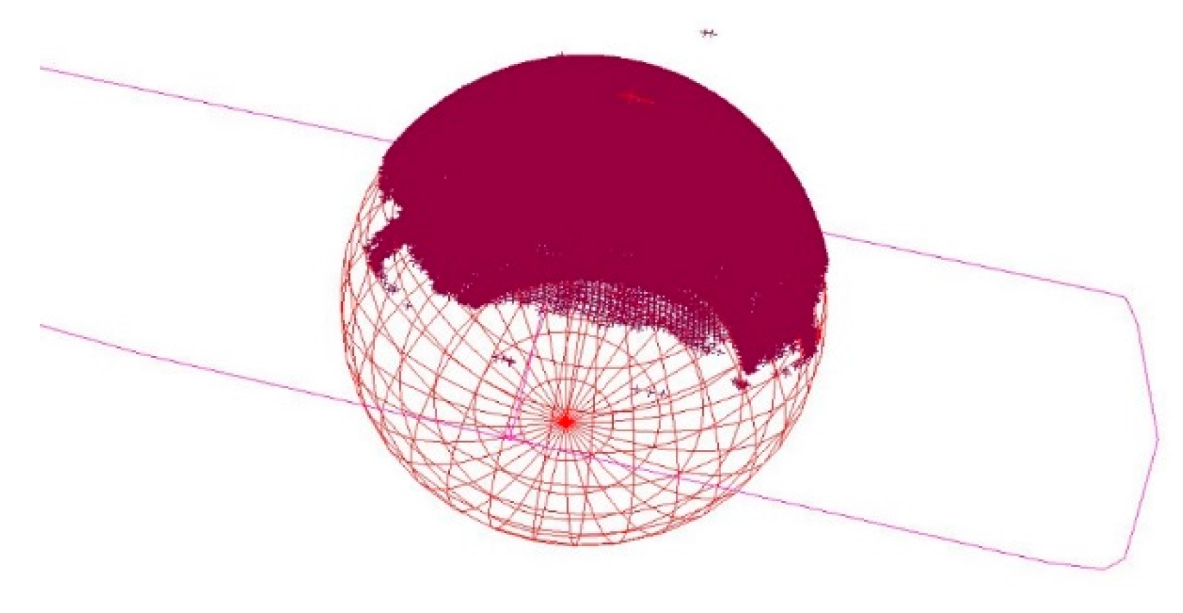
3.1. Calibration of the Target Centre
3.2. Calibration of the Target Radius
4. Data Sampling for Areal Reference Geometries
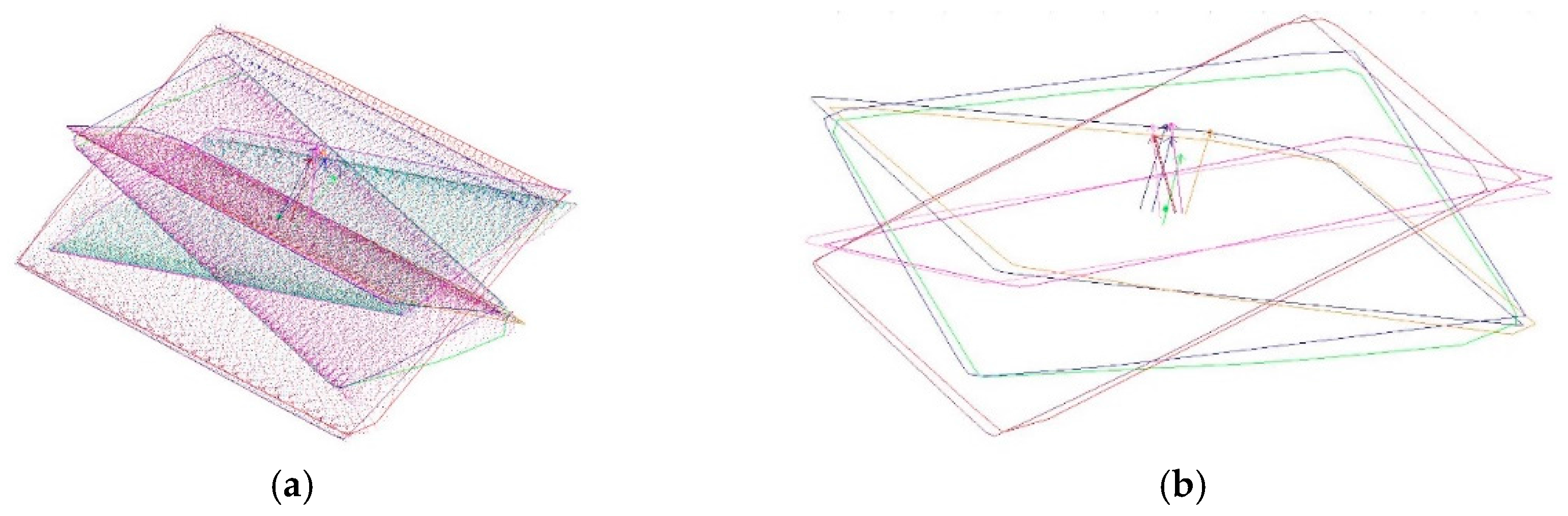
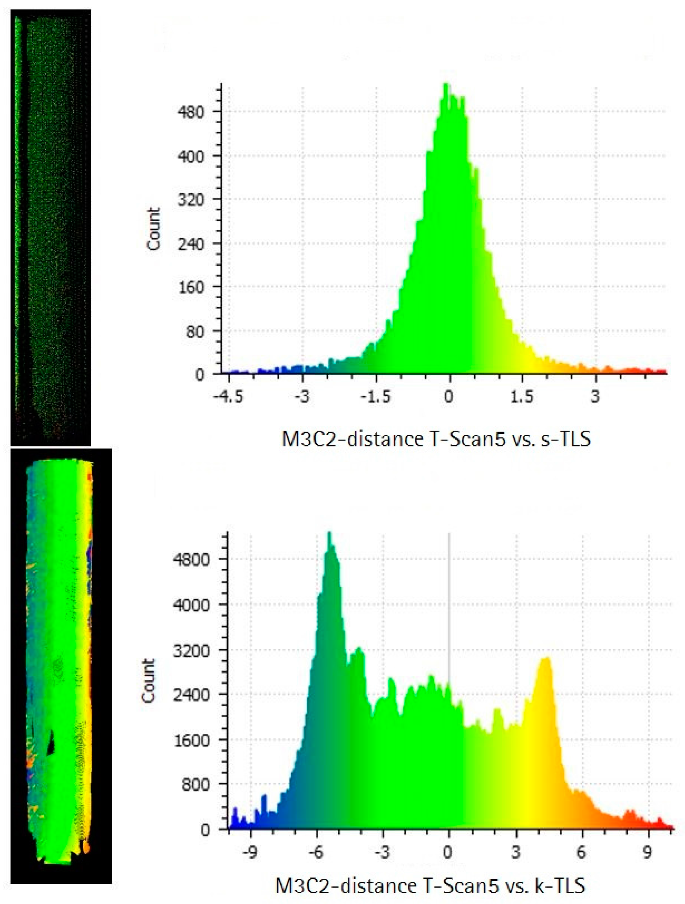
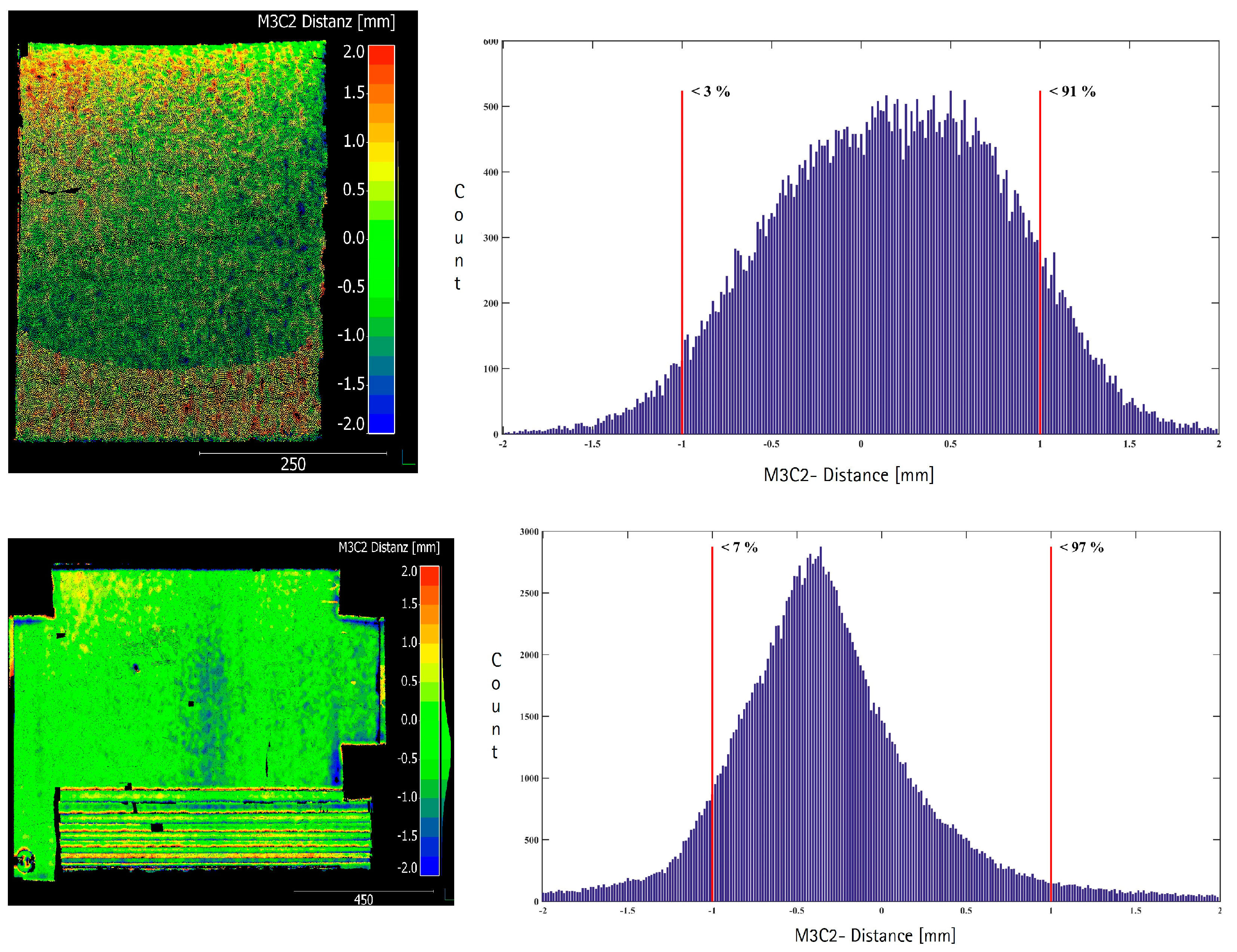
- The direct point cloud to point cloud comparison using the M3C2-algorithm (multiple scale model to model cloud comparison, [31].
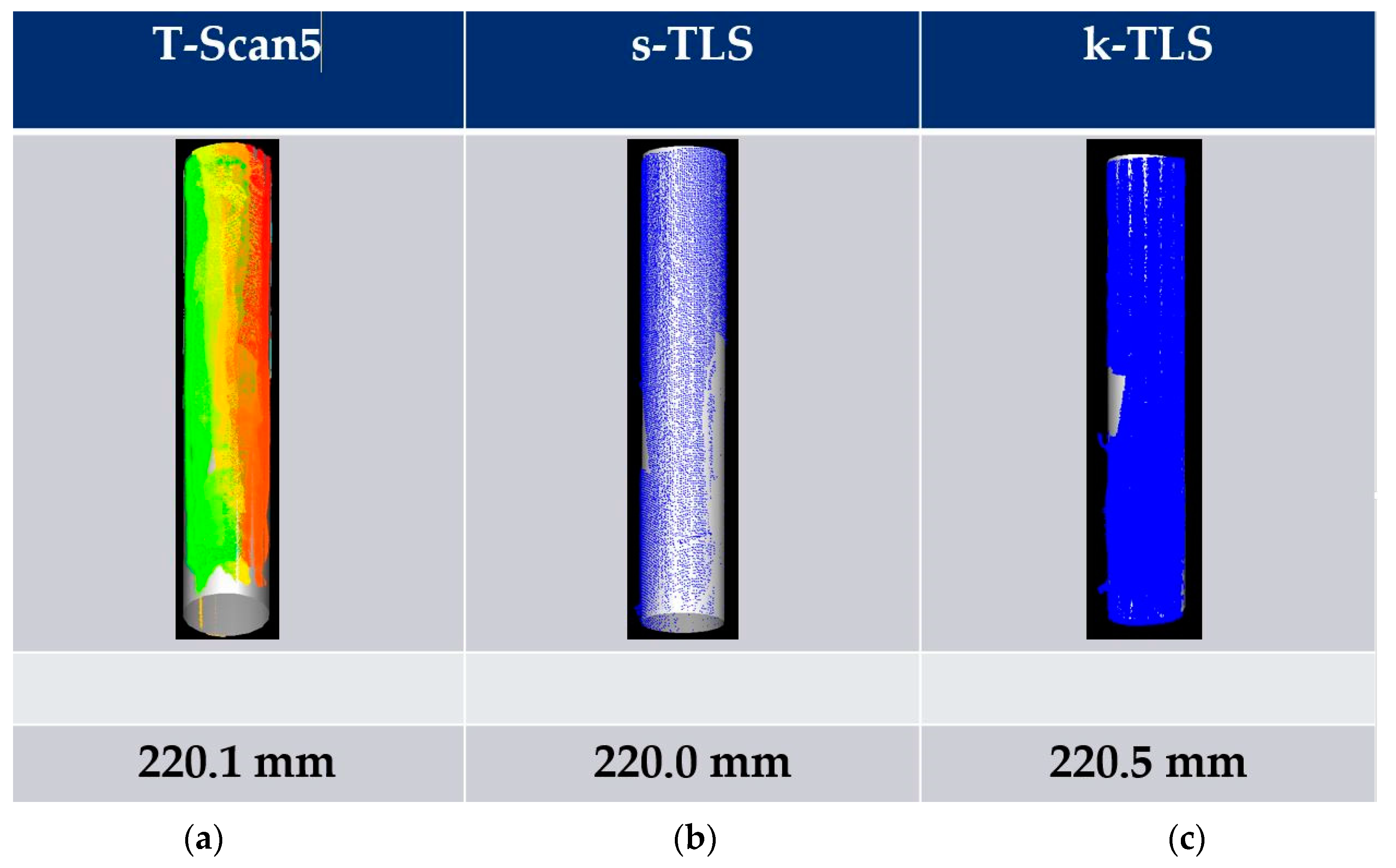
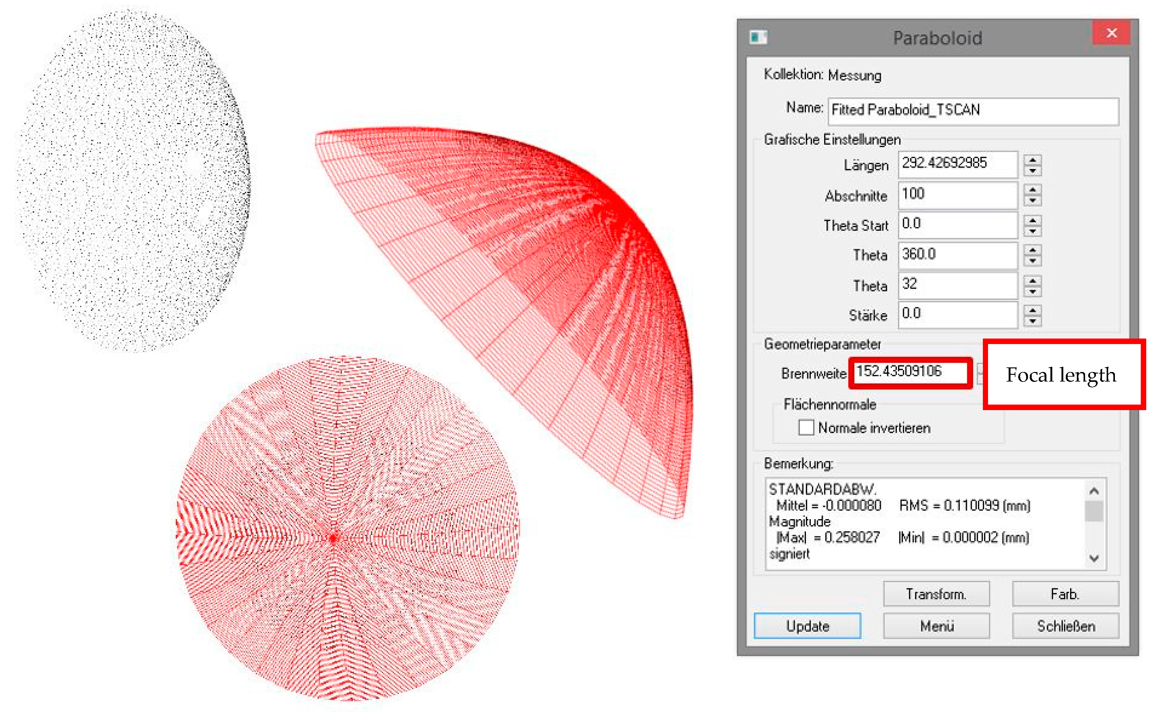
- The comparison of geometrical parameters derived from the point clouds, like the cylinders diameter or the focal length of the paraboloid.
5. Data Analysis
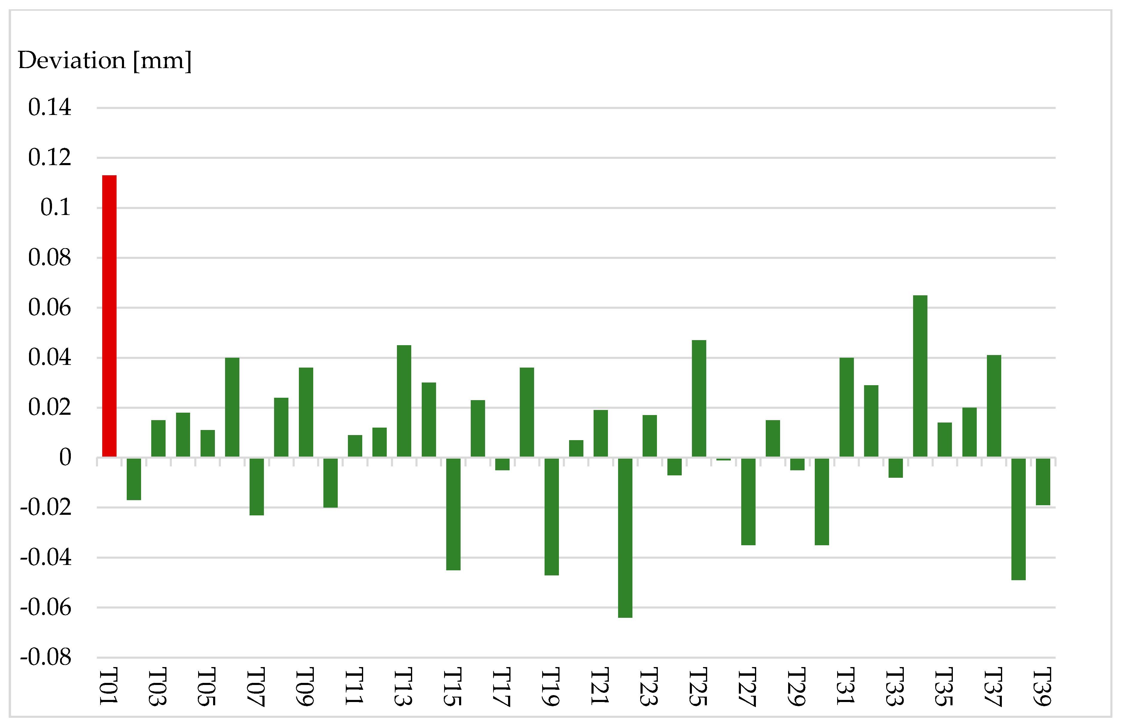
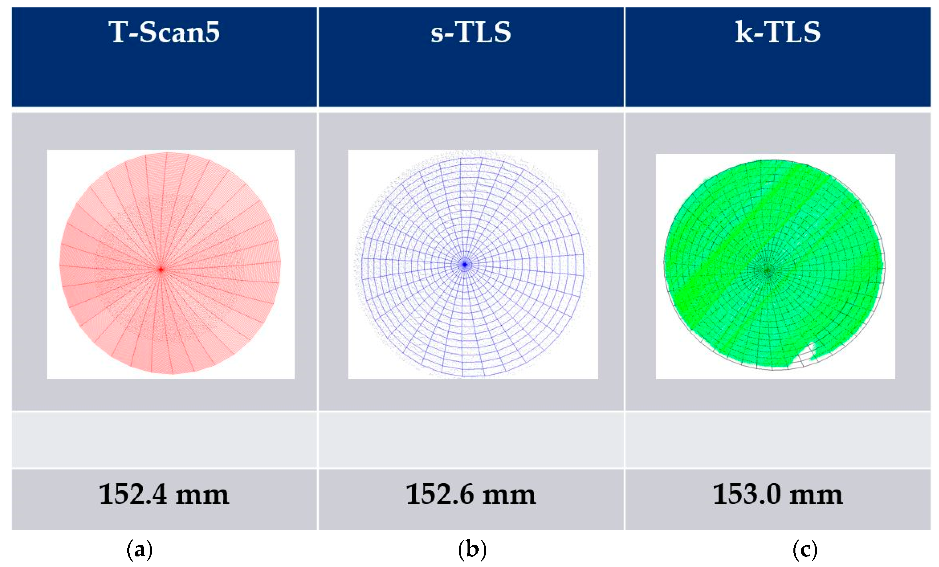
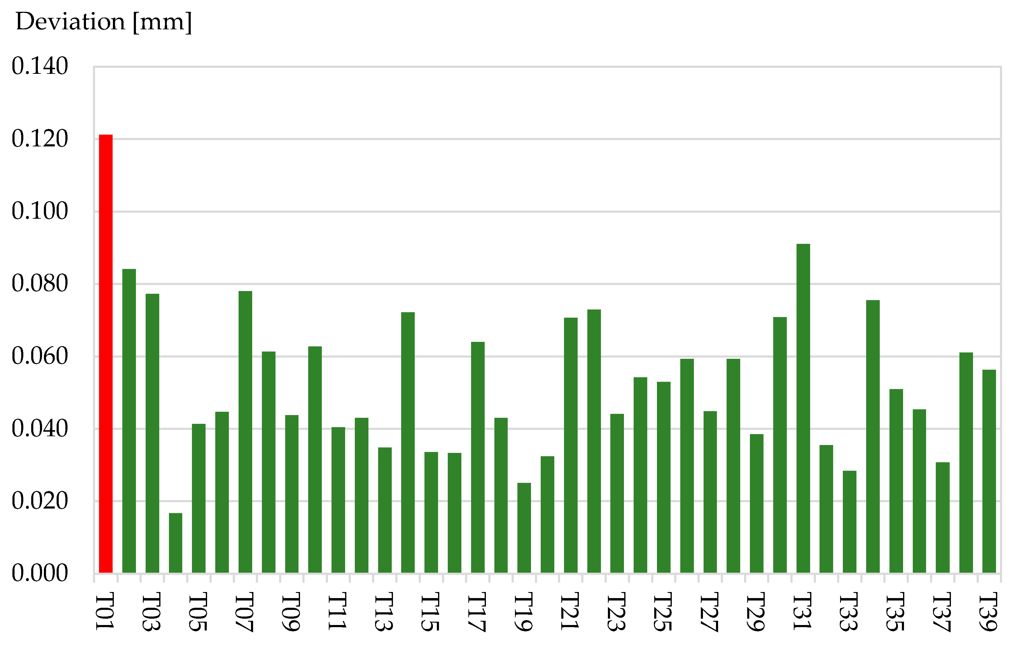
5.1. Comparison of Geometrical Parameters
5.2. Cloud to Cloud Comparison Using the M3C2-Algorithm
6. Conclusions and Outlook
Acknowledgments
Author Contributions
Conflicts of Interest
References
- Hennes, M.; Heister, H. Neuere aspekte zur Definition und zum Gebrauch von Genauigkeitsmaßen in der Ingenieurgeodäsie. Allg. Vermess. Nachr. (AVN) 2007, 114, 375–383. (In German) [Google Scholar]
- JCGM 100: Evaluation of Measurement Data—Guide to the Expression of Uncertainty in Measurement (GUM 1995 with Minor Corrections, ISO/IEC Guide 98-3) Version 2008; Joint Committee for Guides in Metrology (JCGM/WG 1). 2008.
- Koch, K.-R. Determining uncertainties of correlated measurements by Monte Carlo simulations applied to laserscanning. J. Appl. Geod. 2008, 2, 139–147. [Google Scholar] [CrossRef]
- Alkhatib, H.; Neumann, I.; Kutterer, H. Uncertainty modeling of random and systematic errors by means of Monte Carlo and fuzzy techniques. J. Appl. Geod. 2009, 3, S67–S79. [Google Scholar] [CrossRef]
- Paffenholz, J.-A.; Alkhatib, H.; Stenz, U.; Neumann, I. Aspekte der Qualitätssicherung von Multi-Sensor-Systemen. Allg. Vermess. Nachr. (AVN) 2017, 124, 79–91. (In German) [Google Scholar]
- Wujanz, D. Terrestrial Laser Scanning for Geodetic Deformation Monitoring. Ph.D. Thesis, German Geodetic Commission, Munich, Germany, 2016. [Google Scholar]
- Wujanz, D.; Burger, M.; Mettenleiter, M.; Neitzel, F. An intensity-based stochastic model for terrestrial laser scanners. ISPRS J. Photogramm. Remote Sens. 2017, 125, 146–155. [Google Scholar] [CrossRef]
- Hennes, M. Konkurrierende Genauigkeitsmaße—Potential und Schwächen aus der Sicht des Anwenders. Allg. Vermess. Nachr. 2007, 114, 136–146. [Google Scholar]
- Neitzel, F. Gemeinsame Bestimmung von Ziel-, Kippachsenfehler und Exzentrizität der Zielachse am Beispiel des Laserscanners Zoller+Fröhlich Imager 5003; Herbert Wichmann Verlag: Heidelberg, Germany, 2006. (In German) [Google Scholar]
- Neitzel, F. Untersuchung des Achssystems und des Taumelfehlers terrestrischer Laserscanner mit tachymetrischem Messprinzip. In Terrestrisches Laser-Scanning (TLS 2006); Wißner-Verlag: Augsburg, Germany, 2006; pp. 15–34. (In German) [Google Scholar]
- Gordon, B. Determining the Uncertainties Concerning Terrestrial Laser Scanner Measurements. Ph.D. Thesis, Technische Universität Darmstadt, Darmstadt, Germany, 2008. [Google Scholar]
- Holst, C.; Nothnagel, A.; Blome, M.; Becker, P.; Eichborn, M.; Kuhlmann, H. Improved area-based deformation analysis of a radio telescope’s main reflector based on terrestrial laser scanning. J. Appl. Geod. 2015, 9, 1–14. [Google Scholar] [CrossRef]
- Lichti, D.D. Ray-Tracing Method for Deriving Terrestrial Laser Scanner Systematic Errors. J. Surv. Eng. 2017, 6016005. [Google Scholar] [CrossRef]
- Zámečníková, M.; Wieser, A.; Woschitz, H.; Ressl, C. Influence of surface reflectivity on reflectorless electronic distance measurement and terrestrial laser scanning. J. Appl. Geod. 2014, 8. [Google Scholar] [CrossRef]
- Schulz, T.; Ingensand, H. Terrestrial laser scanning—Investigations and applications for high precision scanning. In Proceedings of the FIG Working Week, Athens, Greece, 22–27 May 2004. [Google Scholar]
- Soudarissanane, S.; Lindenbergh, R.; Menenti, M.; Teunissen, P.J.G. Scanning geometry: Influencing factor on the quality of terrestrial laser scanning points. ISPRS J. Photogramm. Remote Sens. 2011, 66, 389–399. [Google Scholar] [CrossRef]
- Zámečníková, M.; Neuner, H. Der Einfluss des Auftreffwinkels auf die reflektorlose Distanzmessung. In Terrestrisches Laserscanning 2014 (TLS 2014); Wißner-Verlag: Augsburg, Germany, 2014; pp. 69–85. (In German) [Google Scholar]
- Kauker, S.; Schwieger, V. First investigations for a synthetic covariance matrix for monitoring by terrestrial laser scanning. In Proceedings of the 3rd Joint International Symposium on Deformation Monitoring, Vienna, Austria, 30 April–1 March 2016. [Google Scholar]
- Schmitt, A. Combining laser tracker and laser scanner data. In Integration of Point- and Area-Wise Geodetic Monitoring for Structures and Natural Objects; Karpik, A.P., Schwieger, V., Novitskaya, A., Lerke, O., Eds.; Siberian State Academy of Geodesy: Novosibirsk, Russia, 2014. [Google Scholar]
- Neuner, H.; Holst, C.; Kuhlmann, H. Overview on current modelling strategies of point clouds for deformation analysis. Allg. Vermess. Nachr. (AVN) 2016, 123, 328–339. [Google Scholar]
- Holst, C.; Neuner, H.; Wieser, A.; Wunderlich, T.A.; Kuhlmann, H. Calibration of Terrestrial Laser Scanners. Allg. Vermess. Nachr. (AVN) 2016, 123, 147–157. [Google Scholar]
- Hexagon Metrology. Leica T-Scan 5 Brochure; Hexagon Metrology: Unterentfelden, Switzerland, 2014. [Google Scholar]
- Hexagon Metrology. Leica Absolute Tracker AT960 Brochure; Hexagon Metrology: Unterentfelden, Switzerland, 2015. [Google Scholar]
- Zoller+Fröhlich GmbH. Technical Data IMAGER 5006; Version 1.0.5; Zoller+Fröhlich GmbH: Wangen im Allgäu, Germany, 2007. (In German) [Google Scholar]
- Hartmann, J.; Paffenholz, J.-A.; Strübing, T.; Neumann, I. Determination of Position and Orientation of LiDAR Sensors on Multisensor Platforms. J. Surv. Eng. 2017, 143. [Google Scholar] [CrossRef]
- Schulz, T. Calibration of a Terrestrial Laser Scanner for Engineering Geodesy. Ph.D. Thesis, ETH Zürich Inst. f. Geodäsie u. Photogrammetrie, Zurich, Switzerland, 2007. [Google Scholar]
- Vennegeerts, H.; Martin, J.; Kutterer, H.; Becker, M. Validation of a kinematic laserscanning system. J. Appl. Geod. 2008, 2, 79–84. [Google Scholar] [CrossRef]
- Strübing, T.; Neumann, I. Positions- und Orientierungsschätzung von LIDAR-Sensoren auf Multisensorplattformen. Z. Geod. Geoinf. Landmanag. 2013, 138, 210–221. [Google Scholar]
- Hartmann, J.; Marschel, L.; Dorndorf, A.; Paffenholz, J.-A. Ein objektraumbasierter und durch Referenzmessungen gestützter Kalibrierprozess für ein k-TLS-basiertes Multi-Sensor-System. Allg. Vermess. Nachr. (AVN) 2017, 124, 3–10. (In German) [Google Scholar]
- Holst, C.; Schmitz, B.; Kuhlmann, H. TLS-basierte Deformationsanalyse unter Nutzung von Standardsoftware. In Terrestrisches Laserscanning 2016 (TLS 2016); Wißner-Verlag: Augsburg, Germany, 2016; pp. 39–58. (In German) [Google Scholar]
- Lague, D.; Brodu, N.; Leroux, J. Accurate 3D comparison of complex topography with terrestrial laser scanner. Application to the Rangitikei canyon (N-Z). ISPRS J. Photogramm. Remote Sens. 2013, 82, 10–26. [Google Scholar] [CrossRef]


| Component | Functions | Requirements |
|---|---|---|
| Laboratory | Environment for reference frame and reference geometries. | Stable environmental conditions (temperature, atmospheric pressure, humidity), geometric stability of the reference points. |
| Reference frame | Reproducibility of the measurements, common reference frame for the participating sensors, referencing of the sensors and geometries. | Calibrated targets representing the reference points, targets must be measurable by all participating sensors (point based, area based sensors), reference points must be stable, coordinates of the reference points with higher accuracy than tested sensors, reference points have to be well distributed. |
| Reference geometries | Investigation of different influence factors (distance, incident angle, material, colour) for point based and area based sensors. | Different materials (wood, metal, plastic), different colours (white, …, black), different dimensions (point, plane, sphere), different shapes and curvatures. |
| Reference sensors | Providing data with superordinate accuracy. | Higher level of accuracy than the tested sensors (sub mm). |
| Investigated sensors/MSS | Sampling reference geometries (volume, area or point based). | No special requirements. |
| Reference Geometry | Shape | Material | Colour | Sensitive Influence Factors |
|---|---|---|---|---|
 | cuboids | 5× metal, 1× wood | silver, light brown | resolution |
 | curved surface | wood | dark brown | incidence angle (vertical) |
 | paraboloid | metal | white | incidence angle (horizontal and vertical) |
 | cylinder | metal | silver | incidence angle (horizontal), synchronization, referencing |
 | cuboid (cable channel) | plastic | grey | distance, incidence angle (horizontal and vertical) |
| Sensor | Accuracy |
|---|---|
| Leica AT960 LR | ±15 µm + 6 µm/m (angle accuracy, maximum permissible error (MPE)) |
| ±0.5 µm/m (distance accuracy Absolute Interferometer, MPE) | |
| Leica T-Probe | Ux,y,z = ±30 µm + 10 µm/m uncertainty up to 25m, (MPE) |
| Leica T-Scan 5 | Ux,y,z = ±60 µm under 8.5 m (MPE) |
| UP = ± 80 μm + 3 μm/m (2σ, uncertainty for plane surfaces) | |
| Z+F Imager 5006 | 0.007° rms (angle horizontal and vertical) |
| 1.2 mm rms (distance noise, 10 m, reflectivity black) | |
| 0.7 mm rms (distance noise, 10 m, reflectivity dark grey) | |
| 0.4 mm rms (distance noise, 10 m, reflectivity white) |
| Reference Geometrie | Point Cloud (T-Scan 5) | Number of Points |
|---|---|---|
 |  | 12,500,000 |
 |  | 6,500,000 |
 |  | 7,500,000 |
 |  | 17,000,000 |
© 2017 by the authors. Licensee MDPI, Basel, Switzerland. This article is an open access article distributed under the terms and conditions of the Creative Commons Attribution (CC BY) license (http://creativecommons.org/licenses/by/4.0/).
Share and Cite
Stenz, U.; Hartmann, J.; Paffenholz, J.-A.; Neumann, I. A Framework Based on Reference Data with Superordinate Accuracy for the Quality Analysis of Terrestrial Laser Scanning-Based Multi-Sensor-Systems. Sensors 2017, 17, 1886. https://doi.org/10.3390/s17081886
Stenz U, Hartmann J, Paffenholz J-A, Neumann I. A Framework Based on Reference Data with Superordinate Accuracy for the Quality Analysis of Terrestrial Laser Scanning-Based Multi-Sensor-Systems. Sensors. 2017; 17(8):1886. https://doi.org/10.3390/s17081886
Chicago/Turabian StyleStenz, Ulrich, Jens Hartmann, Jens-André Paffenholz, and Ingo Neumann. 2017. "A Framework Based on Reference Data with Superordinate Accuracy for the Quality Analysis of Terrestrial Laser Scanning-Based Multi-Sensor-Systems" Sensors 17, no. 8: 1886. https://doi.org/10.3390/s17081886