Characterization of Quadratic Nonlinearity between Motion Artifact and Acceleration Data and its Application to Heartbeat Rate Estimation


Abstract
:1. Introduction
2. Datasets and Performance Measure
3. Signal Model
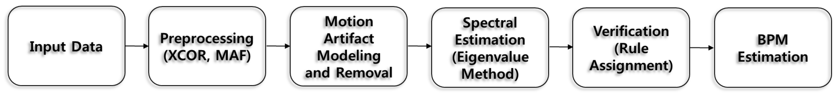
4. Approaches
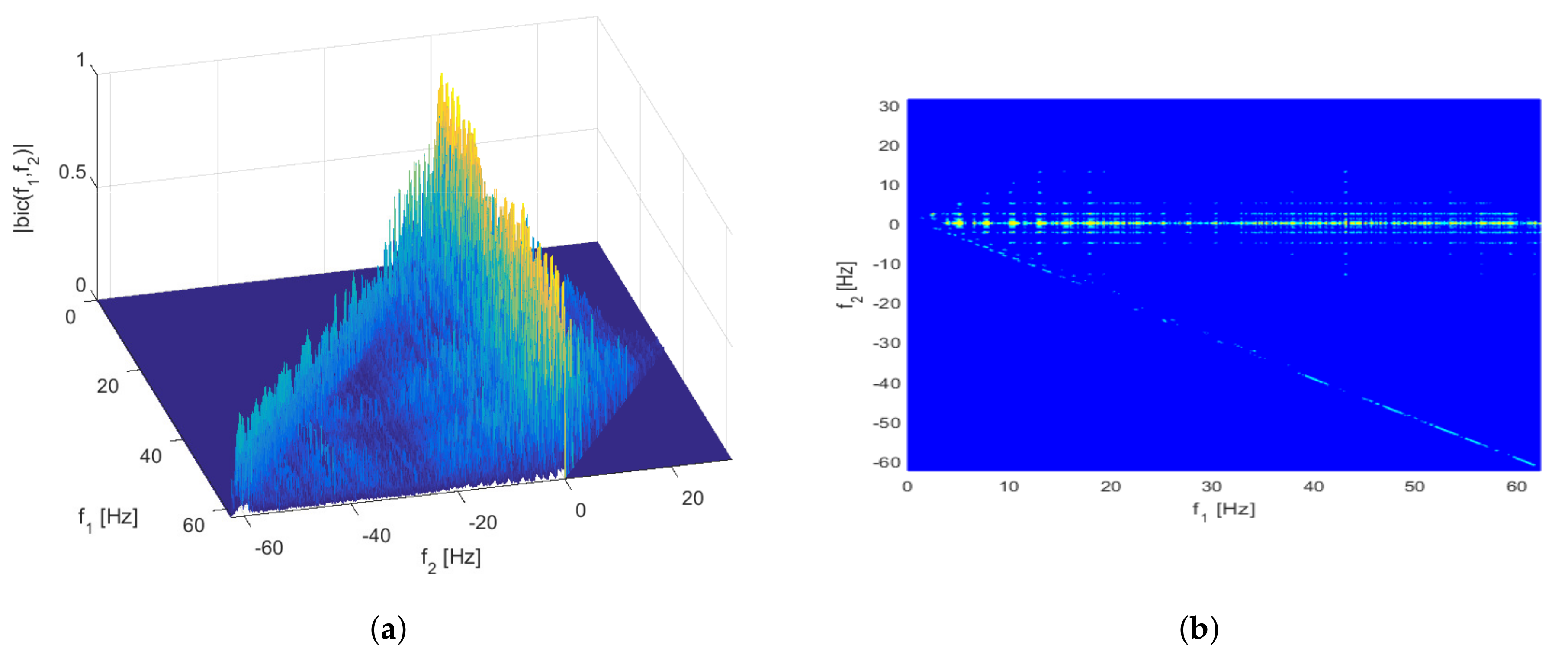
4.1. Cross Bicoherence Test
4.2. A Second-Order Volterra Filter
4.3. Heartbeat Rate Estimation Using PPG Signals
5. Results
5.1. Application of Cross Bicoherence Test
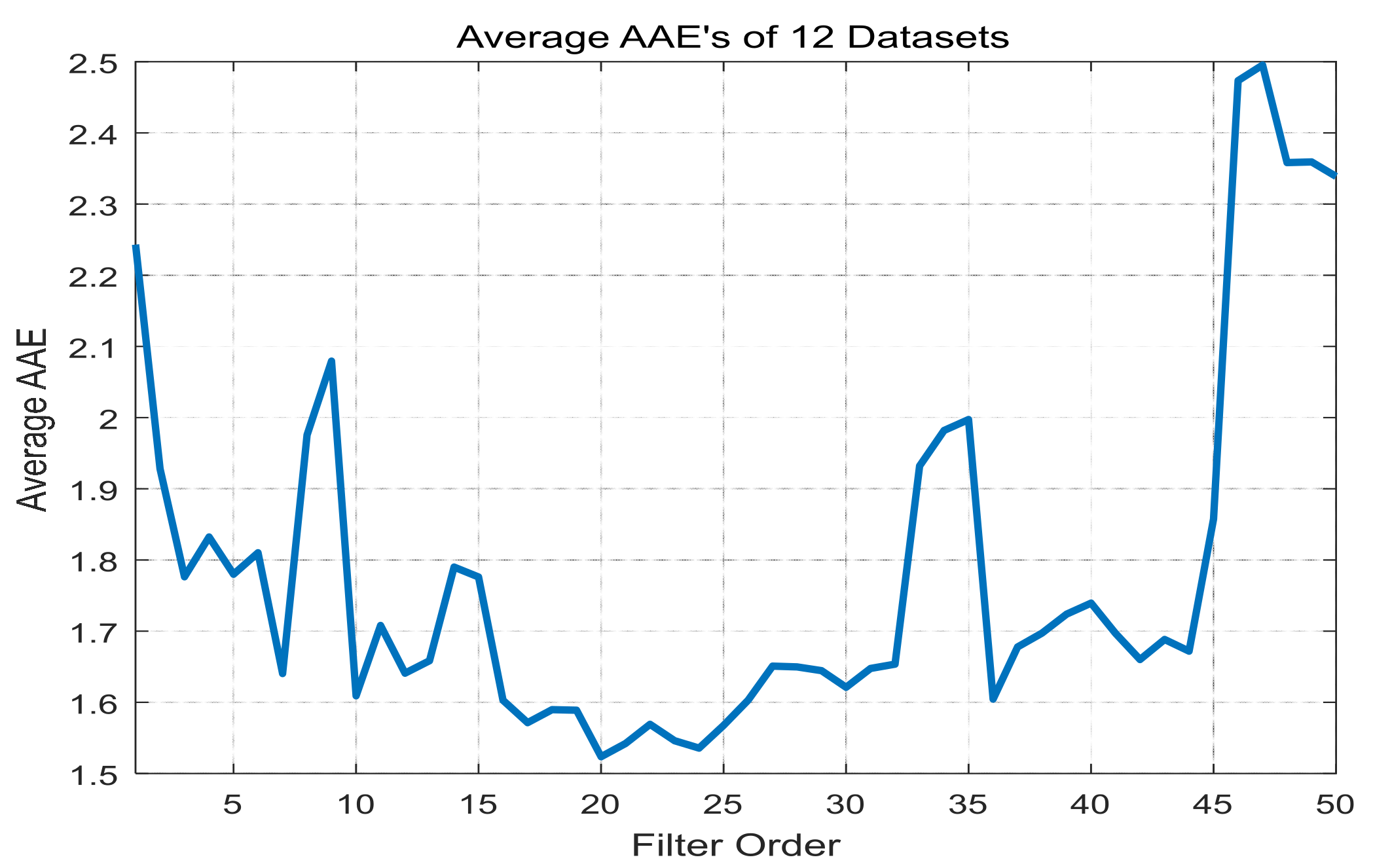
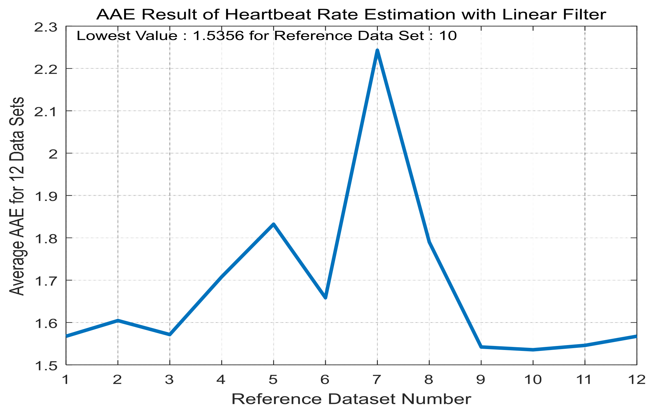
5.2. Application to Heartbeat Rate Estimation
5.3. Model Cross Validation
6. Conclusions
Acknowledgments
Author Contributions
Conflicts of Interest
References
- Bassett, D.R.; Troiano, R.P.; McClain, J.J.; Wolff, D.L. Accelerometer-based physical activity: Total volume per day and standardized measures. Med. Sci. Sports Exerc. 2015, 47, 833–838. [Google Scholar] [CrossRef] [PubMed]
- Vanhelst, J.; Béghin, L.; Duhamel, A.; Bergman, P.; Sjöström, M.; Gottrand, F. Comparison of uniaxial and triaxial accelerometry in the assessment of physical activity among adolescents under free-living conditions: The HELENA study. BMC Med. Res. Methodol. 2012, 12, 26. [Google Scholar] [CrossRef] [PubMed]
- Allen, J. Photoplethysmography and its application in clinical physiological measurement. Physiol. Meas. 2007, 28, R1. [Google Scholar] [CrossRef] [PubMed]
- Kamal, A.; Harness, J.; Irving, G.; Mearns, A. Skin photoplethysmography: A review. Comput. Methods Programs Biomed. 1989, 28, 257–269. [Google Scholar] [CrossRef]
- Tamura, T.; Maeda, Y.; Sekine, M.; Yoshida, M. Wearable Photoplethysmographic Sensors-Past and Present. Electronics 2014, 3, 282–302. [Google Scholar] [CrossRef]
- Relente, A.; Sison, L. Characterization and adaptive filtering of motion artifacts in pulse oximetry using accelerometers. In Engineering in Medicine and Biology, Proceedings of the Second Joint, 24th Annual Conference and the Annual Fall Meeting of the Biomedical Engineering Society EMBS/BMES Conference, Houston, TX, USA, 23–26 October 2002; IEEE: Piscataway, NJ, USA, 2002; Volume 2, pp. 1769–1770. [Google Scholar]
- Shimazaki, T.; Hara, S.; Okuhata, H.; Nakamura, H.; Kawabata, T. Cancellation of Motion Artifact Induced by Exercise for PPG-Based Heart Rate Sensing. In Proceedings of the IEEE 36th Annual International Conference on Engineering in Medicine and Biology Society (EMBC), Chicago, IL, USA, 26–30 August 2014; pp. 3216–3219. [Google Scholar]
- Yousefi, R.; Nourani, M.; Ostadabbas, S.; Panahi, I. A motion-tolerant adaptive algorithm for wearable photoplethysmographic biosensors. IEEE J. Biomed. Health Inform. 2014, 18, 670–681. [Google Scholar] [CrossRef] [PubMed]
- Ram, M.R.; Madhav, K.V.; Krishna, E.H.; Komalla, N.R.; Reddy, K.A. A Novel Approach for Motion Artifact Reduction in PPG Signals Based on AS-LMS Adaptive Filter. IEEE Trans. Instrum. Meas. 2012, 61, 1445–1457. [Google Scholar] [CrossRef]
- Kim, S.H.; Ryoo, D.W.; Bae, C. Adaptive Noise Cancellation Using Accelerometers for the PPG Signal from Forehead. In Proceedings of the IEEE 29th Annual International Conference on Engineering in Medicine and Biology Society (EMBS 2007), Lyon, France, 22–26 August 2007; IEEE: Piscataway, NJ, USA, 2007; pp. 2564–2567. [Google Scholar]
- Han, H.; Kim, J. Artifacts in wearable photoplethysmographs during daily life motions and their reduction with least mean square based active noise cancellation method. Comput. Biol. Med. 2012, 42, 387–393. [Google Scholar] [CrossRef] [PubMed]
- Lee, C.M.; Zhang, Y.T. Reduction of Motion Artifacts from Photoplethysmographic Recordings Using a Wavelet Denoising Approach. In Proceedings of the IEEE EMBS Asian-Pacific Conference on Biomedical Engineering, Kyoto, Japan, 20–22 October 2003; IEEE: Piscataway, NJ, USA, 2003; pp. 194–195. [Google Scholar]
- Raghuram, M.; Madhav, K.V.; Krishna, E.H.; Reddy, K.A. Evaluation of Wavelets for Reduction of Motion Artifacts in Photoplethysmographic Signals. In Proceedings of the 10th International Conference on Information Sciences Signal Processing and their Applications (ISSPA), Kuala Lumpur, Malaysia, 10–13 May 2010; IEEE: Piscataway, NJ, USA, 2010; pp. 460–463. [Google Scholar]
- Naraharisetti, K.; Bawa, M.; Tahernezhadi, M. Comparison of Different Signal Processing Methods for Reducing Artifacts from Photoplethysmograph Signal. In Proceedings of the 2011 IEEE International Conference on Electro/Information Technology (EIT), Mankato, MN, USA, 15–17 May 2011; IEEE: Piscataway, NJ, USA, 2011; pp. 1–8. [Google Scholar]
- Foo, J.Y.A. Comparison of wavelet transformation and adaptive filtering in restoring artefact-induced time-related measurement. Biomed. Signal Process. Control 2006, 1, 93–98. [Google Scholar] [CrossRef]
- Lee, B.; Han, J.; Baek, H.J.; Shin, J.H.; Park, K.S.; Yi, W.J. Improved elimination of motion artifacts from a photoplethysmographic signal using a Kalman smoother with simultaneous accelerometry. Physiol. Meas. 2010, 31, 1585. [Google Scholar] [CrossRef] [PubMed]
- Seyedtabaii, S.; Seyedtabaii, L. Kalman filter based adaptive reduction of motion artifact from photoplethysmographic signal. World Acad. Sci. Eng. Technol. 2008, 37, 173–176. [Google Scholar]
- Krishnan, R.; Natarajan, B.; Warren, S. Two-stage approach for detection and reduction of motion artifacts in photoplethysmographic data. IEEE Trans. Biomed. Eng. 2010, 57, 1867–1876. [Google Scholar] [CrossRef] [PubMed]
- Yao, J.; Warren, S. A Short Study to Assess the Potential of Independent Component Analysis for Motion Artifact Separation in Wearable Pulse Oximeter Signals. IEEE Int. Conf. Eng. Med. Biol. Soc. 2005, 4, 3585–3588. [Google Scholar]
- Kim, B.S.; Yoo, S.K. Motion artifact reduction in photoplethysmography using independent component analysis. IEEE Trans. Biomed. Eng. 2006, 53, 566–568. [Google Scholar] [CrossRef] [PubMed]
- Reddy, K.; Kumar, V. Motion Artifact Reduction in Photoplethysmographic Signals Using Singular Value Decomposition. In Proceedings of the IEEE Instrumentation and Measurement Technology Conference, Warsaw, Poland, 1–3 May 2007; IEEE: Piscataway, NJ, USA, 2007; pp. 1–4. [Google Scholar]
- Zhang, Z.; Pi, Z.; Liu, B. TROIKA: A General Framework for Heart Rate Monitoring Using Wrist-Type Photoplethysmographic Signals During Intensive Physical Exercise. IEEE Trans. Biomed. Eng. 2015, 62, 522–531. [Google Scholar] [CrossRef] [PubMed]
- Zhang, Y.; Liu, B.; Zhang, Z. Combining ensemble empirical mode decomposition with spectrum subtraction technique for heart rate monitoring using wrist-type photoplethysmography. Biomed. Signal Process. Control 2015, 21, 119–125. [Google Scholar] [CrossRef]
- Ye, Y.; Cheng, Y.; He, W.; Hou, M.; Zhang, Z. Combining Nonlinear Adaptive Filtering and Signal Decomposition for Motion Artifact Removal in Wearable Photoplethysmography. IEEE Sens. J. 2016, 16, 7133–7141. [Google Scholar] [CrossRef]
- Hinich, M.J. Testing for gaussianity and linearity of a stationary time series. J. Time Ser. Anal. 1982, 3, 169–176. [Google Scholar] [CrossRef]
- Nikias, C.L.; Raghuveer, M.R. Bispectrum estimation: A digital signal processing framework. In Proceedings of the IEEE; IEEE: Piscataway, NJ, USA, 1987; Volume 75, pp. 869–891. [Google Scholar]
- Choudhury, M.S.; Shah, S.L.; Thornhill, N.F. Diagnosis of poor control-loop performance using higher-order statistics. Automatica 2004, 40, 1719–1728. [Google Scholar] [CrossRef]
- Arlot, S.; Celisse, A. A survey of cross-validation procedures for model selection. Stat. Surv. 2010, 4, 40–79. [Google Scholar] [CrossRef]
- Zhang, Z. Undergraduate Students Compete in the IEEE Signal Processing Cup: Part 3 [SP Education]. IEEE Signal Process. Mag. 2015, 32, 113–116. [Google Scholar] [CrossRef]
- Sun, B.; Zhang, Z. Photoplethysmography-Based Heart Rate Monitoring Using Asymmetric Least Squares Spectrum Subtraction and Bayesian Decision Theory. IEEE Sens. J. 2015, 15, 7161–7168. [Google Scholar] [CrossRef]
- Salehizadeh, S.; Dao, D.; Bolkhovsky, J.; Cho, C.; Mendelson, Y.; Chon, K. A novel time-varying spectral filtering algorithm for reconstruction of motion artifact corrupted heart rate signals during intense physical activities using a wearable photoplethysmogram sensor. Sensors 2016, 16, 10. [Google Scholar] [CrossRef]
- Yousefi, R.; Nourani, M.; Panahi, I. Adaptive Cancellation of Motion Artifact in Wearable Biosensors. In Proceedings of the IEEE 2012 Annual International Conference on Engineering in Medicine and Biology Society (EMBC), San Diego, CA, USA, 28 August–1 September 2012; pp. 2004–2008. [Google Scholar]
- Kim, S.; Lee, J.; Kang, H.; Ohn, B.; Baek, G.; Jung, M.; Im, S. Heart rate monitoring using motion artifact modeling with MISO filters. J. Inst. Electron. Inf. Eng. 2015, 52, 18–26. [Google Scholar] [CrossRef]
- Peng, F.; Liu, H.; Wang, W. A comb filter based signal processing method to effectively reduce motion artifacts from photoplethysmographic signals. Physiol. Meas. 2015, 36, 2159. [Google Scholar] [CrossRef] [PubMed]
- Renevey, P.; Vetter, R.; Krauss, J.; Celka, P.; Depeursinge, Y. Wrist-located pulse detection using IR signals, activity and nonlinear artifact cancellation. In Proceedings of the IEEE 23rd Annual International Conference on Engineering in Medicine and Biology Society, Istanbul, Turkey, 25–28 October 2001; IEEE: Piscataway, NJ, USA, 2001; Volume 3, pp. 3030–3033. [Google Scholar]
- Bouten, C.; Westerterp, K.; Verduin, M.; Janssen, J. Assessment of energy expenditure for physical activity using a triaxial accelerometer. Med. Sci. Sports Exerc. 1994, 23, 21–27. [Google Scholar] [CrossRef]
- Im, S.; Powers, E.J. A sparse third-order orthogonal frequency-domain Volterra-like model. J. Frankl. Inst. 1996, 333, 385–412. [Google Scholar] [CrossRef]
- Haykin, S.S. Adaptive Filter Theory; Pearson Education India: Taramani, India, 2008. [Google Scholar]
- Stoica, P.; Moses, R.L. Spectral Analysis of Signals; Pearson Prentice Hall: Upper Saddle River, NJ, USA, 2005; Volume 452. [Google Scholar]
- Marple, S.L. A Tutorial Overview of Modern Spectral Estimation. In Proceedings of the 1989 International Conference on Acoustics, Speech, and Signal Processing (ICASSP-89), Glasgow, UK, 23–26 May 1989; IEEE: Piscataway, NJ, USA, 1989; Volume 4, pp. 2152–2157. [Google Scholar]
- Marple, S.L. Digital Spectral Analysis: With Applications; Prentice-Hall: Englewood Cliffs, NJ, USA, 1987; Volume 5. [Google Scholar]
- Harris, F. On the Use of Windows for Harmonic Analysis with the Discrete Fourier Transform. Proc. IEEE 1978, 66, 51–83. [Google Scholar] [CrossRef]


| Dataset | x-axis | y-axis | z-axis | ||||||||
|---|---|---|---|---|---|---|---|---|---|---|---|
| (Hz) | (Hz) | Coherence | (Hz) | (Hz) | Coherence | (Hz) | (Hz) | Coherence | |||
| data 1 | 5.859 | −2.808 | 0.562 | 4.395 | −1.465 | 0.484 | 8.789 | −5.859 | 0.556 | ||
| data 2 | 2.808 | −1.343 | 0.731 | 6.958 | −5.493 | 0.722 | 2.808 | −1.343 | 0.713 | ||
| data 3 | 2.808 | −1.343 | 0.577 | 2.808 | −1.343 | 0.603 | 8.545 | −7.080 | 0.578 | ||
| data 4 | 4.639 | −2.686 | 0.359 | 43.457 | −41.138 | 0.396 | 43.579 | 0.000 | 0.854 | ||
| data 5 | 49.927 | 0.610 | 0.687 | 5.615 | −4.150 | 0.675 | 61.401 | 0.000 | 0.742 | ||
| data 6 | 5.005 | −3.784 | 0.654 | 5.005 | −3.784 | 0.618 | 8.789 | −7.568 | 0.613 | ||
| data 7 | 5.127 | −3.784 | 0.526 | 2.686 | −1.343 | 0.485 | 2.564 | −1.221 | 0.502 | ||
| data 8 | 11.719 | −8.789 | 0.720 | 60.913 | 0.000 | 0.857 | 7.324 | −4.395 | 0.724 | ||
| data 9 | 5.981 | −4.883 | 0.574 | 2.319 | −1.221 | 0.677 | 57.739 | 0.000 | 0.757 | ||
| data 10 | 3.662 | 0.122 | 0.766 | 12.939 | 0.122 | 0.935 | 6.470 | −0.366 | 0.912 | ||
| data 11 | 4.517 | −2.930 | 0.697 | 58.838 | −0.122 | 0.919 | 7.446 | −5.859 | 0.660 | ||
| data12 | 4.517 | −1.465 | 0.722 | 5.981 | −2.930 | 0.697 | 59.204 | 0.000 | 0.766 | ||
| Dataset | x-axis | y-axis | z-axis | ||||||||
|---|---|---|---|---|---|---|---|---|---|---|---|
| (Hz) | (Hz) | Coherence | (Hz) | (Hz) | Coherence | (Hz) | (Hz) | Coherence | |||
| data1 | 3.052 | −1.587 | 0.568 | 4.517 | −3.052 | 0.521 | 7.446 | −5.981 | 0.595 | ||
| data2 | 1.465 | 1.343 | 0.657 | 57.495 | 0.000 | 0.698 | 6.958 | −4.150 | 0.641 | ||
| data3 | 3.784 | −2.563 | 0.506 | 2.441 | −1.221 | 0.481 | 7.690 | −6.470 | 0.507 | ||
| data4 | 5.737 | −4.272 | 0.631 | 4.273 | −2.808 | 0.642 | 43.579 | 0.000 | 0.854 | ||
| data5 | 49.927 | −0.610 | 0.688 | 2.808 | −1.343 | 0.664 | 61.401 | 0.000 | 0.743 | ||
| data6 | 2.441 | −1.221 | 0.682 | 2.441 | −1.221 | 0.695 | 2.441 | −1.221 | 0.698 | ||
| data7 | 5.127 | −3.784 | 0.742 | 2.686 | −1.343 | 0.712 | 2.563 | −1.221 | 0.728 | ||
| data8 | 1.587 | 1.465 | 0.722 | 60.913 | 0.000 | 0.857 | 1.587 | 1.465 | 0.724 | ||
| data9 | 7.202 | −6.104 | 0.517 | 2.319 | −1.221 | 0.610 | 57.739 | 0.000 | 0.757 | ||
| data10 | 3.662 | 0.122 | 0.795 | 12.940 | −0.122 | 0.935 | 3.784 | 0.366 | 0.915 | ||
| data11 | 3.052 | −1.465 | 0.631 | 58.838 | 0.122 | 0.919 | 7.446 | −5.859 | 0.643 | ||
| data12 | 2.930 | −1.343 | 0.799 | 3.052 | −1.465 | 0.795 | 4.395 | −2.808 | 0.803 | ||
| Dataset | 1 | 2 | 3 | 4 | 5 | 6 | 7 | 8 | 9 | 10 | 11 | 12 |
|---|---|---|---|---|---|---|---|---|---|---|---|---|
| 25 | 36 | 17 | 11 | 4 | 13 | 1 | 14 | 21 | 24 | 23 | 25 | |
| AAE | 2.01 | 1.59 | 0.97 | 1.14 | 0.82 | 1.16 | 0.80 | 0.80 | 0.66 | 2.82 | 1.23 | 0.92 |
| Dataset | 1 | 2 | 3 | 4 | 5 | 6 | 7 | 8 | 9 | 10 | 11 | 12 |
|---|---|---|---|---|---|---|---|---|---|---|---|---|
| Axis | y | z | z | y | z | y | x | y | y | y | x | z |
| 17 | 29 | 14 | 9 | 3 | 10 | 1 | 10 | 2 | 5 | 25 | 13 | |
| 24 | 4 | 9 | 6 | 3 | 2 | 3 | 11 | 8 | 19 | 7 | 10 | |
| AAE | 1.61 | 1.48 | 0.93 | 1.10 | 0.83 | 1.08 | 0.84 | 0.74 | 0.63 | 2.19 | 1.16 | 0.79 |
© 2017 by the authors. Licensee MDPI, Basel, Switzerland. This article is an open access article distributed under the terms and conditions of the Creative Commons Attribution (CC BY) license (http://creativecommons.org/licenses/by/4.0/).
Share and Cite
Kim, S.; Im, S.; Park, T. Characterization of Quadratic Nonlinearity between Motion Artifact and Acceleration Data and its Application to Heartbeat Rate Estimation. Sensors 2017, 17, 1872. https://doi.org/10.3390/s17081872
Kim S, Im S, Park T. Characterization of Quadratic Nonlinearity between Motion Artifact and Acceleration Data and its Application to Heartbeat Rate Estimation. Sensors. 2017; 17(8):1872. https://doi.org/10.3390/s17081872
Chicago/Turabian StyleKim, Sunho, Sungbin Im, and Taehyung Park. 2017. "Characterization of Quadratic Nonlinearity between Motion Artifact and Acceleration Data and its Application to Heartbeat Rate Estimation" Sensors 17, no. 8: 1872. https://doi.org/10.3390/s17081872
APA StyleKim, S., Im, S., & Park, T. (2017). Characterization of Quadratic Nonlinearity between Motion Artifact and Acceleration Data and its Application to Heartbeat Rate Estimation. Sensors, 17(8), 1872. https://doi.org/10.3390/s17081872