For showing the potential of these approaches, a series of empirical tests was executed over real data and results achieved are presented and discussed in this section. The main question is as to which approach is more appropriate to reduce energy consumption and which is most suitable to maintain improved accuracy, while multidimensional data reading sensors were used.
4.2. Pearson Correlation and Linear Regression
The Pearson correlation coefficient (r) shows the magnitude of linear correlation between any two variables. This way, one can measure the strength of a correlation between variables across this coefficient, using the following interpretation: (1)
indicates a very strong correlation; (2)
r between
and
positive or negative indicates a strong correlation; and (3)
r below
indicates a moderate, weak or irrelevant correlation depending on the value of r [
25]. Thus, in our simulations, we consider the existence of correlation when the Pearson correlation coefficient (r) is greater than or equal to 0.7.
The Pearson correlation algorithm implementation considers that the independent variable will be the one that, having calculated the Pearson coefficients for all variables pair to pair, has the largest sum of coefficients greater than the minimum threshold (in our tests, the minimum threshold—called rPearsonMinimal—was set for the following values: 0.7, 0.8, 0.9, 0.95 and 0.99).
For each sensor in the network with the choice of the independent variable ’x’, we use ’x’ to calculate the linear regression coefficients ’a’ and ’b’ between ’x’ and each of the dependent variables of that sensor. Those variables that happened to have the Pearson correlation coefficient, relative to the independent variable, lower than the minimum threshold (0.7) are considered non-correlated variables. Thus, our solution can suppress the transmission of complete set of values (time series) from dependent variables, replacing the data set only for the respective linear regression coefficients (’a’ and ’b’), that will be used later to reconstruct the reading data from the dependent variables in sink node [
20]. This method has proved to be effective in filling the gaps of readings not made by sensor failures.
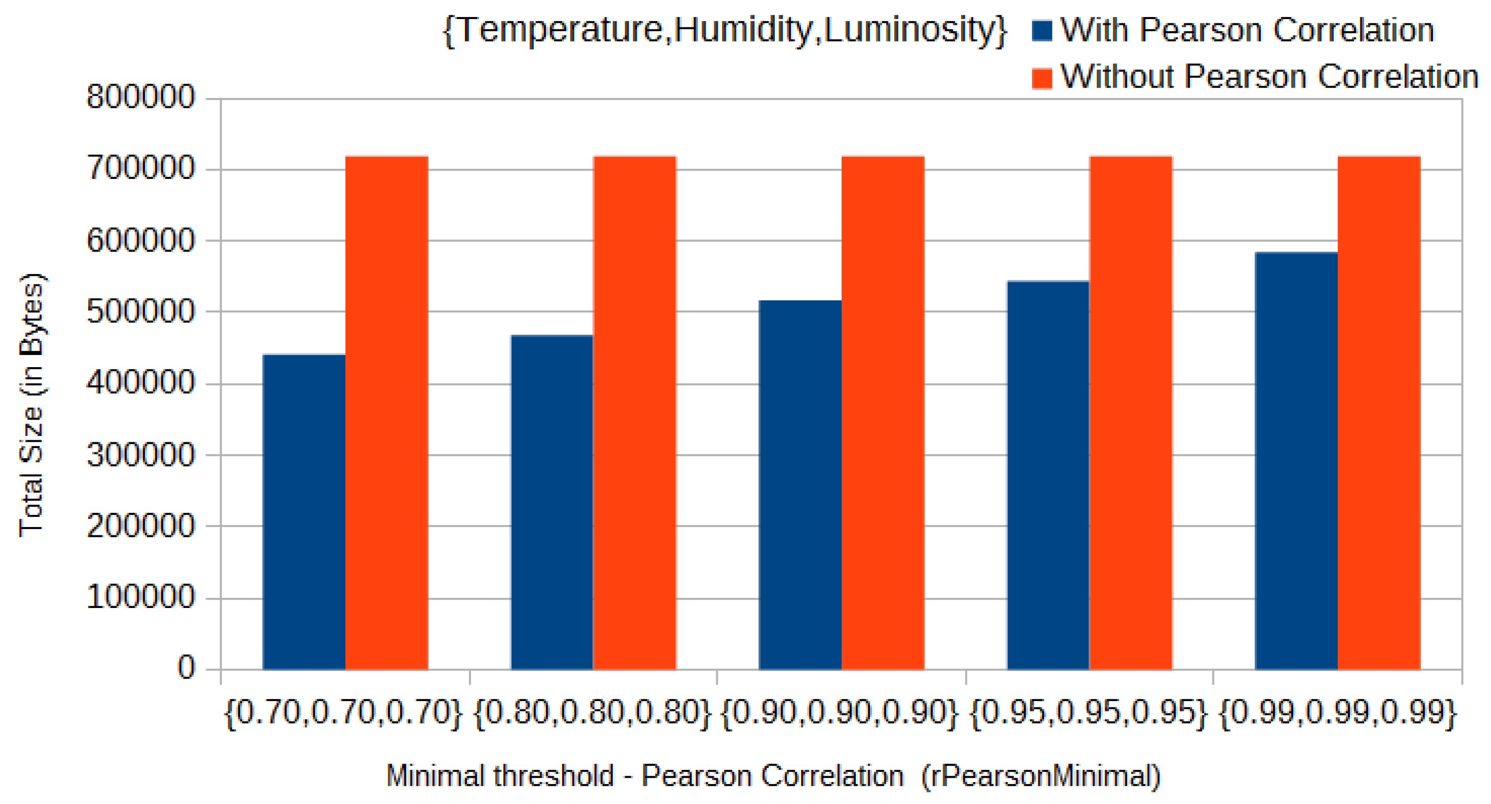
In our experiments, we used multidimensional data of the three physical phenomena. In that case, we considered an initial set of data of size equal to 70 readings from each of the sensed data types, to be sent by each sensor to the sink. Thus, with the Pearson correlation approach in use, the total size of messages sent by each sensor in the initial clustering phase decreased from 719 kB to 441 kB, that is, approximately
less network traffic in the initial phase, when using the three physical phenomena and with a threshold (
rPearsonMinimal) of 0.7 for all parameters (
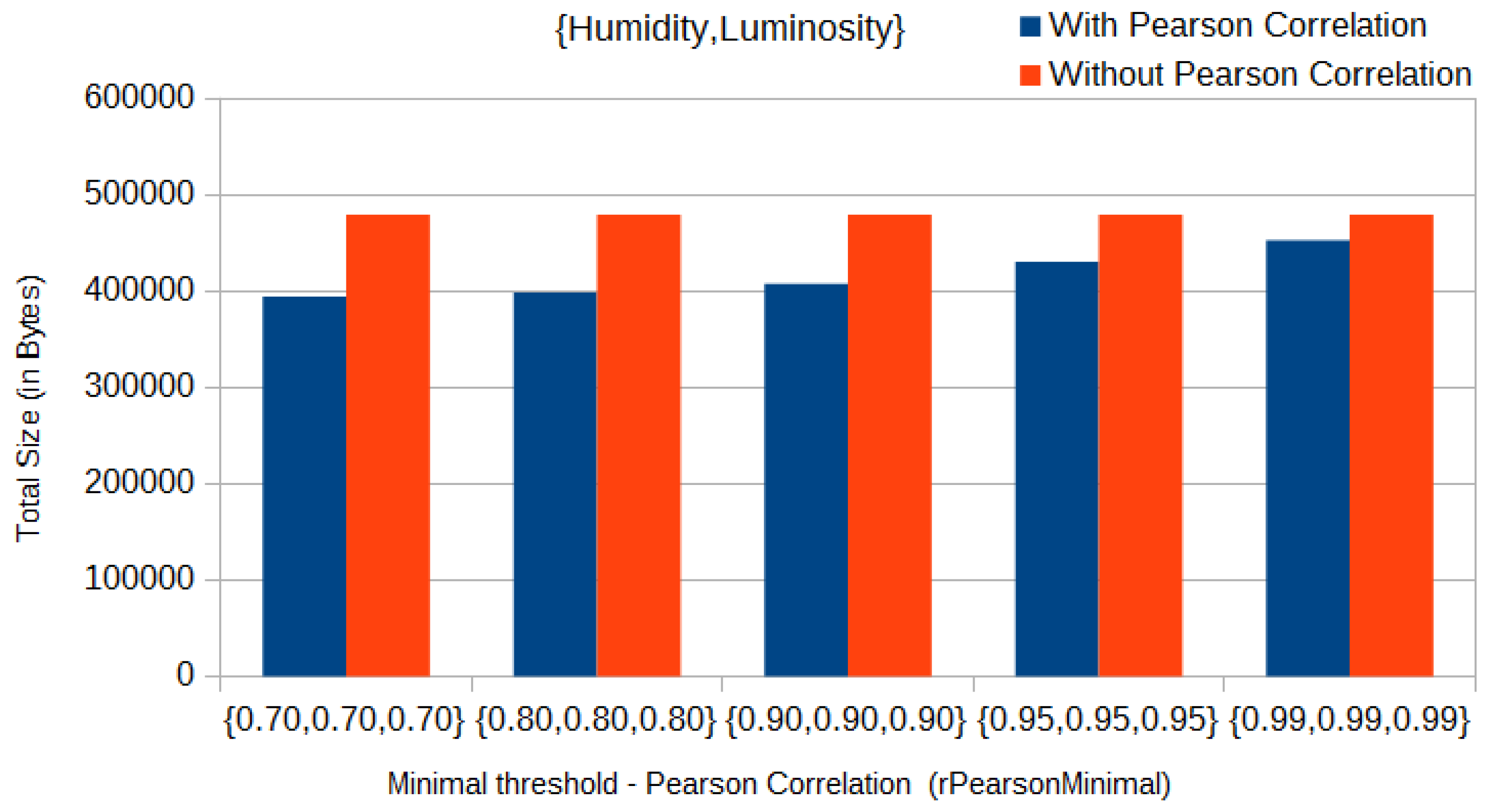
Figure 5). On the other hand, in a worst-case scenario, when using only humidity and luminosity and with a threshold (
rPearsonMinimal) of 0.99 for both parameters, the total size of messages sent in the initial clustering phase decreased from 479 kB to 452 kB (approximately
), as we can see in
Figure 6.
4.3. Initial Clustering: k-NN vs. MSM
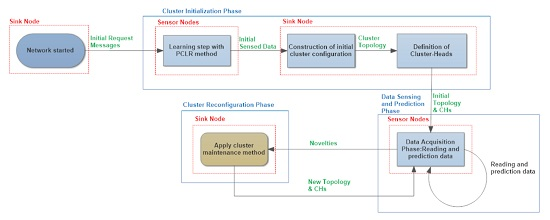
For multidimensional clusters initialization, the sink requests a certain amount of multidimensional sensed data from each sensor, which are sent to the sink. After receiving the requested data, the sink needs to classify each sensor into clusters (comparing multidimensional sensed data) and define the clustering configuration using multidimensional behavioral clustering of sensed data.
Fractal clustering is an incremental clustering technique. Hence, it is unable to initialize sensor clusters, requiring another algorithm able to do so.
In this work, we compared two different methods to define the initial clustering configuration: the general well-known k-nearest neighbors (k-NN) algorithm and the specific multidimensional similarity measure (MSM) algorithm. Parameter values for both algorithms were empirically defined. For k-NN, the k value was, empirically, fixed at 16, and the parameter values for MSM were and .
Our tests showed that the specialized MSM is better than the general k-nearest neighbors (k-NN), because keeping other parameters values, and using the FCM approach to cluster maintenance, we obtained the following results (see
Table 1) for the number of messages exchanged by the sensors, when we only changed the initial clustering method between k-NN and MSM.
Besides that,
Table 2 shows the RMSE for the FCM approach by using MSM compared with k-NN (NN with k = 2) as initial cluster algorithms for gathering
temperature data. Observe that using k–NN as initial cluster method, the RMSE is greater than same approach using MSM for all observed measurements.
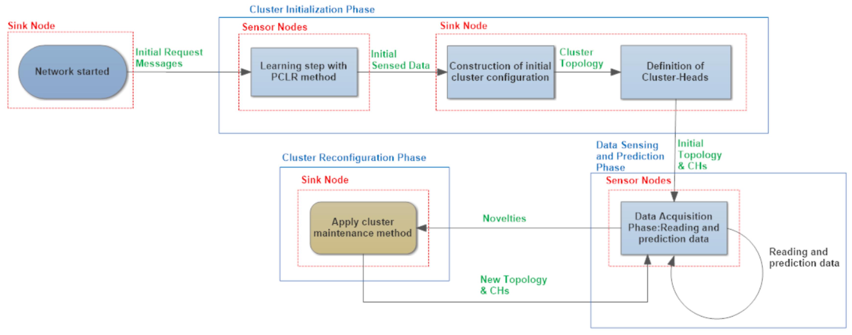
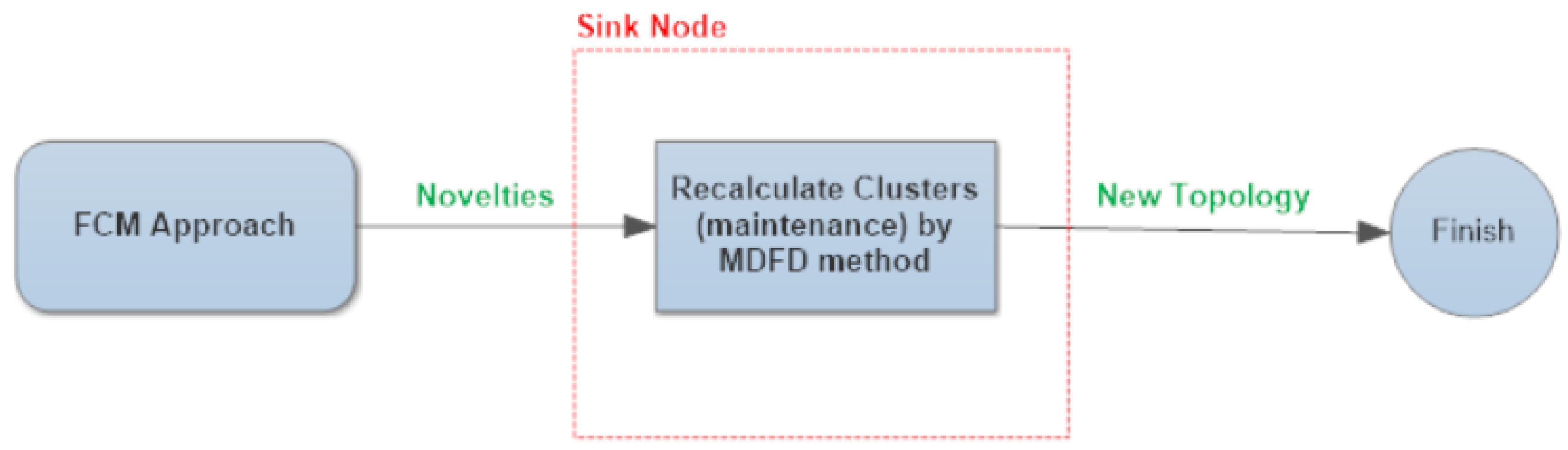
4.4. Maintenance of Clusters: FCM vs. SMM
With the goal of evaluating the proposed cluster maintenance approaches, two metrics have been employed: root-mean-square error (RMSE) to assess the precision of approaches, and amount of messages injected into the network. Temperature, humidity and luminosity were the dimensions used in the experiments, with the following combinations: (1) only humidity; (2) only luminosity; (3) temperature and humidity; and, finally; (4) temperature, humidity and luminosity.
Table 3 shows the generic simulation parameters and their corresponding values. The specific simulation parameters for SMM methods, with their values, are presented in
Table 4. In
Table 3, the number of initial readings parameter represents the amount of readings that all sensors sent to sink node during the learning phase. Multidimensional magnitude and multidimensional trend were defined in
Section 3.1.2. Allowed variation is the acceptable threshold error. Sensor delay parameter means the number of prediction errors each sensor may accept before forwarding an alert to its CH. In analogous way, cluster delay parameter means the number of alerts all CHs may tolerate before sending a notification to the sink node.
Firstly, we present the results for
humidity data gathering to show the efficiency of the proposed approach with one dimension.
Table 5 shows root-mean-square error (RMSE) values for FCM and SMM approaches at given numbers of cycles—namely, cycles 250, 500, 750, and 1000. RMSE is calculated by reference to the naive approach filtered values. On the other hand,
Table 6 shows values for the number of messages sent per cycle (with the average (AVG), standard deviation (STD), maximum (MAX), and minimum (MIN)) from the two approaches evaluated during the experiments.
Observing
Table 5 and
Table 6, one can observe that FCM presents a lower RMSE than SMM. Nevertheless, the average number of transmitted messages in SMM is smaller than the FCM approach (see
Table 6). In this case, with respect to the number of transmitted messages, the SMM approach provided better results, with a lower number of messages.
It is worthwhile to note that in
Table 6, the values of column MIN for FCM and SMM have the same value (zero). This is due to the fact that the calculated value in several cycles (see
Section 3) is very similar to the sensed value. In this situation, the sensor node does not demand to forward the sensed data.
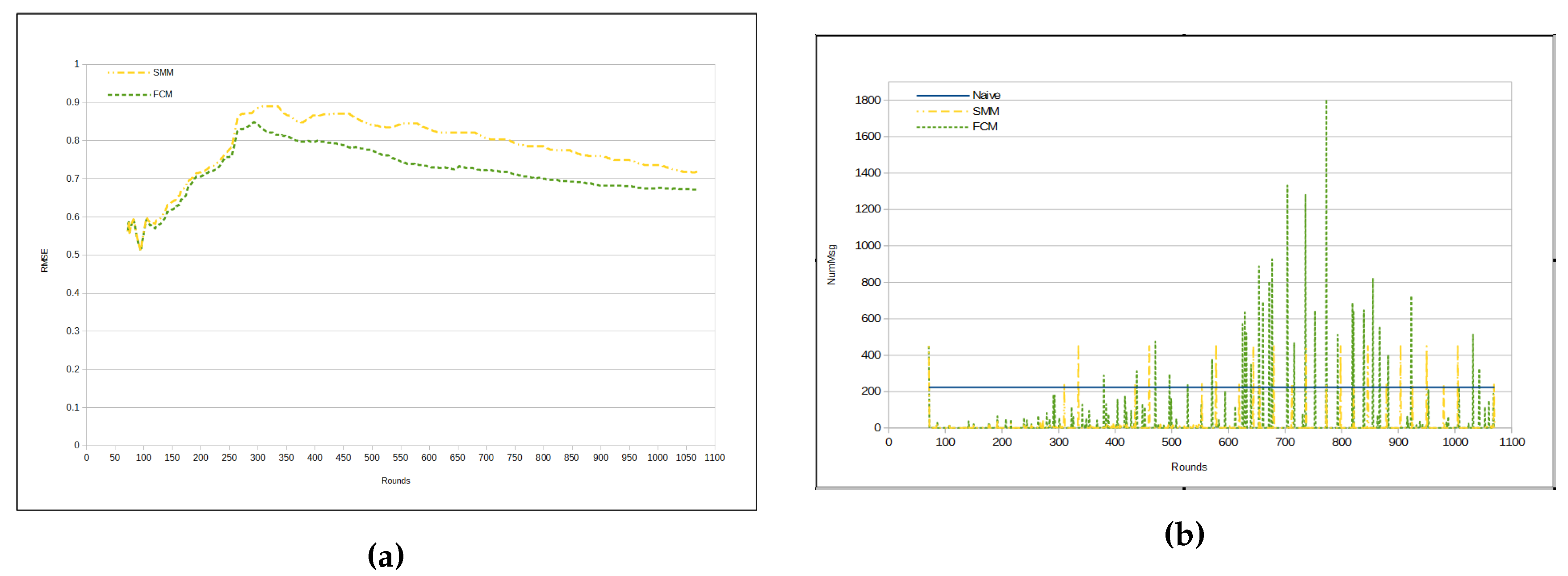
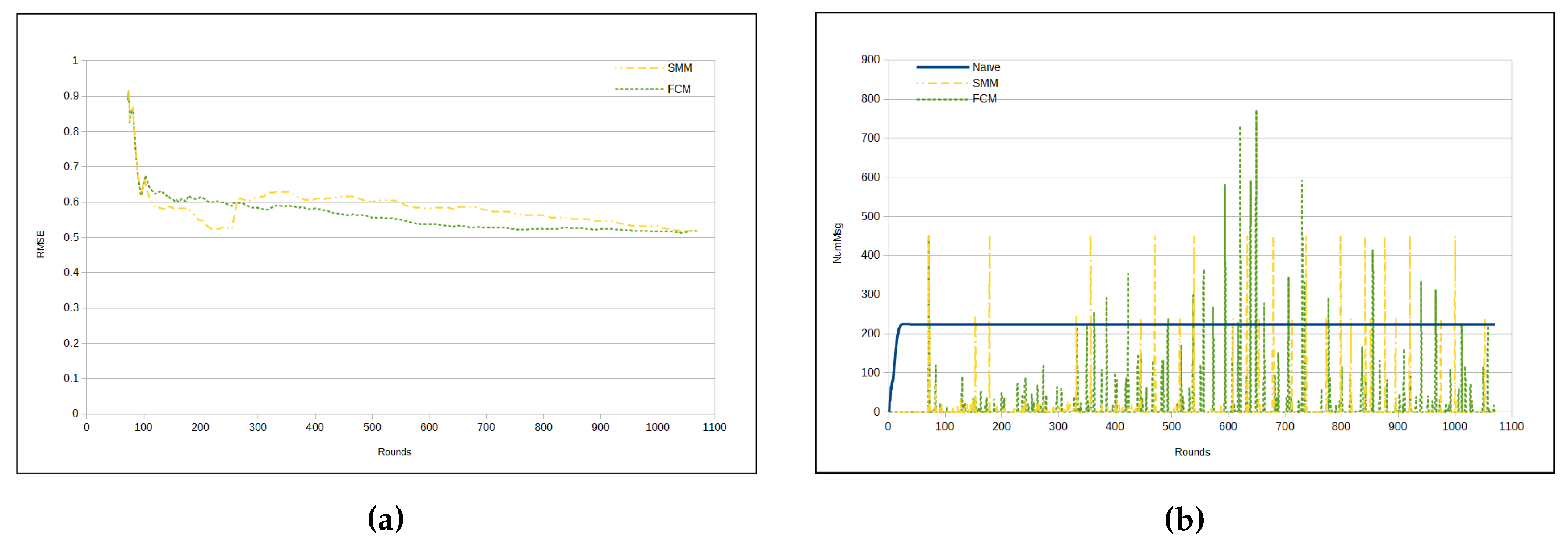
Figure 7a depicts evolution of RMSE per round. Observe that FCM and SMM RMSEs begin quite similarly. However, from a certain point in time on (approximately from round 110), they begin to present a different behavior, with an increase in the difference in round 260. From that point on, the FCM approach has a lower RMSE than the SMM approach (
Table 5).There is a peak for the both FCM and SMM lines, between rounds 300 and 350. The reason for that is the fact that the first cluster formation represents the initialization step for both approaches. Hence, both FCM and SMM accuracies are jeopardized at the beginning. Nevertheless, FCM and SMM approaches are able to automatically adjust the accuracy by reducing the RMSE through the use of
fractal clustering or
similarity measure, correspondingly. It is important to note that in the naive approach the RMSE is virtually 0 (zero). This is because all sensors send all sensed data to the sink.
Figure 7b presents the number of transmitted messages per round. In the naive approach, the number of messages is constant, since in each round all sensors send all sensed data to the sink. It is worth noting that there are some peaks in FCM and SMM curves, which represent periods in time, when clusters are being restructured (splitting or merging). Recall that these approaches (FCM and SMM) dynamically update the cluster configuration. Such a characteristic of the proposed approaches is responsible for the high standard deviation in
Table 6.
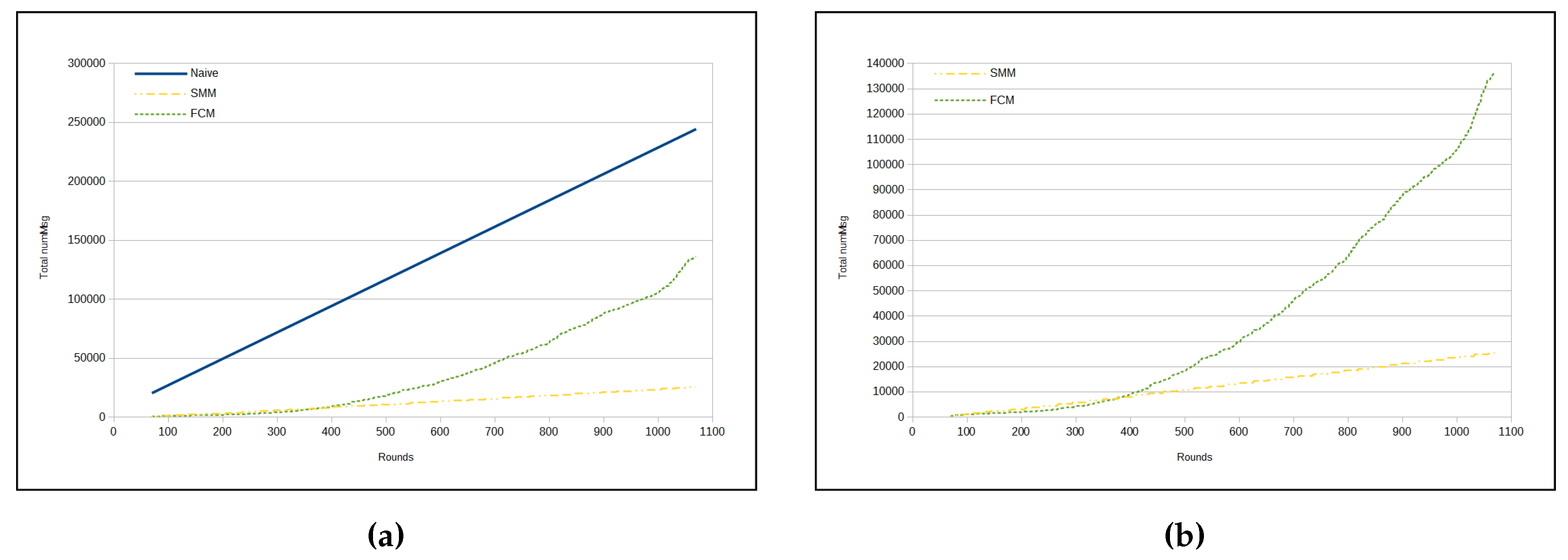
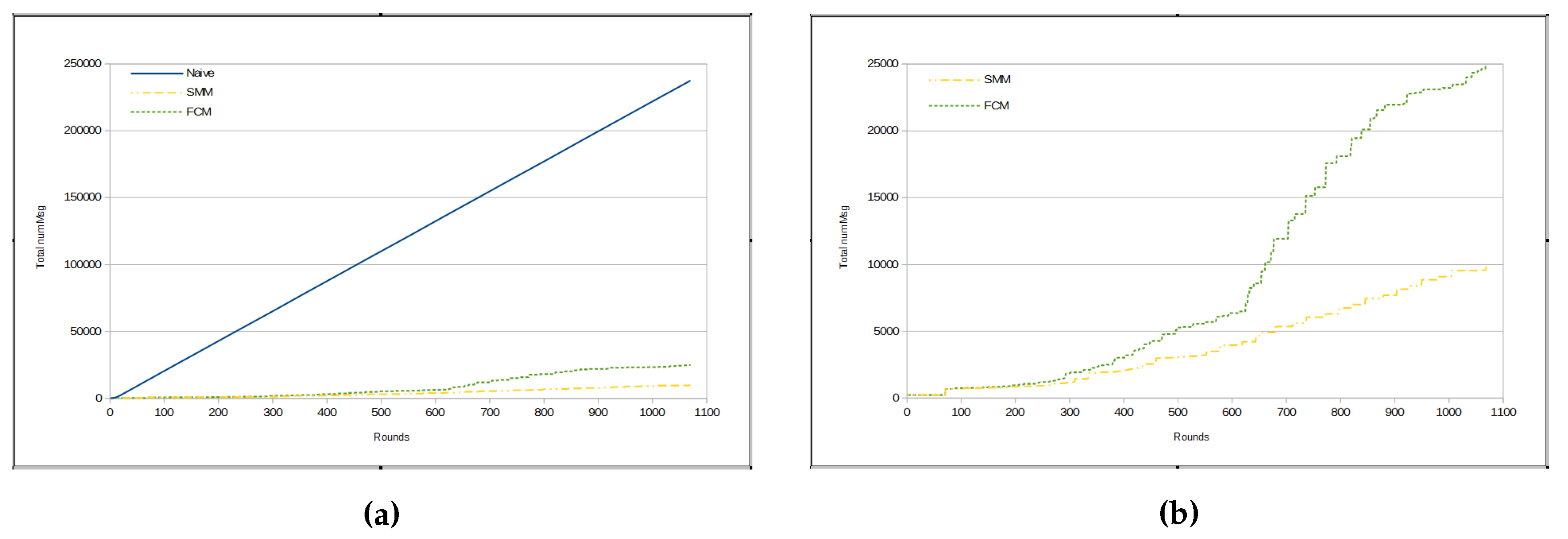
It can be inferred that the amount of messages sent per round in FCM approach is, mostly, bigger than in SMM. In fact, the total number of messages in the FCM approach has been shown to be much greater than the number of messages in SMM for
humidity measurements, as we can see in
Figure 8a,b.
Figure 8a presents a comparison among the total amount of messages from three approaches, namely naive, FCM and SMM. The total number of messages sent by sensors in naive approach is much greater than for the other two approaches, because in the previous method all sensors send all sensed data through messages immediately to the sink, whereas in other approaches there are some kinds of data suppression.
Next, we show the results obtained for the luminosity dimension, to compare a highly volatile (i.e., unpredictable) data type (such as luminosity), with a more predictable one (such as humidity).
As we can see in
Table 7, the RMSE values for
luminosity reveal that this physical phenomena has a very large variation, making it highly unpredictable. However, unlike the case of
humidity, in this situation the RMSE values for SMM approach were lower than for the FCM approach.
Despite the high number of messages compared to reading the
humidity, SMM approach again had the best results compared to FCM, in relation to the average number of sent messages per cycle for
luminosity data type (
Table 8).
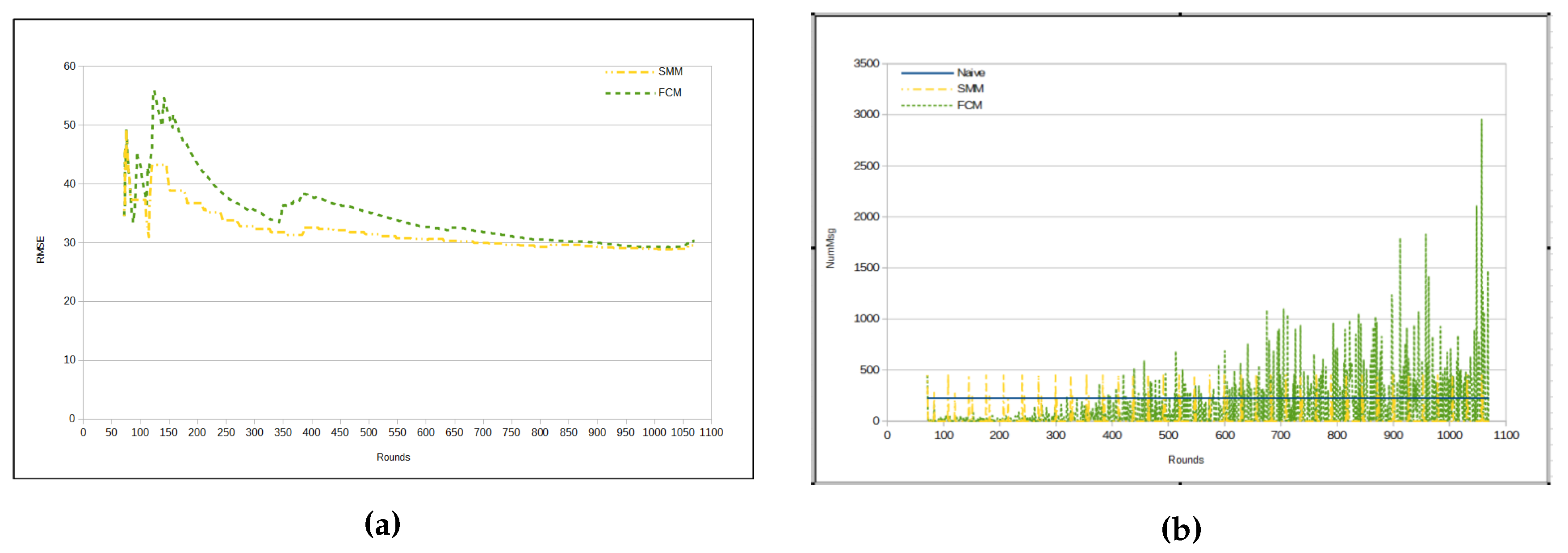
Figure 9a shows that when the RMSE of both approaches stabilizes, SMM has lower error than FCM approach. The number of messages per cycle starts smaller for FCM in comparison with SMM approach, whereas from about round 400 the FCM approach has significant peaks, reversing the situation presented until that point (
Figure 9b). This is due to the fact that the FCM approach deals with one sensor cluster reorganization per time, whereas the SMM approach makes a global merging process from time to time. As luminosity is highly unpredictable, a side effect is the shown high message exchange.
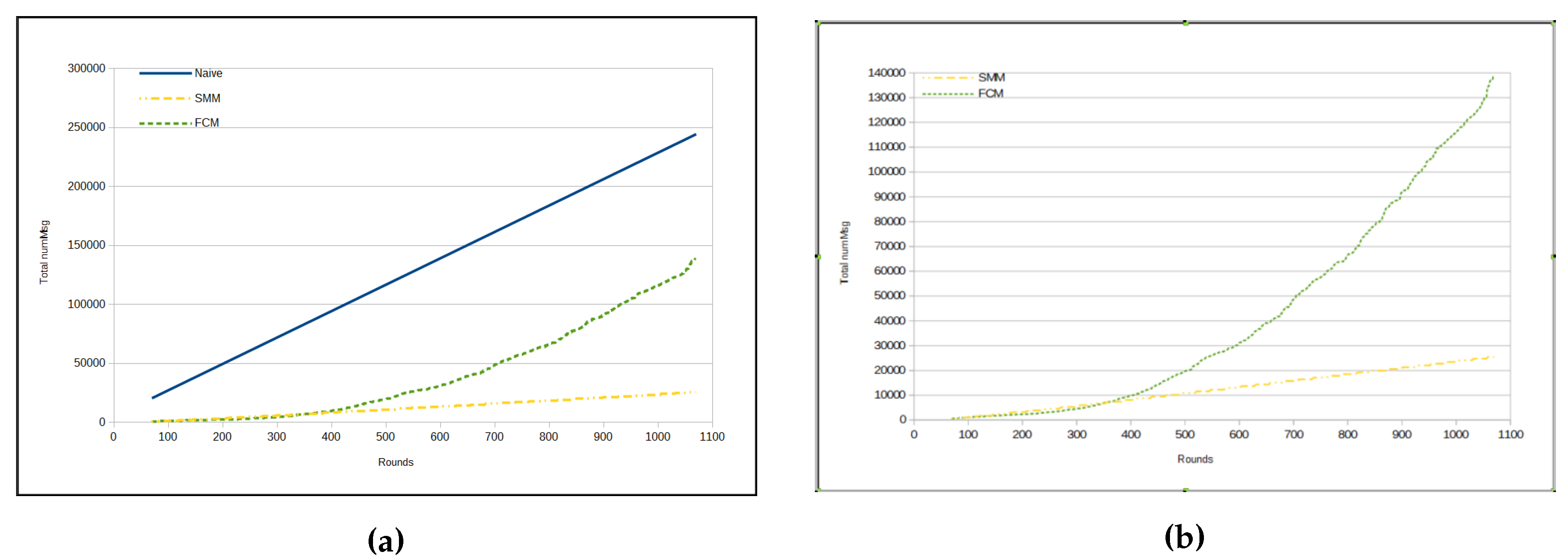
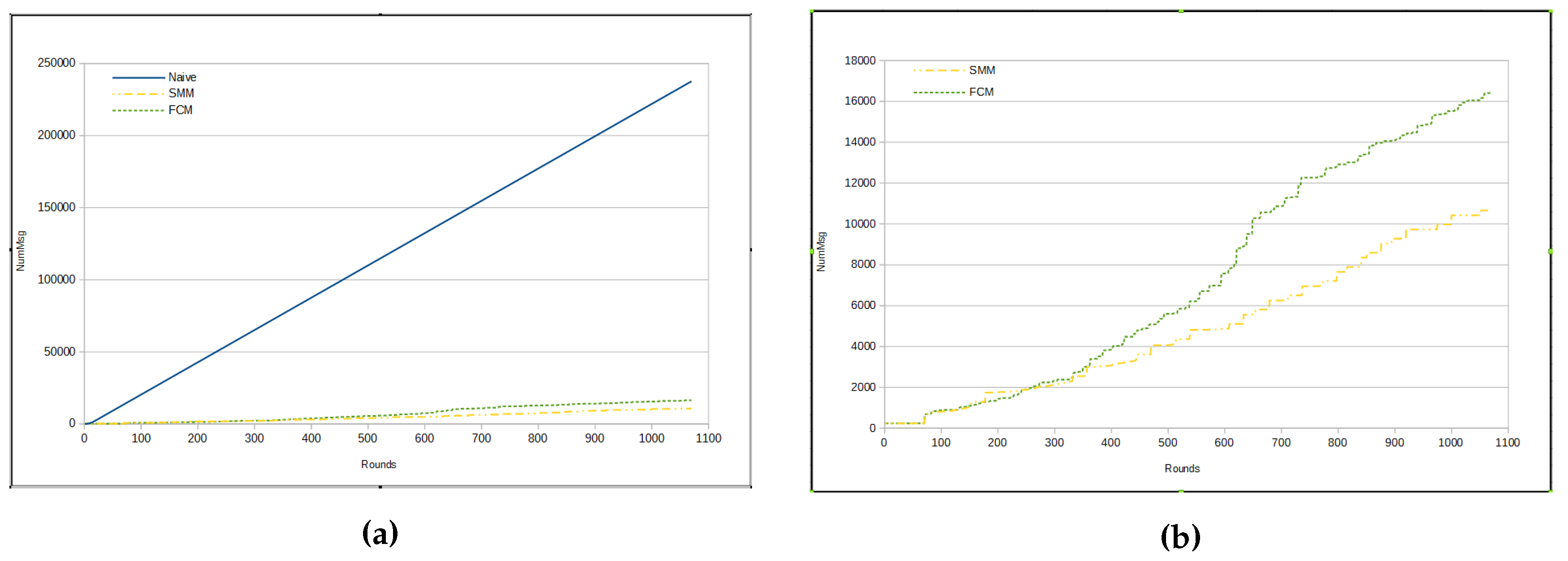
The total number of sent messages in both approaches is smaller than in the naive, mainly in the SMM approach. However, even for the FCM approach, the number of messages is approximately half that of the naive (see
Figure 10a). On the other hand,
Figure 10b shows that the SMM sends a smaller amount of messages than FCM from round 400 onwards.
Now, we compare the proposed approaches using two dimensions simultaneously, namely temperature and humidity.
Table 9 presents the results for RMSE, while using
temperature and
humidity as sensed data. As one can see, RMSE in this case is very similar to the cases with only one sensed data. As a matter of fact, RMSE is better in this case than it is with
humidity as unique sensed data. Comparing the two proposed approaches presented in
Table 9 and
Table 10, the relation between the approaches is maintained, in which the FCM approach presents a smaller RMSE than the SMM approach (
Figure 11a), and, in turn, the SMM injects a smaller number of messages in the WSN than the FCM approach (as in
Figure 11b,
Figure 12a,b).
Finally, we evaluate the proposed approaches using three dimensions at the same time: temperature, humidity and luminosity. The results show the ability of the proposed approaches to handle with multiple dimensions simultaneously.
In spite of the participation of
luminosity as data type, one can observe in
Table 11 that
temperature and
humidity together with
luminosity yield a RMSE reduction in comparison with
luminosity results (see
Table 7).
Comparing
Table 12 with
Table 8, we can see that the average number of messages per round in FCM approach for three data types (including
luminosity) is slightly larger than that for
luminosity only. However, the same parameter in SMM approach is virtually equal for the two cases. It is important to note that SMM approach presents an average number of messages much smaller than that of FCM approach in both situations.
Figure 13a presents a RMSE curve from the two approaches (namely SMM and FCM) applied to three data types with a behavior very similar to same approaches applied only to
luminosity, as one can see in
Figure 9a. However, it is important to note two major differences: (1) the magnitude of RMSE values, which in this situation is approximately half of the values of the previous case; and (2) the relative difference between the RMSE numbers for two approaches from round 800 onwards, which drops the difference virtually to zero, making the two approaches present very similar RMSEs.
With regard to the total number of messages sent, we can observe that there is a great similarity between the results made only with the
luminosity data type (
Figure 9b and
Figure 10a,b) and those made with the data types
temperature,
humidity and
luminosity (
Figure 13b,
Figure 14a,b).
Up to a point, for each graph showing the total number of messages for the two compared approaches (as in
Figure 8a,
Figure 10a,
Figure 12a and
Figure 14a), we made another graph which did not include the naive curve for the total number of messages (
Figure 8b,
Figure 10b,
Figure 12b and
Figure 14b), because it is too high due to the other two approaches.


 and
and 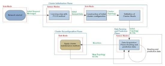


