
Optimization-Based Sensor Fusion of GNSS and IMU Using a Moving Horizon Approach


Abstract
:1. Introduction
2. Methods
2.1. Coordinate Frames
2.2. System Model
2.3. Sensor Models
2.3.1. Inertial Measurement Unit
2.3.2. GNSS Receiver
2.4. Optimization Problem
2.4.1. Measurement Residuals
2.4.2. Direct Collocation
2.4.3. Random Walk
2.5. MHE Estimator
3. Experimental Results
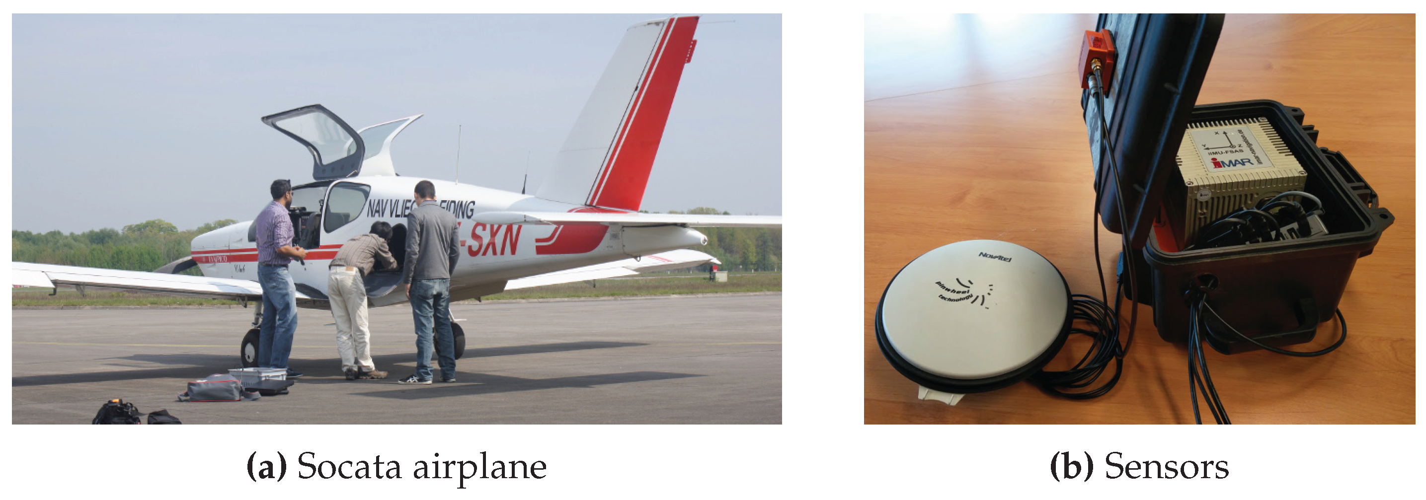
3.1. Dataset
3.2. Sensor Setup
3.3. Algorithm Configuration
3.4. Horizon Length Evaluation
4. Discussion
Acknowledgments
Author Contributions
Conflicts of Interest
References
- Verschueren, R.; Zanon, M.; Quirynen, R.; Diehl, M. Time-optimal race car driving using an online exact hessian based nonlinear MPC algorithm. In Proceedings of the European Control Conference (ECC), Aalborg, Denmark, 29 June–1 July 2016; pp. 141–147. [Google Scholar]
- Gros, S.; Zanon, M.; Vukov, M.; Diehl, M. Nonlinear MPC and MHE for Mechanical Multi-Body Systems with Application to Fast Tethered Airplanes. In Proceedings of the IFAC Conference on Nonlinear Model Predictive Control, Leeuwenhorst, The Netherlands, 23–27 August 2012; pp. 86–93. [Google Scholar]
- Chao, Z.; Ming, L.; Shaolei, Z.; Wenguang, Z. Collision-free UAV formation flight control based on nonlinear MPC. In Proceedings of the International Conference on Electronics, Communications and Control (ICECC), Ningbo, China, 9–11 September 2011; pp. 1951–1956. [Google Scholar]
- Russo, L.P.; Young, R.E. Moving-Horizon State Estimation Applied to an Industrial Polymerization Process. In Proceedings of the American Control Conference, San Diego, CA, USA, 2–4 June 1999; pp. 1129–1133. [Google Scholar]
- Hoffmann, G.; Gorinevsky, D.; Mah, R.; Tomlin, C.; Mitchell, J. Fault Tolerant Relative Navigation Using Inertial and Relative Sensors. In Proceedings of the AIAA Guidance, Navigation and Control Conference and Exhibit, Hilton Head, SC, USA, 20–23 August 2007. [Google Scholar]
- Quirynen, R.; Vukov, M.; Diehl, M. Auto Generation of Implicit Integrators for Embedded NMPC with Microsecond Sampling Times. In Proceedings of the IFAC Nonlinear Model Predictive Control Conference, Noordwijkerhout, The Nederlands, 23–27 August 2012; pp. 175–180. [Google Scholar]
- Frison, G.; Kufoalor, D.K.M.; Imsland, L.; Jorgensen, J.B. Efficient implementation of solvers for linear model predictive control on embedded devices. In Proceedings of the IEEE Conference on Control Applications (CCA), Juan Les Antibes, France, 8–10 October 2014; pp. 1954–1959. [Google Scholar]
- Hall, D.L.; Llinas, J. An introduction to multisensor data fusion. In Proceedings of the Circuits and Systems, Monterey, CA, USA, 31 May–3 June 1998. [Google Scholar]
- Sun, S.-L.; Deng, Z.-L. Multi-sensor optimal information fusion Kalman filter. Automatica 2004, 40, 1017–1023. [Google Scholar] [CrossRef]
- Mohamed, A.H.; Schwarz, K.P. Adaptive Kalman Filtering for INS/GPS. J. Geod. 1999, 73, 193–203. [Google Scholar] [CrossRef]
- Jwo, D.J.; Weng, T.P. An Adaptive Sensor Fusion Method with Applications in Integrated Navigation. In the Proceedings of the International Federation of Automatic Control, Seoul, Korea, 6–11 July 2008; pp. 9002–9007. [Google Scholar]
- Rao, C.V.; Rawlings, J.B.; Lee, J.H. Constrained Linear State Estimation—A Moving Horizon Approach. Automatica 2001, 37, 1619–1628. [Google Scholar] [CrossRef]
- Girrbach, F.; Hol, J.D.; Bellusci, G.; Diehl, M. Towards Robust Sensor Fusion for State Estimation in Airborne Applications Using GNSS and IMU. IFAC-PapersOnLine 2017, in press. [Google Scholar]
- Cox, D.B. Integration of GPS with Inertial Navigation Systems. Navigation 1978, 25, 236–245. [Google Scholar] [CrossRef]
- Crassidis, J. Sigma-point Kalman filtering for integrated GPS and inertial navigation. IEEE Trans. Aerosp. Electron. Syst. 2006, 42, 750–756. [Google Scholar] [CrossRef]
- Panzieri, S.; Pascucci, F.; Ulivi, G. An outdoor navigation system using GPS and inertial platform. IEEE/ASME Trans. Mech. 2002, 7, 134–142. [Google Scholar] [CrossRef]
- Honghui, Qi.; Moore, J. Direct Kalman filtering approach for GPS/INS integration. IEEE Trans. Aerosp. Electron. Syst. 2002, 38, 687–693. [Google Scholar] [CrossRef]
- Jones, E.S.; Soatto, S. Visual-inertial navigation, mapping and localization: A scalable real-time causal approach. Int. J. Robot. Res. 2011, 30, 407–430. [Google Scholar] [CrossRef]
- Crassidis, J.L.; Markley, F.L.; Cheng, Y. Survey of Nonlinear Attitude Estimation Methods. J. Guid. Control Dyn. 2007, 30, 12–28. [Google Scholar] [CrossRef]
- Gros, S.; Diehl, M. Attitude estimation based on inertial and position measurements. In Proceedings of the 51st IEEE Conference on Decision and Control (CDC), Maui, HI, USA, 10–13 December 2012; pp. 1758–1763. [Google Scholar]
- Haseltine, E.L.; Rawlings, J.B. Critical Evaluation of Extended Kalman Filtering and Moving-Horizon Estimation. Ind. Eng. Chem. Res. 2005, 44, 2451–2460. [Google Scholar] [CrossRef]
- Polóni, T.; Rohal-Ilkiv, B.; Arne Johansen, T. Moving Horizon Estimation for Integrated Navigation Filtering. IFAC-PapersOnLine 2015, 48, 519–526. [Google Scholar] [CrossRef]
- Gul, H.U.; Kai, D.Y. An Optimal Moving Horizon Estimation for Aerial Vehicular Navigation Application. In Proceedings of the IOP Conference Series: Materials Science and Engineering, Réunion Island, France, 10–13 October 2016. [Google Scholar]
- Vandersteen, J.; Diehl, M.; Aerts, C.; Swevers, J. Spacecraft Attitude Estimation and Sensor Calibration Using Moving Horizon Estimation. J. Guid. Control Dyn. 2013, 36, 734–742. [Google Scholar] [CrossRef]
- Rong Li, X.; Jilkov, V. Survey of maneuvering target tracking. Part I: Dynamic models. IEEE Trans. Aerosp. Electron. Syst. 2003, 39, 1333–1364. [Google Scholar] [CrossRef]
- Titterton, D.; Weston, J.L. Strapdown Inertial Navigation Technology; AIAA: Reston, VA, USA, 2004; p. 558. [Google Scholar]
- El-Sheimy, N.; Hou, H.; Niu, X. Analysis and Modeling of Inertial Sensors Using Allan Variance. IEEE Trans. Instrum. Meas. 2008, 57, 140–149. [Google Scholar] [CrossRef]
- Savage, P.G. Strapdown Inertial Navigation Integration Algorithm Design Part 1: Attitude Algorithms. J. Guid. Control Dyn. 1998, 21, 19–28. [Google Scholar] [CrossRef]
- Kaplan, E.D.; Hegarty, C.J. Understanding GPS : Principles and Applications; Artech House: Norwood, MA, USA, 2006; p. 703. [Google Scholar]
- Von Stryk, O. Numerical Solution of Optimal Control Problems by Direct Collocation. In Optimal Control; Birkhäuser Basel: Basel, Switzerland, 1993; pp. 129–143. [Google Scholar]
- Bock, H.G.; Diehl, M.M.; Leineweber, D.B.; Schlöder, J.P. A Direct Multiple Shooting Method for Real-Time Optimization of Nonlinear DAE Processes. In Nonlinear Model Predictive Control; Birkhäuser Basel: Basel, Switzerland, 2000; pp. 245–267. [Google Scholar]
- Butcher, J.C. Integration Processes Based on Radau Quadrature Formulas. Math. Comput. 1964, 18, 233. [Google Scholar] [CrossRef]
- Wang, S.; Chen, L.; Gu, D.; Hu, H. An Optimization Based Moving Horizon Estimation with Application to Localization of Autonomous Underwater Vehicles. Robot. Auton. Syst. 2014, 62, 1581–1596. [Google Scholar] [CrossRef]
- Xsens Technologies B.V. Xsens MTi-G-710 Motion Tracker. 2017. Available online: https://www.xsens.com/products/mti-g-700/ (accessed on 12 May 2017).
- iMAR Navigation GmbH. iIMU-FSAS: IMU with Odometer Interface and Integrated Power Regulation. Available online: http://www.imar-navigation.de/downloads/IMU_FSAS.pdf (accessed on 12 May 2017).
- Vydhyanathan, A.; Bellusci, G.; Luinge, H.; Slycke, P. The Next Generation Xsens Motion Trackers for Industrial Applications. 2015. Available online: https://www.xsens.com/download/pdf/documentation/mti/mti_white_paper.pdf (accessed on 12 May 2017).
- Diehl, M.; Bock, H.G.; Schlöder, J.P. A Real-Time Iteration Scheme for Nonlinear Optimization in Optimal Feedback Control. SIAM J. Control Optim. 2005, 43, 1714–1736. [Google Scholar] [CrossRef]


 ).
).
).
).

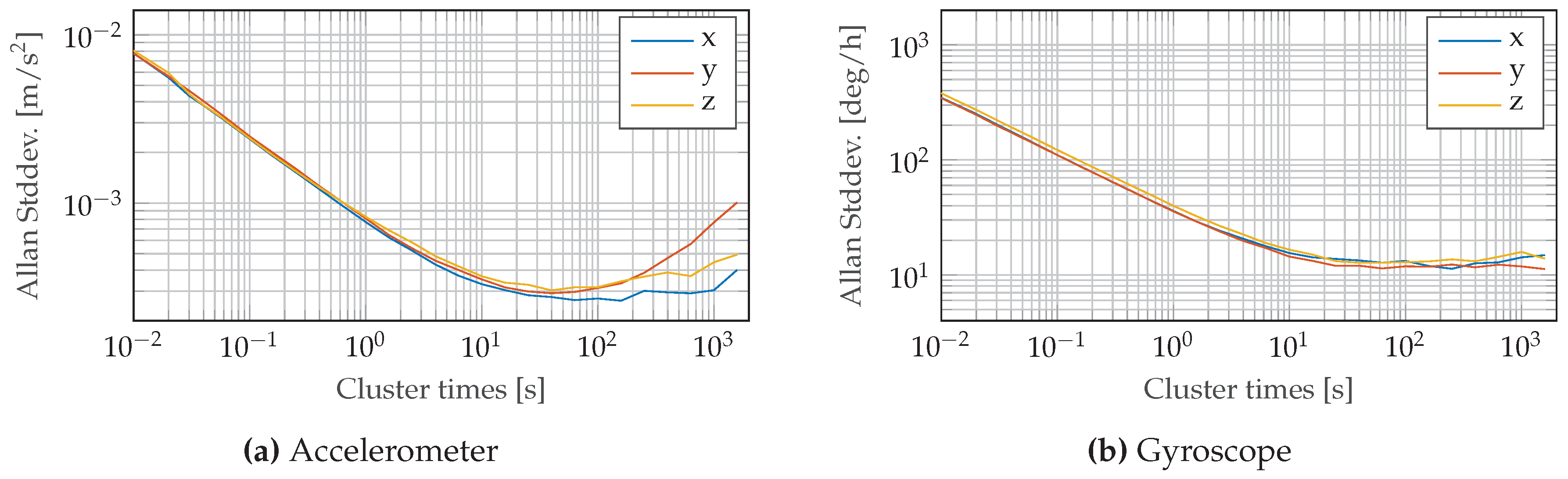
 , y
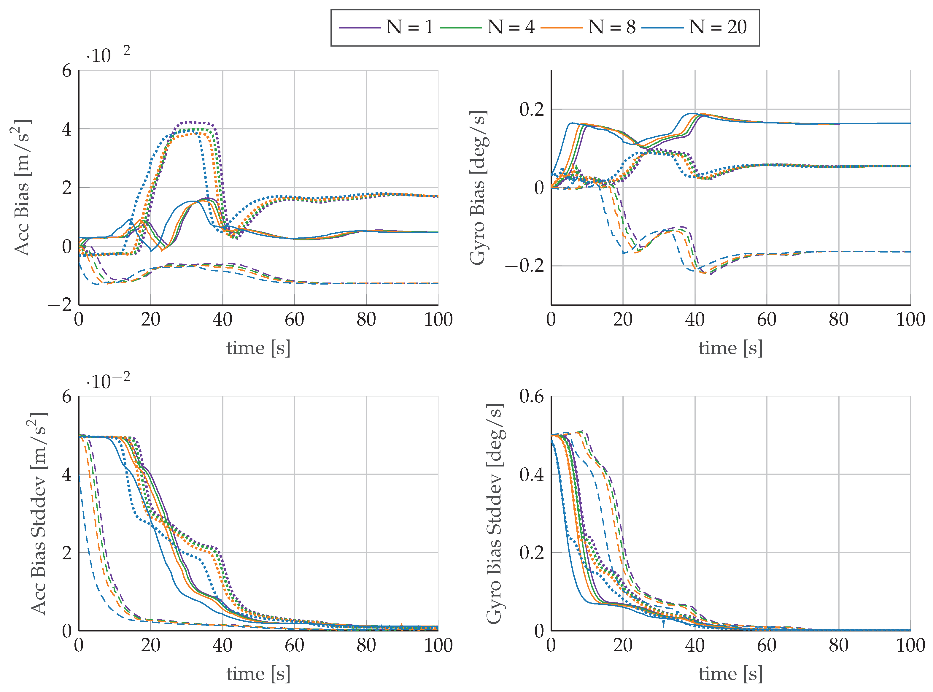
, y  , z----) of accelerometer and gyroscope and their corresponding standard deviations for different horizons N.
, y , z----) of accelerometer and gyroscope and their corresponding standard deviations for different horizons N.
, z----) of accelerometer and gyroscope and their corresponding standard deviations for different horizons N.
, y , z----) of accelerometer and gyroscope and their corresponding standard deviations for different horizons N.
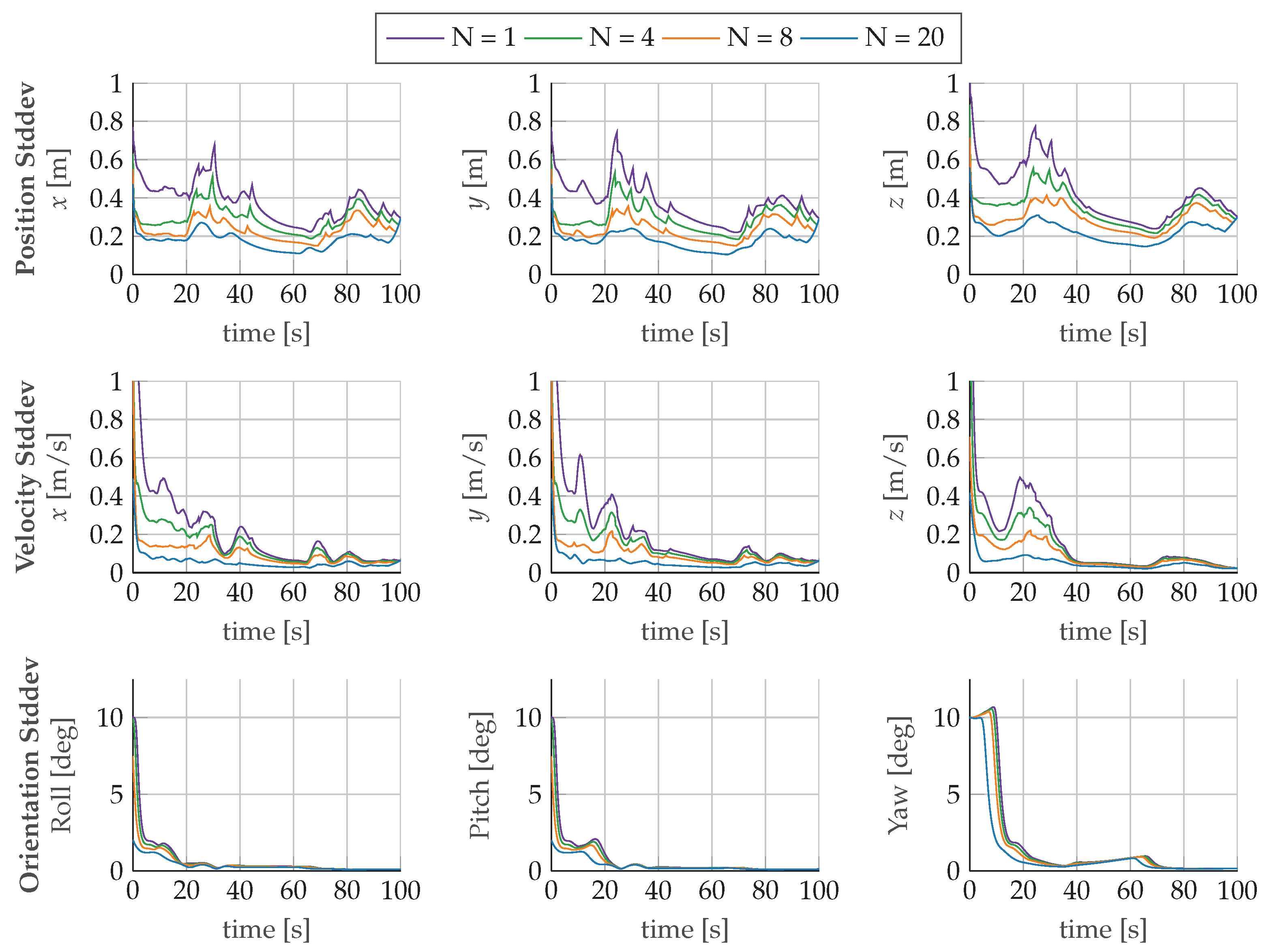
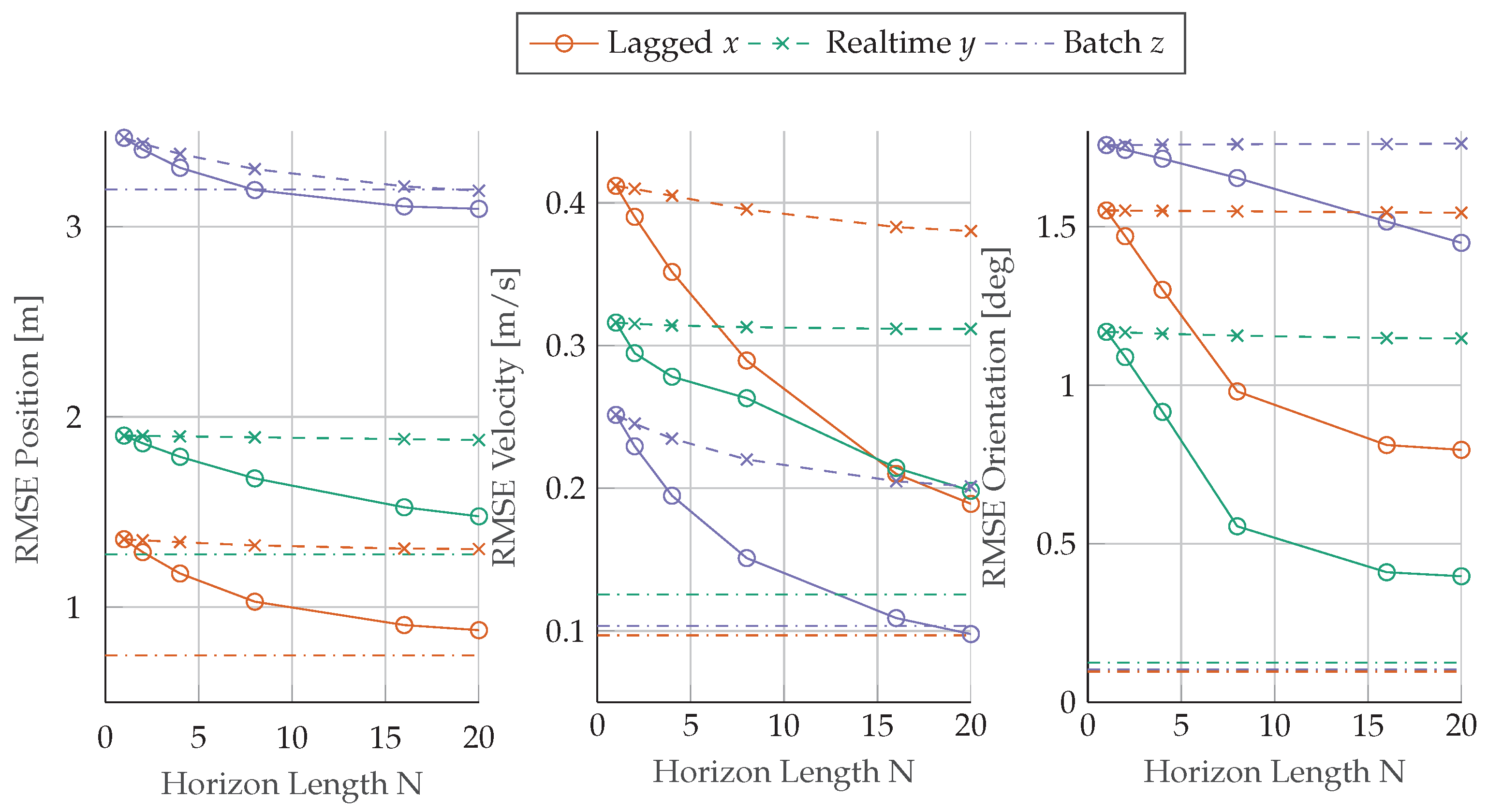
 ) and lagged (−×−) mhe estimators over an increasing horizon length N compared to the batch estimation results (−·−·−).
) and lagged (−×−) mhe estimators over an increasing horizon length N compared to the batch estimation results (−·−·−).
) and lagged (−×−) mhe estimators over an increasing horizon length N compared to the batch estimation results (−·−·−).


| Estimation | Reference | ||
|---|---|---|---|
| IMU | MTi-G-700 | iMAR-FSAS | |
| Gyro Technology | MEMS | FOG | |
| Gyro Rate Bias Repeatability | |||
| Gyro Rate Bias Stability | 10 | ||
| Angular Random Walk | |||
| Accelerometer Technology | MEMS | Servo | |
| Accelerometer Bias Repeatability | |||
| Accelerometer Bias Stability | [g] | 40 | |
| Accelerometer Random Walk | [g] | 80 | |
| GNSS | MTi-G-700 | FlexPak-V2-RT2 | |
| Constellation | GPS | GPS + GLONASS | |
| Bands | + (DGPS) | ||
| Accuracy | 2–4 | ||
| max. Rate | 4 | 40 |
| Parameter | Unit | Value | Standard Deviation |
|---|---|---|---|
| Position | 10 | ||
| Velocity | 5 | ||
| Orientation | 8 | ||
| Accelerometer Bias | 0 | ||
| Gyroscope Bias | 0 |
© 2017 by the authors. Licensee MDPI, Basel, Switzerland. This article is an open access article distributed under the terms and conditions of the Creative Commons Attribution (CC BY) license (http://creativecommons.org/licenses/by/4.0/).
Share and Cite
Girrbach, F.; Hol, J.D.; Bellusci, G.; Diehl, M. Optimization-Based Sensor Fusion of GNSS and IMU Using a Moving Horizon Approach. Sensors 2017, 17, 1159. https://doi.org/10.3390/s17051159
Girrbach F, Hol JD, Bellusci G, Diehl M. Optimization-Based Sensor Fusion of GNSS and IMU Using a Moving Horizon Approach. Sensors. 2017; 17(5):1159. https://doi.org/10.3390/s17051159
Chicago/Turabian StyleGirrbach, Fabian, Jeroen D. Hol, Giovanni Bellusci, and Moritz Diehl. 2017. "Optimization-Based Sensor Fusion of GNSS and IMU Using a Moving Horizon Approach" Sensors 17, no. 5: 1159. https://doi.org/10.3390/s17051159
APA StyleGirrbach, F., Hol, J. D., Bellusci, G., & Diehl, M. (2017). Optimization-Based Sensor Fusion of GNSS and IMU Using a Moving Horizon Approach. Sensors, 17(5), 1159. https://doi.org/10.3390/s17051159