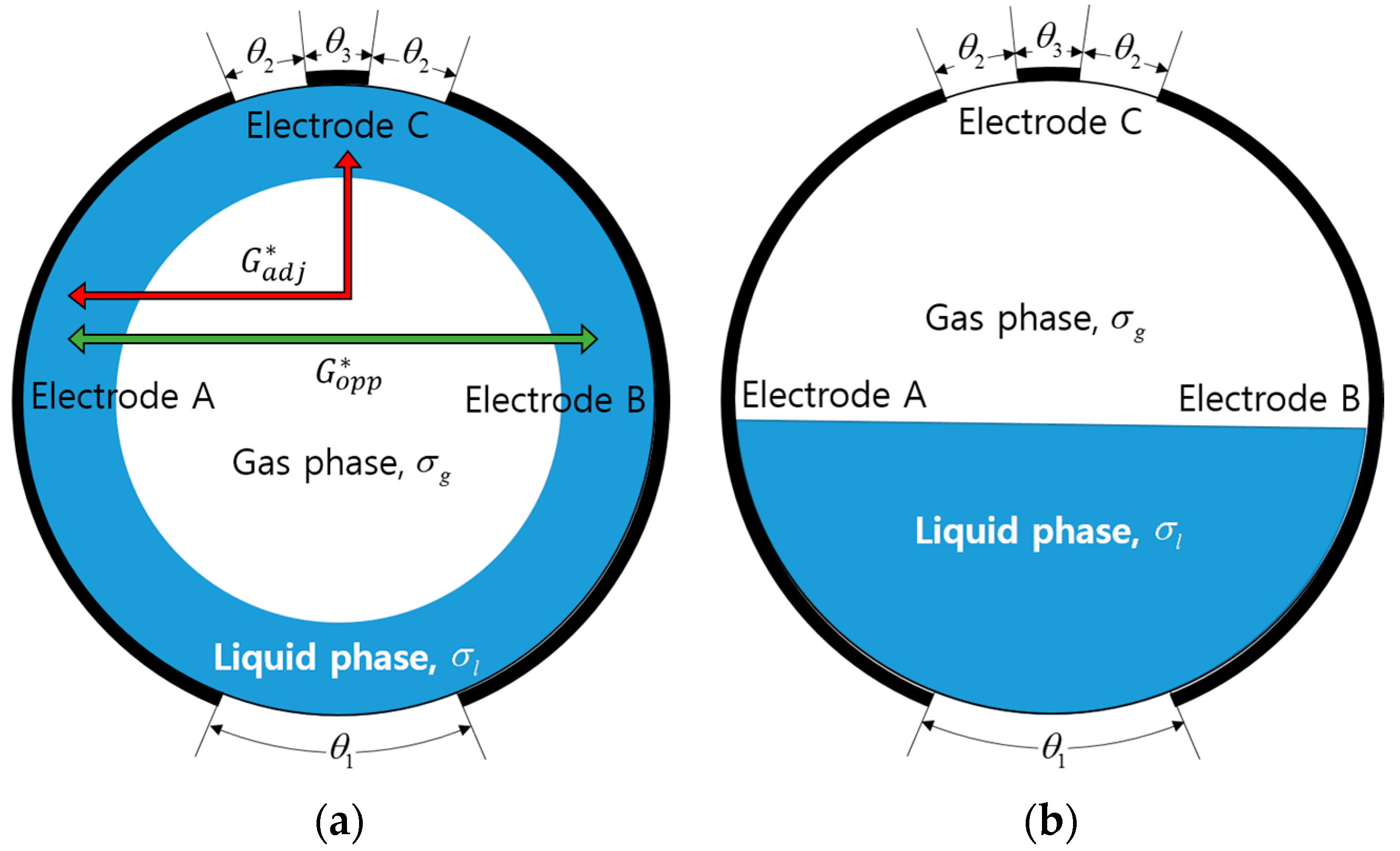
Figure 1.
Configuration of electrodes in the proposed conductance sensor and typical flow structures considered: (a) Annular flow condition; (b) Stratified flow condition.
Figure 1.
Configuration of electrodes in the proposed conductance sensor and typical flow structures considered: (a) Annular flow condition; (b) Stratified flow condition.
Figure 2.
An improved dual conductance sensor system for measurement of the structure velocity.
Figure 2.
An improved dual conductance sensor system for measurement of the structure velocity.
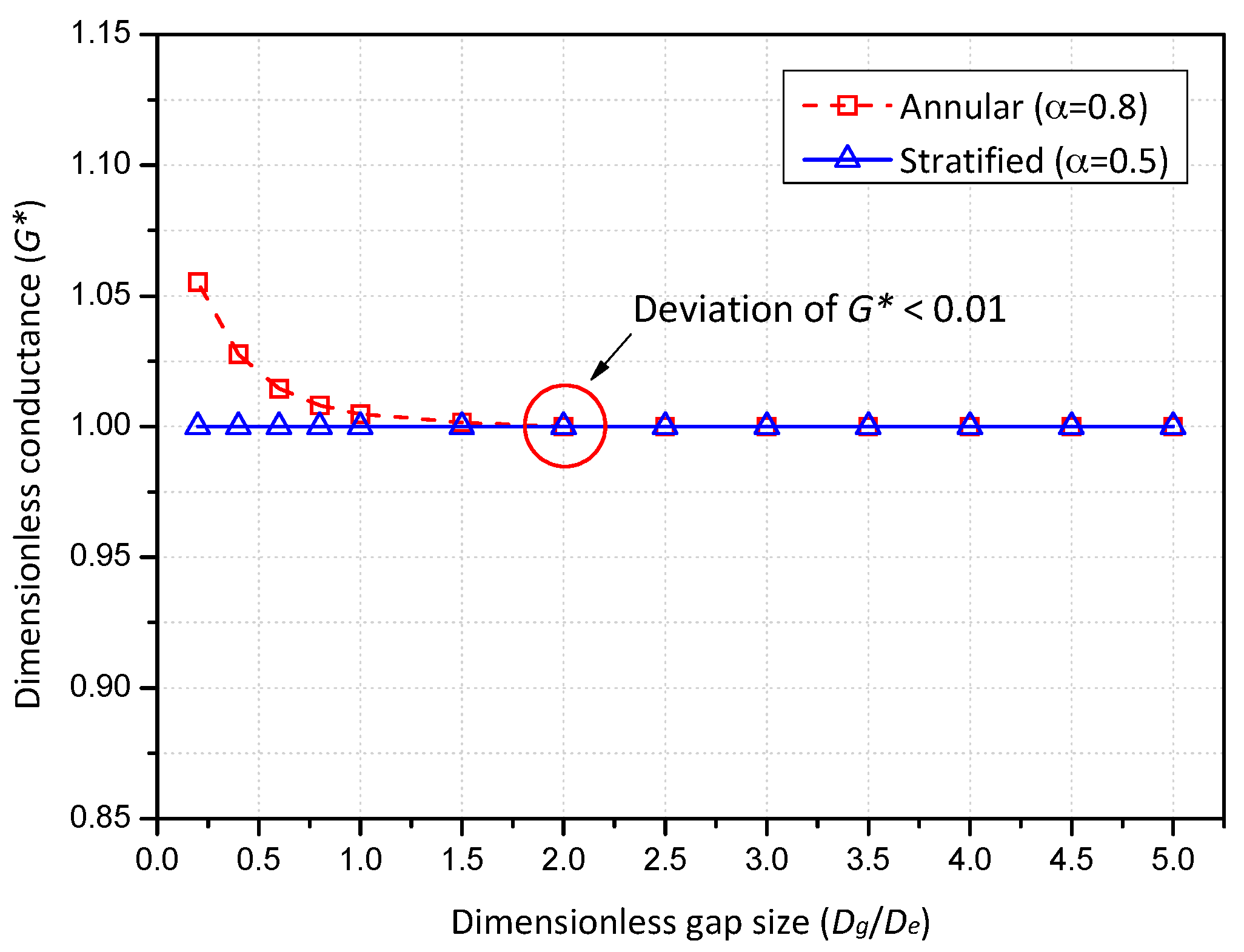
Figure 3.
Variation of the calculated conductance according to the spacing between layers.
Figure 3.
Variation of the calculated conductance according to the spacing between layers.
Figure 4.
Predicted and measured dimensionless conductance as a function of the void fraction: (a) Annular flow; (b) Stratified flow.
Figure 4.
Predicted and measured dimensionless conductance as a function of the void fraction: (a) Annular flow; (b) Stratified flow.
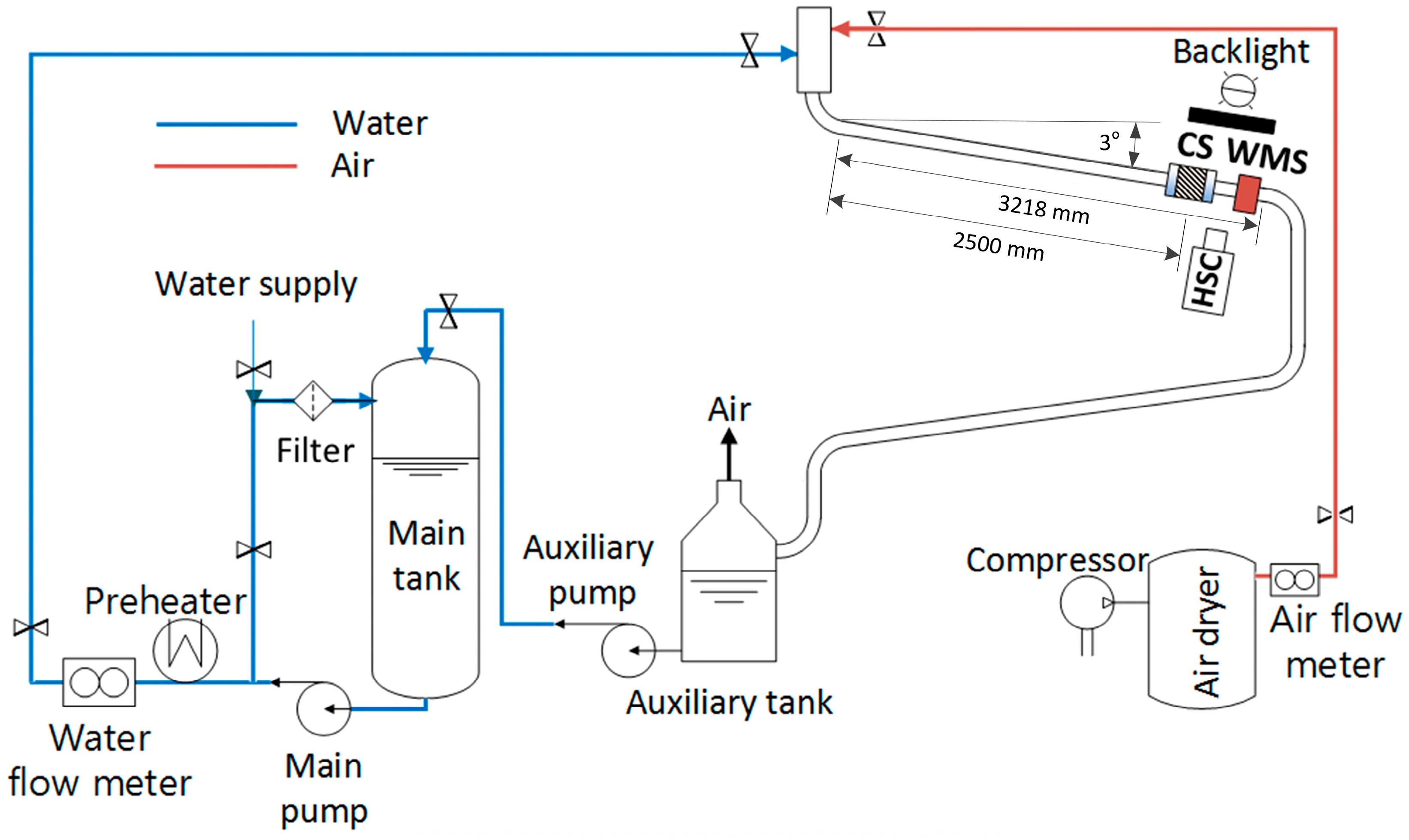
Figure 5.
Schematic diagram of the air-water two-phase flow loop.
Figure 5.
Schematic diagram of the air-water two-phase flow loop.
Figure 6.
Schematic diagram of the air-water two-phase flow loop.
Figure 6.
Schematic diagram of the air-water two-phase flow loop.
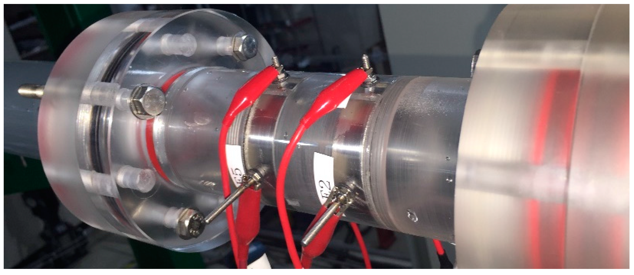
Figure 7.
Measurement system for the conductance sensor.
Figure 7.
Measurement system for the conductance sensor.
Figure 8.
Investigated flow conditions marked on the flow regime map by Taitel and Dukler [
23] (the colored marks indicate the selected runs to be discussed in
Section 4.2. Measurement Results. The reds are to investigate the effect of the liquid velocity at a fixed gas velocity, whereas the blues indicates tests performed at a fixed liquid velocity with varying the gas velocity. The dash-line box encloses the testable ranges in the JNU two-phase flow loop).
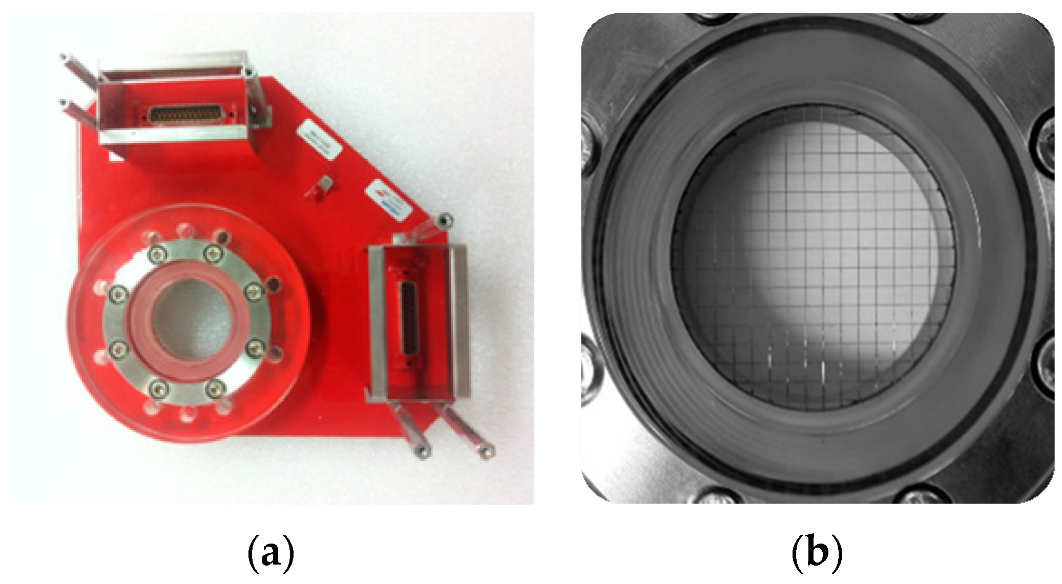
Figure 9.
Wire-mesh sensor manufactured by HZDR Inc. (Dresden, Germany) for validation of the measured void fraction. (a) Photograph of the wire-mesh sensor used in this study. (b) Transmitter and receiver electrodes mesh of the wire-mesh sensor.
Figure 9.
Wire-mesh sensor manufactured by HZDR Inc. (Dresden, Germany) for validation of the measured void fraction. (a) Photograph of the wire-mesh sensor used in this study. (b) Transmitter and receiver electrodes mesh of the wire-mesh sensor.
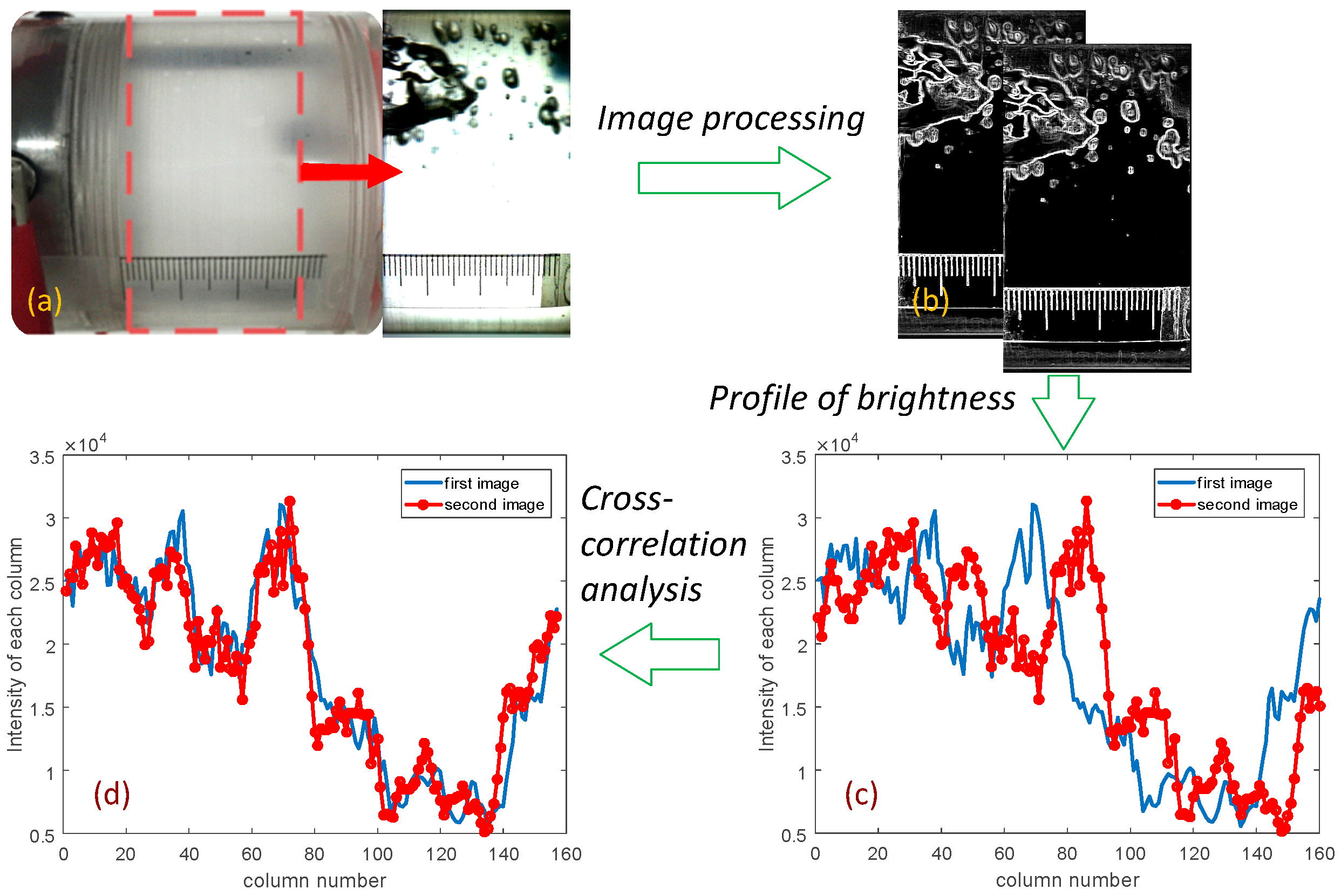
Figure 10.
Cross-correlation method using the visualized images for verification of the measured structure velocity. (a) Visualized image recorded by the high-speed camera. (b) Phase edge detection applied to two images captured with a known time interval. (c) Distributions of the brightness integrated by column. (d) Shift in distance determined by the cross-correlation analysis for the best match of the brightness distributions.
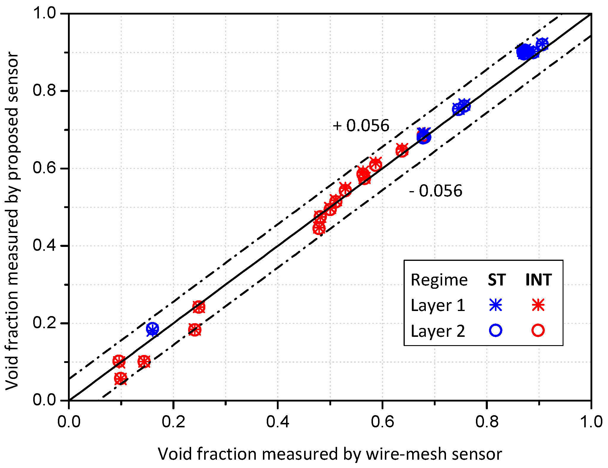
Figure 11.
Comparison between the time-averaged void fractions measured by the proposed sensor and the wire-mesh sensor (note: ST and INT stand for the stratified and intermittent flow regimes, respectively).
Figure 11.
Comparison between the time-averaged void fractions measured by the proposed sensor and the wire-mesh sensor (note: ST and INT stand for the stratified and intermittent flow regimes, respectively).
Figure 12.
The results of the flow pattern classification and the corresponding time series of the void fraction with varying the liquid superficial velocity (Note: The right Y-axis of the lower graphs indicates the dimensionless conductance.) (a) Case 1: jl = 0.1 m/s, jg = 10 m/s, jsv = 1.18 m/s. (b) Case 2: jl = 0.5 m/s, jg = 10 m/s, jsv = 1.96 m/s. (c) Case 3: jl = 1.0 m/s, jg = 10 m/s, jsv = 2.77 m/s. (d) Case 4: jl = 2.0 m/s, jg = 10 m/s, jsv = 4.27 m/s. (e) Case 5: jl = 3.0 m/s, jg = 10 m/s, jsv = 6.38 m/s.
Figure 13.
The results of the flow pattern classification and the corresponding time series of the void fraction with varying the gas superficial velocity (Note: The right Y-axis of the lower graphs indicates the dimensionless conductance). (a) Case 6: jl = 2.0 m/s, jg = 0.1 m/s, jsv = 2.04 m/s. (b) Case 7: jl = 2.0 m/s, jg = 0.5 m/s, jsv = 2.29 m/s. (c) Case 8: jl = 2.0 m/s, jg = 1.0 m/s, jsv = 2.49 m/s. (d) Case 9: jl = 2.0 m/s, jg = 5.0 m/s, jsv = 4.05 m/s. (e) Case 10: jl = 2.0 m/s, jg = 12 m/s, jsv = 4.91 m/s.
Figure 14.
The relationship between the structure velocity and the mixture velocity: (a) jl = 0.1~0.8 m/s; (b) jl = 1.0~3.0 m/s.
Figure 14.
The relationship between the structure velocity and the mixture velocity: (a) jl = 0.1~0.8 m/s; (b) jl = 1.0~3.0 m/s.
Table 1.
Electrical properties and sensor dimensions for the numerical calculation.
Table 1.
Electrical properties and sensor dimensions for the numerical calculation.
| Variables | Value |
|---|
| Conductivity (S/m) | Water | 0.005 |
| Air | 0 |
| Electrode | 1.0 × 10⁶ |
| Gap | 0 |
| Applied voltage (V) | 5 |
| Signal frequency (kHz) | 10 |
| Inner diameter of the sensor (mm) | 45 |
| Width of electrodes (De, mm) | 15 |
| Dimensionless gap size (Dg/De) | 0.25~5 |
Table 2.
Details of the optimized sensor configurations.
Table 2.
Details of the optimized sensor configurations.
| Variables | Value |
|---|
| Circumferential size (rad) | Electrode A & B | 2.54 |
| Electrode C | 0.30 |
| Inner diameter of the sensor (mm) | 45 |
| Width of electrodes (De, mm) | 15 |
| Thickness of electrodes (mm) | 2 (concave) |
| Spacing between layers (mm) | 30 |
Table 3.
Criteria for flow pattern classification.
Table 3.
Criteria for flow pattern classification.
| | Flow Regime |
|---|
| <0.01 | - | Stratified flow |
| ≥0.01 | < | Annular flow |
| ≥ | Intermittent flow |
Table 4.
Specifications of measurement instruments used for experiments.
Table 4.
Specifications of measurement instruments used for experiments.
| Instruments | Accuracy | Signal Range | Time Definition |
|---|
| Agilent 4284A LCR meter | 0.05~0.5% | Up to 20 V with 1 MHz | N/A |
| NI PXI-2536 | N/A | Up to ±12 V and 100 mA | 5 × 10⁴ cross-points/s |
| NI PXIe-6368 | 3 mV for ±10 V range | Up to ±10 V | 2 × 10⁶ samples/channel |
Table 5.
Test matrix for air-water two-phase flow experiments in the inclined loop.
Table 5.
Test matrix for air-water two-phase flow experiments in the inclined loop.
| Run | jl (m/s) | jg (m/s) | Flow Pattern “by Map” |
|---|
| 1~5 | 0.1 | 0.1, 0.5, 1, 5, 10, 12 | Stratified flow |
| 6 | 0.3 | 18 | Annular low |
| 7~11 | 0.5 | 0.1, 0.5, 1, 5, 10, 12 | Stratified flow |
| 12~16 | 1 | Intermittent flow |
| 17~21 | 2 | Intermittent flow |
| 22~25 | 3 | 0.1, 0.5, 1, 10 | Intermittent flow |
Table 6.
Validation results of the structure velocities measured by the conductance sensor.
Table 6.
Validation results of the structure velocities measured by the conductance sensor.
| Case | jl (m/s) | jg (m/s) | jsv (m/s) | Deviation |
|---|
| Conductance Sensor | High Speed Camera |
|---|
| A | 1.8 | 5.0 | 3.58 | 3.60 | −0.56% |
| B | 2.2 | 0.3 | 2.65 | 2.62 | 1.2% |
| C | 2.5 | 2.0 | 3.94 | 3.88 | 1.6% |
| D | 3.0 | 0.5 | 3.19 | 3.16 | 0.95% |
| E | 3.0 | 1.0 | 3.66 | 3.66 | 0% |


