1. Introduction
Nowadays, urban rail transit systems are vastly utilized in modern cities of the world due to their high capability and capacity in transferring passengers, air pollution reduction, traffic reduction in crowded cities, optimal utilization of energy resources, and their fast speed [
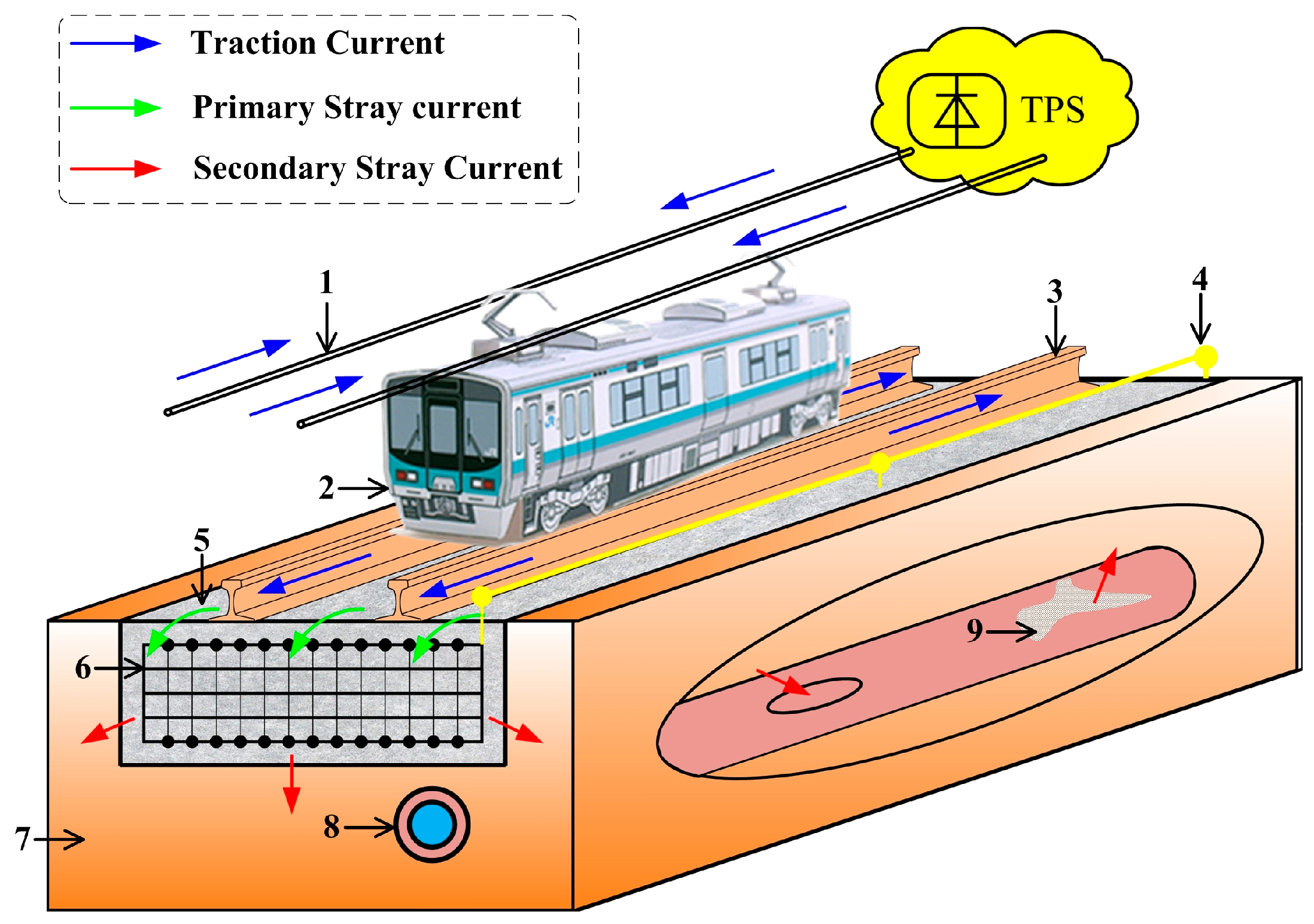
1]. For the purpose of reducing the construction cost and the maintenance cost, running rails usually act as the return path of traction current in the urban rail transit system. The running rails have limited conductivity and are not completely insulated over the ground, so a part of the traction current will flow into the earth without returning to the traction substation (TPS). This kind of current underground is called ‘stray current’. The stray current can be divided into two parts. The current leaving running rails will flow into the stray current control mat, which is called the primary stray current. Most of the primary stray current will return to the TPS again, the remaining current will flow into the soil beneath, which is called the secondary stray current [
2]. If the secondary stray current flows into the buried pipe, the corrosion of buried pipe will occur from each point that current transfers from the buried pipe to the electrolyte [
3]. The stray current formation mechanism is shown in
Figure 1. It is noted that there have been a lot of severe cases concerning secondary stray current corrosion. For example, after starting the operation of the Guangzhou metro line 1 in 1999, the maintenance of the mid-pressure gas network built by Guangzhou Gas Group Co. Ltd. has gone up substantially. The maintenance cases numbered about 13 in 1998 while they were about 248 in 2011, which have been proven to be closely related to the secondary stray current corrosion from the Guangzhou metro line 1. According to our test results in Guangzhou metro at a constant temperature (about 20 °C), the maximum value of the secondary stray current is about 28.94 A while its minimum value is about 14.07 A. Thus, there is a secondary stray current measurement requirement to minimize its impact on the buried pipe.
The optical fiber current sensor (OFCS) has many advantages compared with the traditional electric sensors, including inherent safety, passive type, and anti-corrosion. It has attracted wide attention in the past three decades. For example, an OFCS has been proposed based on the Fabry-Perot interferometer using a fiber Bragg grating demodulation [
4]; an OFCS has been reported based on a long-period fiber grating with a permanent magnet [
5]; and an OFCS has been designed based on microfiber and chrome-nickel wire [
6]. Moreover, the most widely used OFCS mechanism by far, the Faraday effect, which has been explored in many configurations [
7,
8,
9,
10]. In this case, the light propagating in a sensing fiber experiences a rotation in the angle of polarization in the presence of an external magnetic field. According to the Faraday effect, we have proposed the stray current sensor [
11,
12], which has been successfully applied for the secondary stray current measurement in Guangzhou metro. The main problem in the practical application is that the measurement accuracy of the stray current sensor is greatly limited by the temperature-induced linear birefringence (TILB). As far as we know, there are four effective methods that have improved elimination of the TILB. The first method applies the thermally annealed fiber as the sensing fiber [
8]. However, the thermally annealed fiber is found to be easily damaged. The second method applies the twisted fiber as the sensing fiber [
13]. However, the effect of this method is gradually decreased over time due to the release of the shearing stress produced by the torsion operation. The third method applies highly spun birefringence fiber as the sensing fiber [
14]. However, the Verdet constant of this fiber is difficult to be evenly distributed. Moreover, this fiber needs to be improved in some ways, such as the high polarization mode dispersion and the high cost of fabrication. The last method applies the Faraday mirror to eliminate the TILB. However, this method is effective only when the Faraday rotation angle (single pass) is 45 deg [
15]. In fact, this Faraday rotation angle is very sensitive to the external magnetic field [
16].
In this paper, an elimination method of the TILB in the stray current sensor is proposed. This method follows the idea that the sensing fiber in the sensor head is designed as the CSF based on geometric rotation effect, which produces a large amount of circular birefringence to suppress the TILB. The structure of this paper is arranged as follows: Firstly, the configuration and principle of the stray current sensor are demonstrated. Then, the differential equations that indicate the polarization evolution of the CSF element are derived. The output error model is built based on the Jones matrix calculus. On these bases, an accurate search method is proposed to obtain the key parameters of the CSF, including the length of the cylindrical silica rod and the number of the curve spirals. Finally, temperature experiments are conducted to verify the feasibility of this elimination method.
3. Output Error Mode of Stray Current Sensor
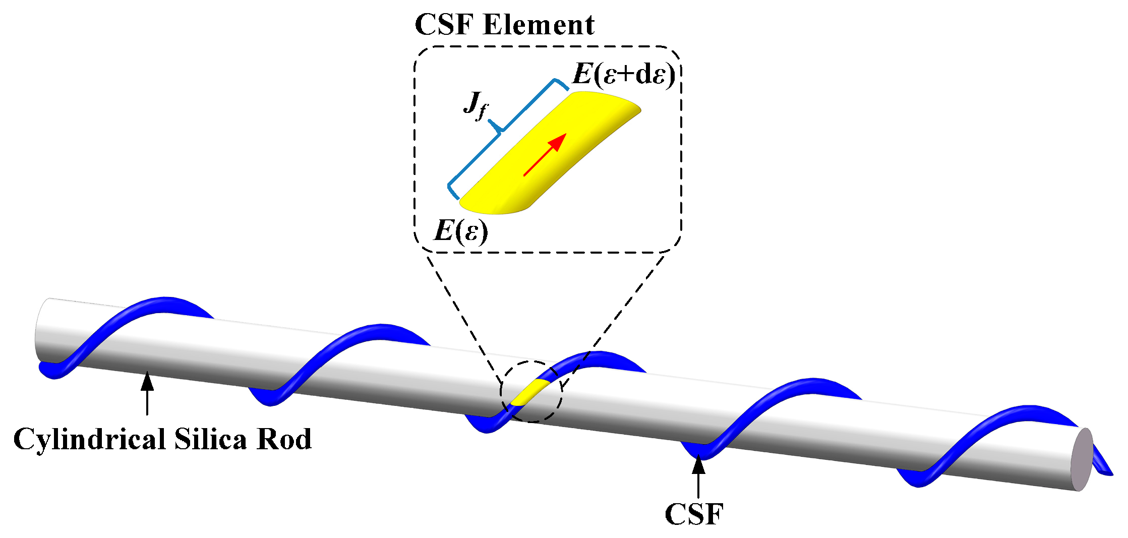
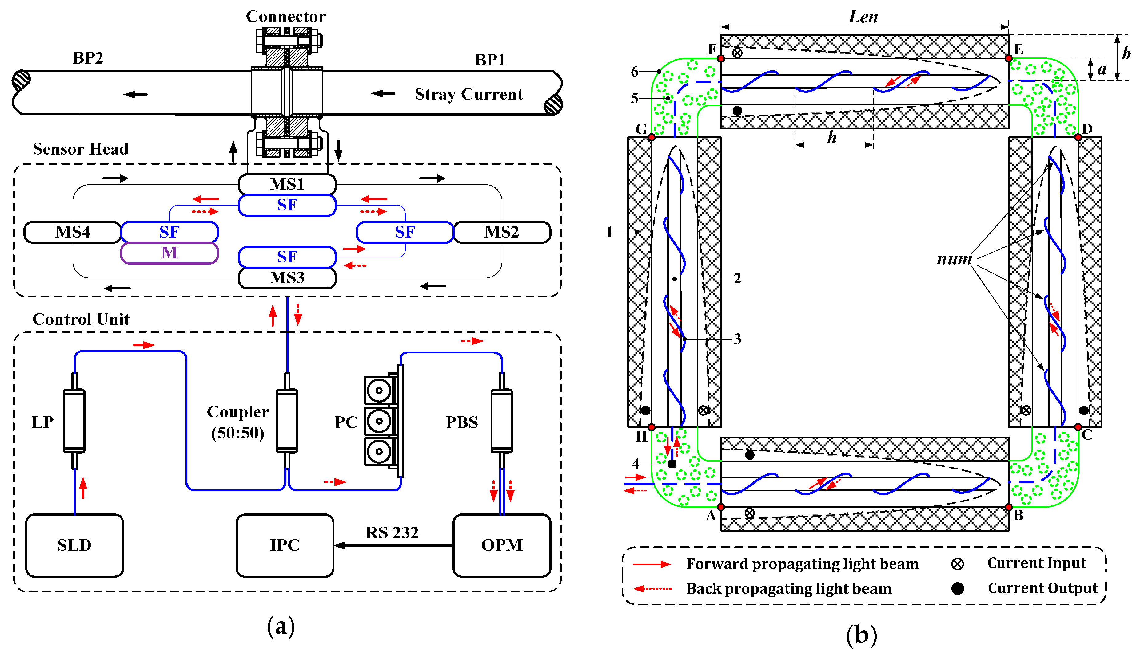
In our sensor, the circular birefringence is produced based on the geometric rotation effect [
17,
18]. This effect is described in that its polarization orientation will rotate and the rotation angle is equal to the integration of the torsion along the curve when the linearly polarized light propagates along the sensing fiber shaping into the non-planar curve. In the sections AB, CD, EF, and GH of the sensor head shown in
Figure 2b, the non-planar curves are all the cylindrical spiral curves. The sensing fiber is called the cylindrical spiral fiber (CSF) in this work. The parameter equation of the CSF can be given by
where
ε is the angle that makes a full circle, 0 ≤
ε ≤ 2π;
r is the radius of the cylindrical silica rod, mm;
num is the number of the curve spirals;
h is the length of each curve spiral, mm;
fx is equal to
rcos(
num·
ε);
fy is equal to
rsin(
num·
ε); and
fz is equal to (
h·
num·
ε)/(2π).
The torsion
τ and the curvature
μ of the CSF can be derived by
where
f’,
f’’ and
f’’’ represent the first derivative, the second derivative, and the third derivative, respectively; and (
f’,
f’’,
f’’’) represents the mixed product of
f’,
f’’, and
f’’’.
Moreover, the arc length of the infinitesimal vector
dl at
ε can be given by:
The magnetic field intensity on
dl can be simplified by [
12]
where
Cur is the stray current applied on the solenoid;
c is defined as
Len/2; and
n1 and
n2 are equal to
N1/
Len and
N2/(
b–
a), respectively. Among them,
a and
b represent the internal and external diameter of the solenoid, respectively.
Len represents the length of the cylindrical silica rod.
N1 and
N2 represent the number of turns of solenoid along the axial and vertical direction.
Since the CSF element
dl is infinitesimal, the linear birefringence, circular birefringence and Faraday rotation angle are distributed evenly in
dl. Thus, for the forward propagating light beam, the Jones matrix of the CSF element can be obtained as
where
q is equal to LB/2; LB represents the linear birefringence per unit length, rad/m;
V is the Verdet constant of the sensing fiber, which is about 0.73 μrad/A at 1550 nm [
7]. Since the CSF is wound on a cylindrical silica rod, the LB includes the bending-induced linear birefringence (BILB). Because the bending radius can be measured, the BILB per unit length is usually obtained as [
19]
where,
λ is the wavelength of the input light,
λ = 1.55 µm;
n is the refractive index of the fiber core,
n = 1.458;
p11,
12 are the strain-optical coefficients,
p11 = 0.121 and
p12 = 0.270;
ν is the Poisson’s ratio,
ν = 0.17;
κ is the equivalent radius of the sensing fiber,
κ = 62.5 µm;
μ is the curvature of the CSF that can be calculated based on Equation (2).
It is known that the other component of the linear birefringence LB is the TILB when the stray current sensor works in varying temperature conditions. The TILB per unit length can be obtained as [
20]
where,
E1 is the Young’s modulus of the CSF,
E1 = 7.0 × 10
10 N/m
2; ∆
σ is the stress difference between the orthogonal principal axes of the CSF, which is obtained as
where,
E2 is the Young’s modulus of the cylindrical silica rod,
E2 =
E1 in this work;
η is the linear expansion coefficient of the cylindrical silica rod,
η = 5.0 × 10
−7 /K;
T is the work temperature of the stray current sensor, which is within a range from −20 °C to 40 °C; and
T0 is the room temperature,
T0 = 20 °C. Thus, the LB of the CSF element is equal to (TILB + BILB)d
l.
For the back propagating light beam, the Jones matrix of the CSF element can be obtained as
The polarization evolution of the CSF element is shown in
Figure 3. For the forward propagating light, the complex amplitude of the input vector is assumed as
E(
ε) = [
Ex(
ε);
Ey(
ε)] while the complex amplitude of the output vector is assumed as
E(
ε + d
ε) = [
Ex(
ε + d
ε);
Ey(
ε + d
ε)]. According to the Jones calculus and Equation (5), the differential equations can be obtained as
A similar approach can be taken for the back propagating light. The complex amplitude of the input vector is assumed as
A(
ε) = [
Ax(
ε);
Ay(
ε)] while that of the output vector is assumed as
A(
ε + d
ε) = [
Ax(
ε + d
ε);
Ay(
ε + d
ε)]. The differential equations can be obtained as
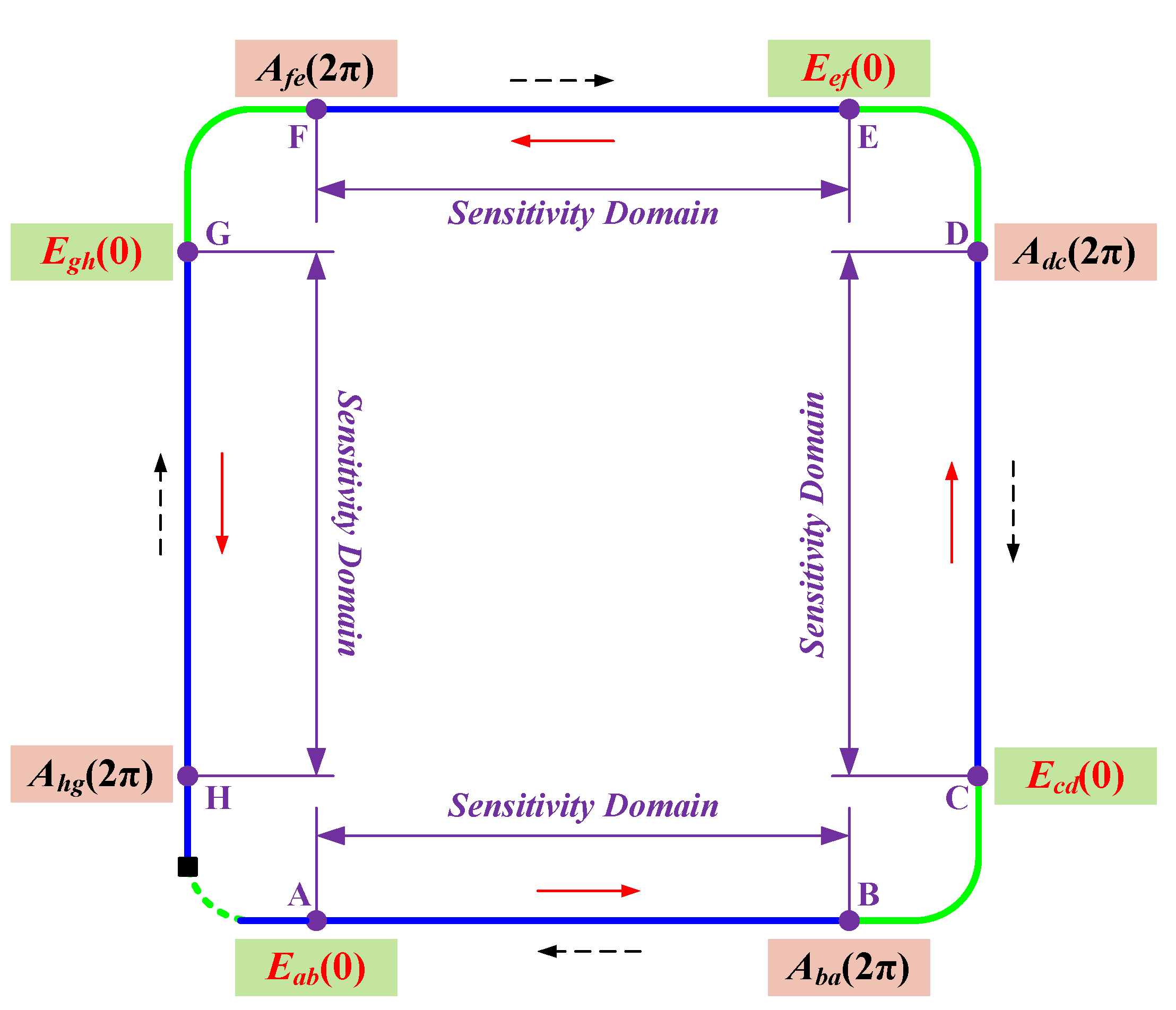
Figure 4 shows the initial condition of the differential equation of the CSF in each section. For the forward propagating light beam in section AB, the complex amplitude of the input vector is known at point A (
ε = 0), which is defined as
Eab(0). The differential equation shown in Equation (10) is calculated based on this known condition. According to the calculation result, the complex amplitude of the output vector can be obtained at point B (
ε = 2π), which is defined as
Eab(2π). Since the sensing fiber in section BC is short and freely placed, the polarization of light is considered to be unchanged. Thus, in section CD, the complex amplitude of the input vector at point C is the same as
Eab(2π), which is defined as
Ecd(0). Referring to the calculation method of
Eab(2π), the complex amplitude of the output vector can be obtained at point D, which is defined as
Ecd(2π). Similarly,
Eef(0),
Eef(2π),
Egh(0), and
Egh(2π) are obtained. Moreover, for the back propagating light beam,
Ahg(2π),
Ahg(0),
Afe(2π),
Afe(0),
Adc(2π),
Adc(0),
Aba(2π) and
Aba(0) are obtained in turn based on Equation (11). It is noted that
Ahg(2π) is the product of
Egh(2π) and
Jm that is the Jones matrix of the mirror.
Considering the sensor configuration presented in
Figure 2a, the complex amplitudes of the orthogonal vectors from PBS can be obtained based on
Aba(0) and
Jpc that is the Jones matrix of PC. The corresponding power signals after detection with OPM are defined as
Sx and
Sy. Applying the quadrature processing [
21], a sensor output
S is obtained as (
Sx −
Sy)/(
Sx +
Sy).
It is known that the expected output is obtained in the case that the linear birefringence is completely suppressed by the induced circular birefringence. In the expected case, the equivalent Jones matrix of the CSF in each section can be given by
where
F is the Faraday rotation angle,
F =
VHl. The total length
l of the CSF in each section can be derived as
Thus, in the expected case, the Jones matrix of the sensor head shown in
Figure 2a can be given by
On this basis, referring to the calculation of the
S, the expected output can be obtained, which is defined as
S0. The output error of stray current sensor can be given by Equation (15), which is defined as
U. According to the output error requirement proposed by Guangzhou metro, the
U caused by the linear birefringence should be smaller than 0.5% in the stray current measurement.
4. Parameter Optimization of the CSF
The known parameters of our sensor head include: a = 30 mm; b = 70 mm; n1 = 400 /m; n2 = 400 /m; r = 2 mm. The unknown key parameters are Len and num, respectively. The length of each curve spiral h is equal to the Len/num. Moreover, given our processing condition, Len is set within the range from 300 mm to 600 mm while num is set within the range from 1 to 64.
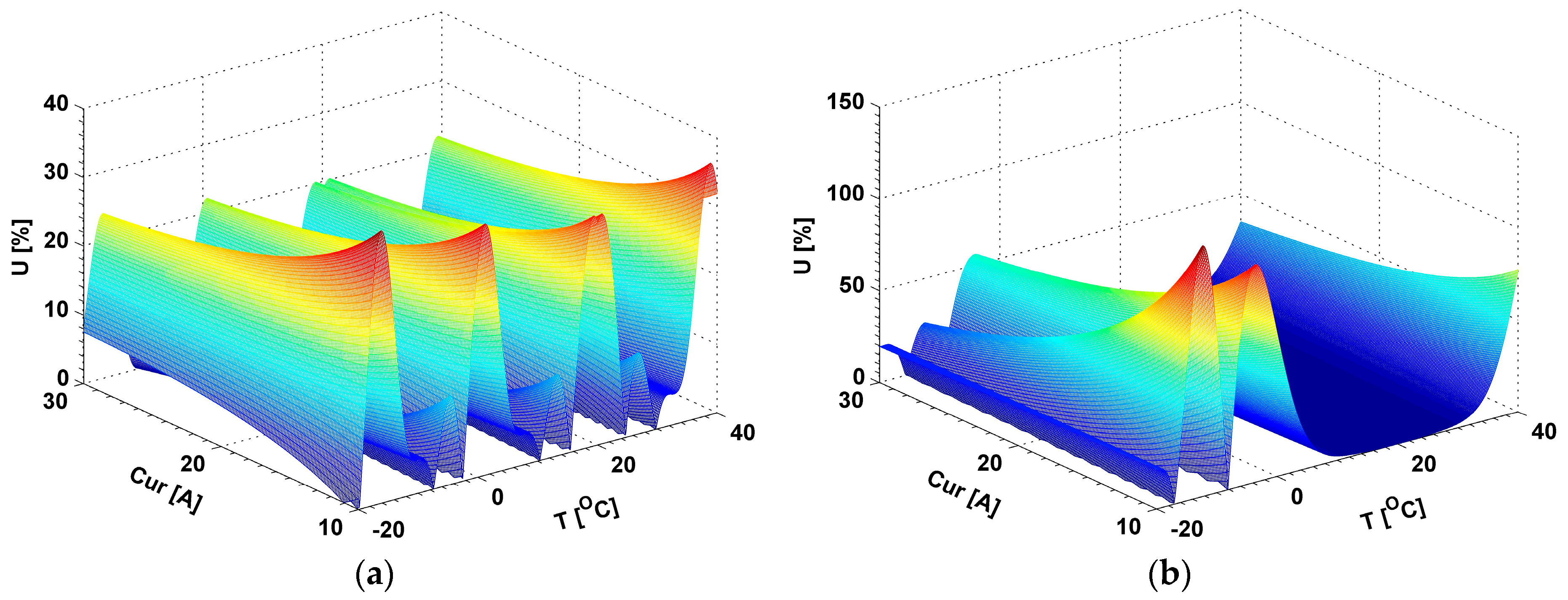
Two simulations have been conducted to evaluate the effect of these two unknown key parameters on the output error. During the simulations, the applied current (Cur) is set within the range from 10.0 A to 30.0 A based on our test results in Guangzhou metro, which is performed at 20 °C. The temperature is changed within the range from −20 °C to 40 °C. We define the total temperature-induced linear birefringence, the total bending-induced linear birefringence and the total circular birefringence of the CSF in each section as TTILB, TBILB, and TCB in this work. In the first simulation, the
Len is set as 600 mm and the
num is set as 64. According to Equation (13), the length of the CSF in each section is about 722 mm. According to Equations (7) and (8), the maximum TTILB is about 906 deg at −20 °C. According to Equation (6), the TBILB is about 8349 deg. Moreover, the torsion
τ can be obtained based on Equation (2), and the TCB is about 19139 deg. This simulation result is shown in
Figure 5a. The maximum U is about 39.6%. In the second simulation, the
Len and
num are set as 300 mm and 1, respectively. The length of the CSF in each section is about 300 mm. The TBILB, maximum TTILB, and TCB are about 0.0069 deg, 377deg, and 360 deg, respectively. The simulation result is shown in
Figure 5b. The maximum U is about 136.3%. In
Figure 5, it can also be found that the variation of the output error with the temperature changes in the first simulation is different from that in the second one. It indicates that the selections of these two unknown key parameters have a great influence on the output error. We believe obtaining the optimum results of these unknown parameters (
Len &
num) efficiently and accurately may be a challenge.
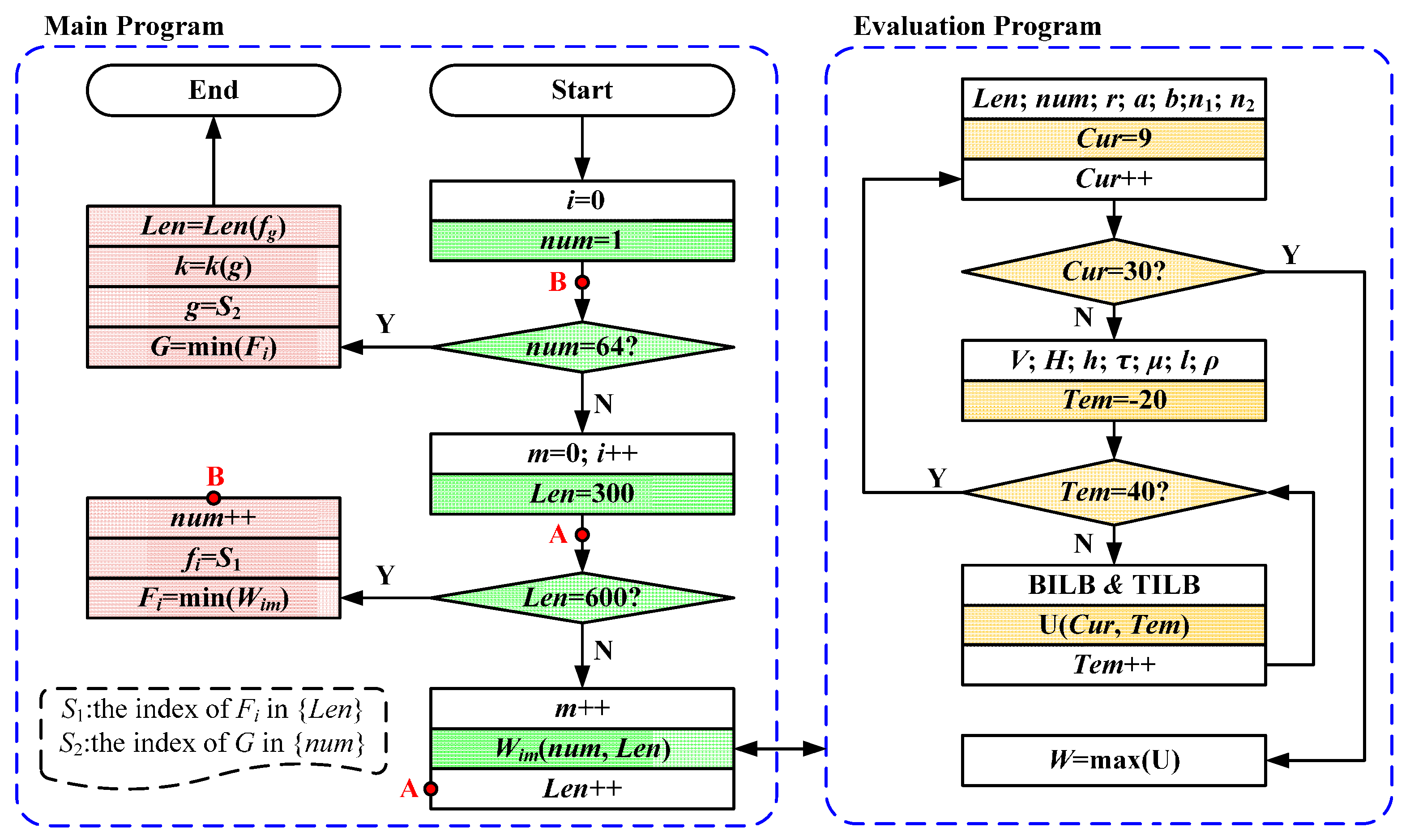
As far as we know, the optimum results are usually difficult to be obtained based on the common optimization algorithms, such as the genetic algorithm (GA) and the particle swarm optimization (PSO) algorithm. Thus, we proposed a direct search method to obtain the optimum results of the unknown parameters in this work. Compared with the GA or the PSO, our method can obtain the optimum results accurately, except for requiring more searching time. The flowchart of our method is shown in
Figure 6, which includes the main program and the evaluation program. The
num is searched within the range from 1 to 64 while the
Len is searched within the range from 300 to 600. The searching spaces of
num and
Len are defined as {
num} and {
Len}, respectively. In the main program, the evaluation function result
Wim can be obtained at the
ith
num and the
mth
Len. On this basis, there are two steps to obtain the optimum results of the unknown parameters. Firstly, at the
ith
num, the minimum result and its index in the {
Len} are obtained, which are defined as the
Fi and
S1. Secondly, the minimum results of {
Fi} and its index in the {
num} are obtained, which are defined as
G and
S2. Finally, the optimum results of
num and
Len can be found according to the indexes
S1 and
S2. Moreover, the evaluation program shows the physical structure of the evaluation function. At the
ith
num and the
mth
Len, the maximum output error can be calculated within the range of the stray current from 10 A to 30 A and of the temperature from −20 °C to 40 °C. In this work, we consider the maximum output as the evaluation function result at the
ith
num and the
mth
Len. It is noted that the theoretical bases of the evaluation program are Equations (1) to (15).
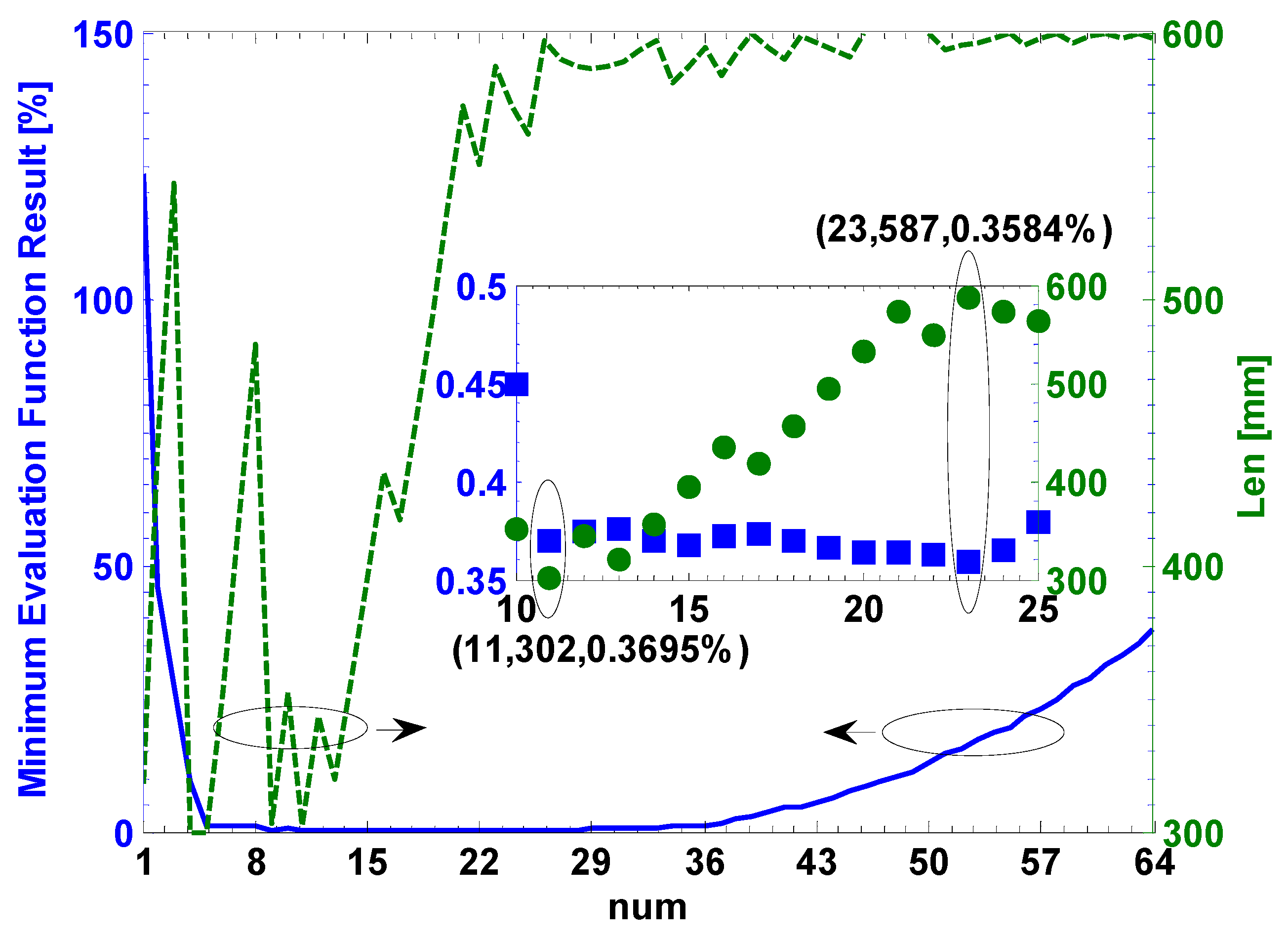
Figure 7 shows the minimum evaluation function result (MEFR) versus the unknown parameters (
num &
Len). The optimum results are that the
num is 23 and the
Len is 587 mm, where the MEFR is about 0.3584%. Moreover, the MEFRs in the range of the
num from 10 to 25 are compared, which is shown in the inserted picture of
Figure 7. It can be found that the MEFR is about 0.3695% when the
num is 11 and the
Len is 302 mm. Obviously, the MEFR in the latter case (about 0.3695%) can be little more than the optimum case (about 0.3584%). However, the two unknown parameters of the latter case are smaller than the optimum case, which may lead to the manufacture of the latter case being much easier. Thus, in this work, the unknown parameters
num and
Len are set as 11 and 302 mm, respectively.
In
Figure 7, the change of the MEFR includes three cases: firstly decreases when the
num increases from 1 to 9, then vibrates when the
num increases from 10 to 25, finally increases when the
num increases from 26 to 64.
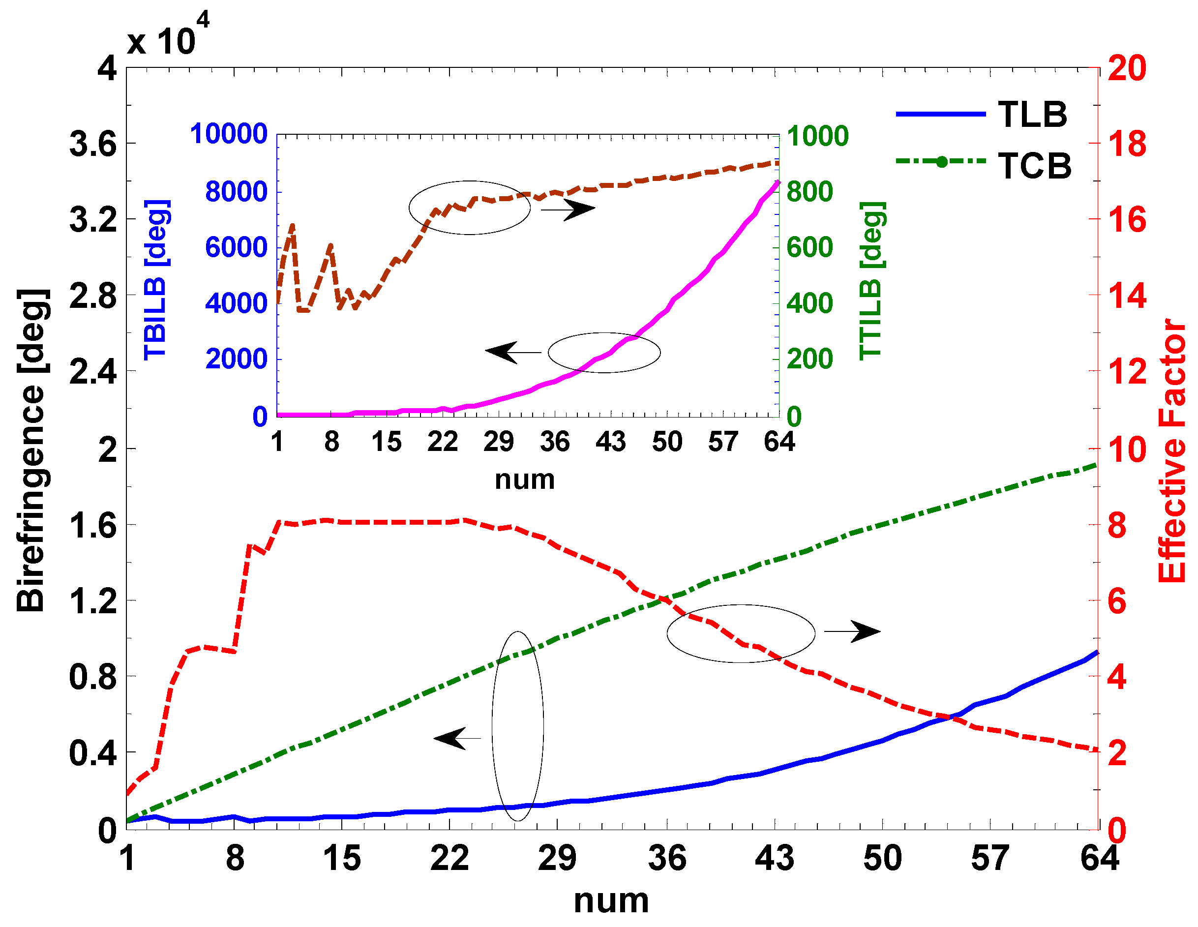
Figure 8 shows the birefringence and the effective factor versus the unknown parameters. The TBILB increases from 0.006 deg to 8407.1 deg while the maximum TTILB (at −20 °C) increases from 377.8 deg to 904.3 deg when the
num increases from 1 to 64. They are shown in the insert picture of
Figure 8. We defined the total linear birefringence of the CSF in each side as TLB. The maximum TLB is the sum of the TTILB and the TBILB, which increases from 379.6 deg to 9311.4 deg. Moreover, the TCB increases from 359.9 deg to 19119.2 deg. We proposed the effective factor (EF) to express the change of the MEFR, which is given by:
In the first case, the EF increases from 0.902 to 7.427 as the num increases. The MEFR decreases from 123.3% to 0.42%. In the second case, The EF vibrates within the range from 7.23 to 8.07 and the MEFR also vibrates within the range from 0.358% to 0.449%. Among them, the minimum MEFR is about 0.358% at num = 23 and Len = 302 mm when the EF is about 8.07. Finally, in the last case, the EF decreases from 7.93 to 2.05 and the MEFR increases from 0.372% to 37.96%. In this work, the MEFR is required to be smaller than 0.5%, which indicates that most of the linear birefringence should be suppressed by the circular birefringence produced by the CSF. Thus, the EF needs to be greater than 7.42.
From discussion above, the
num and the
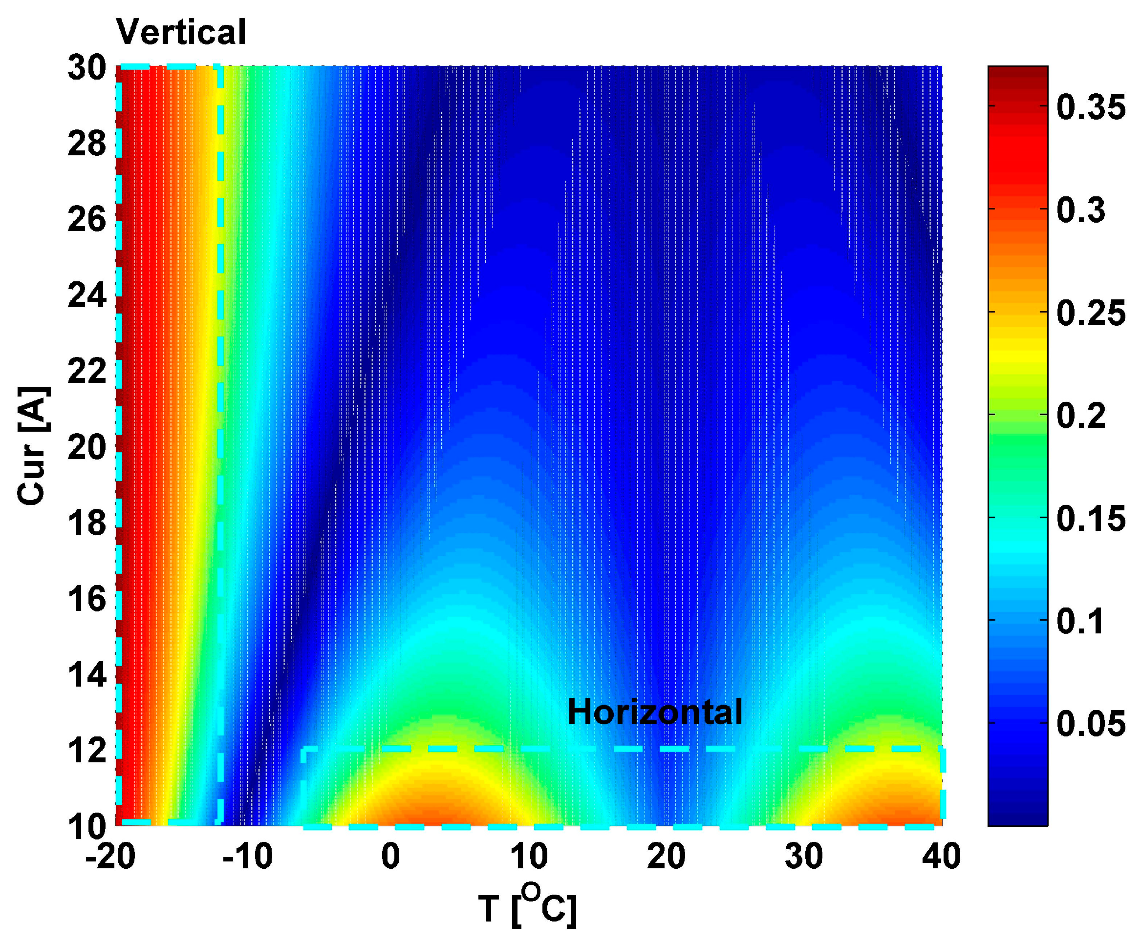
Len of the CSF in each side are set as 11 and 302 mm, respectively. The theoretical results using this CSF are calculated as follows: the length of the CSF in each section is about 309.8 mm; the TBILB, maximum TTILB, and TCB are about 92.33 deg, 388.78 deg, and 3860.2 deg, respectively. The EF using this CSF is not smaller than 8.02. Moreover, the output error distribution of our sensor using this CSF is shown in
Figure 9 when the Cur is changed within the range from 10.0 A to 30.0 A and the temperature (
T) is changed within the range from −20 °C to 40 °C. It can be found that the maximum output error is about 0.3695% as the temperature changes, which achieves the output error requirement that is not greater than 0.5%. In
Figure 9, we can also find that there are two sections with relatively large output error. The vertical section is caused in the range of the
T from −20 °C to −17 °C, where the TILB is relatively large. The horizontal section is caused in the low stray current range of about 10.0 A to 12.0 A. It is noted that the Faraday effect induced by the applied stray current can be considered as the circular birefringence [
20], which is proportional to the applied stray current. Therefore, at the same temperature condition, most of the linear birefringence can be suppressed by the circular birefringence induced by the CSF, the effect of the residual linear birefringence that is not suppressed may be more significant in the low current (10.0 A to 12.0 A) than the high current (≥12.0 A), which is due to the low Faraday effect in the low current.
5. Verification Test
According to the discussion above, the linear birefringence and the circular birefringence work together in the CSF. It is a complex measurement problem and there are no accurate methods to measure the mutual coupling birefringence in the meter-long CSF at present. Thus, the direct measurement on the linear or circular birefringence cannot be performed in this work. The other verification method is applied, that is, the temperature experiments are conducted to verify the feasibility and effectiveness of the CSF. In the temperature experiments, the SLD and the OPM are both produced by EXFO Co. Ltd. (mode FLS-2200 and PM-1623, Quebec, QC, Canada). The 3 dB spectral width of SLD is about 56 nm. The extinction ration of LP is about 35 dB and that of PBS is about 31 dB. The coupling ratio of coupler is about 50:50. Moreover, it is noted that the detection result of a digital multimeter (Agilent Co. Ltd., model U3402A, Santa Clara, CA, USA) is used as the standard value of the experiment current. Accuracies for the DC current and voltage are 0.05% and 0.012%, respectively. The corresponding measuring ranges are smaller than 12 A and greater than 120 mV. If the experiment current is greater than 12 A, a precision shunt (type 25A/250 mV) will be required. The parameters of the CSF in each side are summarized as follows: the radius of the cylindrical silica rod is about 2 mm; the length of the cylindrical silica rod is about 302 mm; the number of the curve spirals is about 11; the CSF is the low-birefringence fiber, where the inherent linear birefringence is about 4 m/4° (Oxford Electronics Co. Ltd., model LB 1550-125, Hants, UK).
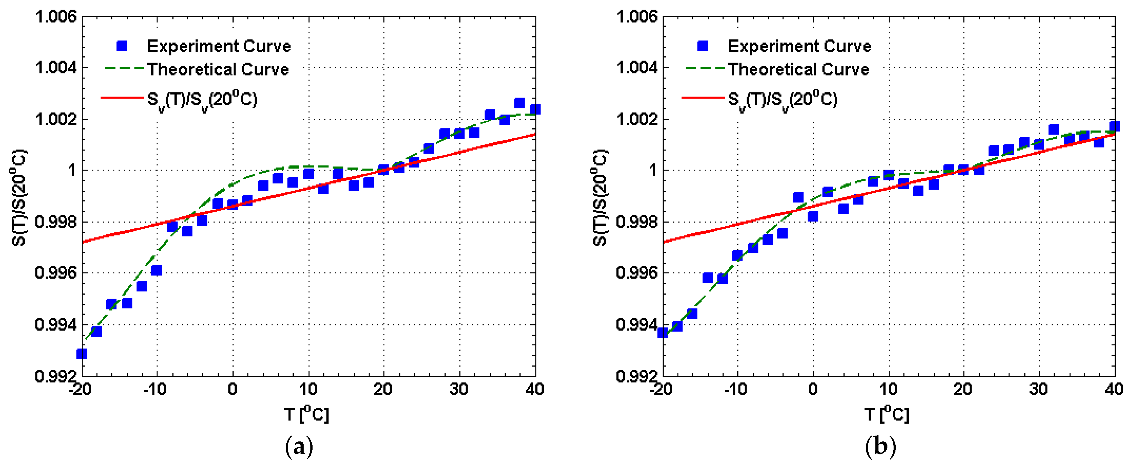
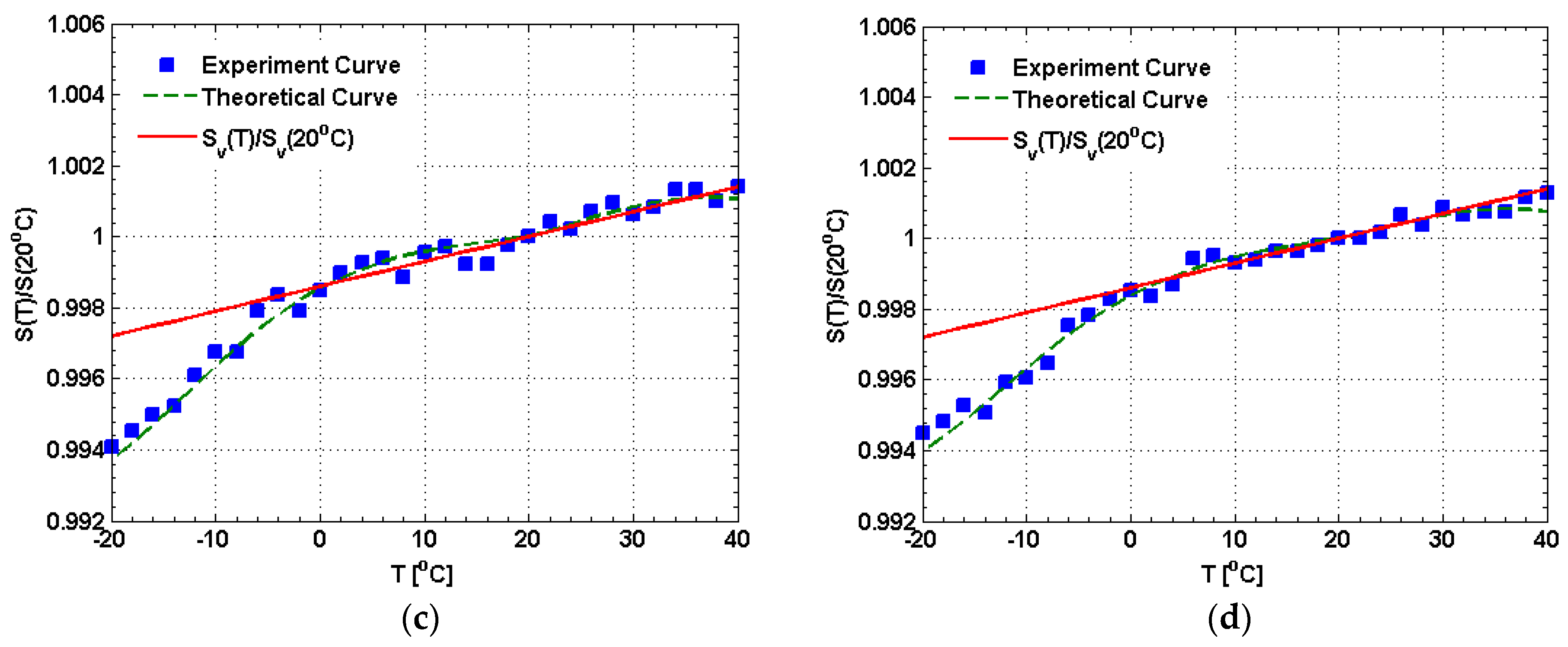
During the following temperature experiments, the sensor output is measured as a function of temperature, for different input current. The temperature experiments are conducted by adjusting the temperature of sensor head from −20 °C to 40 °C based on a high-low temperature test chamber. The sampling is carried out every 2 °C. The temperature experiment results are shown in
Figure 10, which are all normalized to the sensor output at 20 °C. For example, the normalized output at 20 °C is equal to 1. If the linear birefringence is suppressed completely by the circular birefringence produced by the CSF, the temperature dependence of the stray current sensor will arise primarily through the change in the Verdet constant with temperature. The normalized form (d
V/d
T)/
V0 can be used to represent the temperature dependence of the Verdet constant, where
V0 is the Verdet constant of the CSF at 20 °C. It is noted that the (d
V/d
T)/
V0 is about 7 × 10
−5/°C [
22]. Thus, only considering the temperature dependence of the Verdet constant in the case that the linear birefringence is suppressed completely, the normalized sensor output as the temperature changes can be expressed by
Thus, the error at some temperature is the difference between the normalized output at this temperature and that at 20 °C, including the first error caused by the temperature dependence of the Verdet constant and the second error caused by the linear birefringence. Among them, the first error can be obtained based on Equation (17).
Figure 10a–d are obtained at 15.0, 20.0, 25.0, and 30.0 A, respectively. It can be found that the experiment curves gradually trend to the temperature dependence curve based on Equation (17) as the input current increases, especially within the range of the temperature from 0 °C to 40 °C. It means that the effect of the linear birefringence can be eliminated more effectively as the input current increases, which is consists with the discussion of the horizontal section in
Figure 9. In
Figure 10a, excluding the contribution of the temperature dependence of the Verdet constant (the first error), the maximum second error is occurred at −20 °C that is about 0.43% compared with 20 °C. Similarly, in
Figure 10b–d, the maximum second error is about 0.35%, 0.33%, and 0.32%, which all occurred at −20 °C. These results indicate that the effect of the most of the linear birefringence can be eliminated effectively by the circular birefringence produced by the CSF. The measurement error caused by the linear birefringence can be controlled at less than 0.43% which achieves the output error requirement (≤0.5%). It is noted that the temperature dependence of the Verdet constant (the first error) can be compensated based on the neural network or database technology, which will be our future work.

