A Quantitative Comparison of Calibration Methods for RGB-D Sensors Using Different Technologies


Abstract
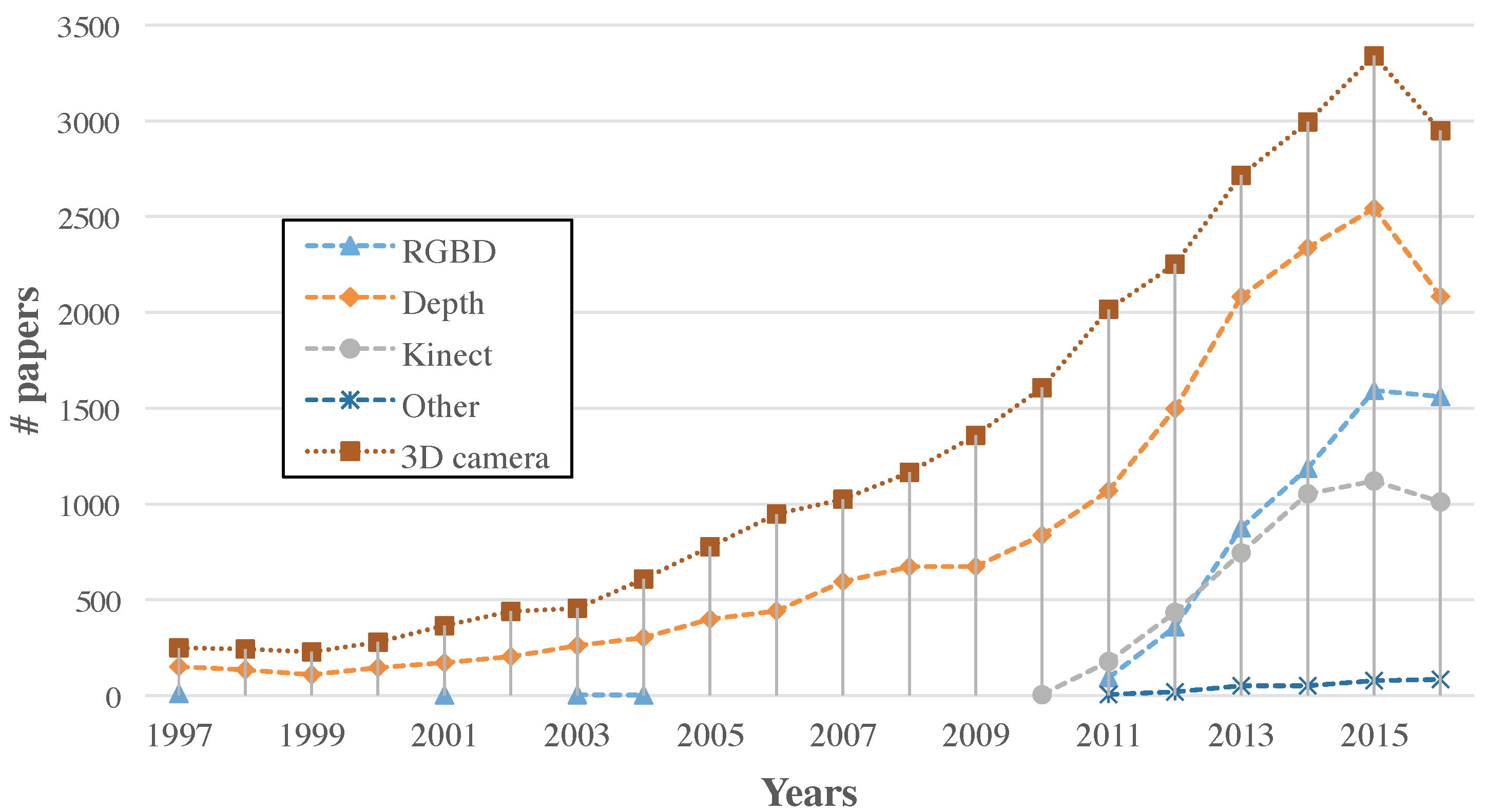
:1. Introduction
- Contact devices. They need a direct contact with the subject of interest to provide 3D information.
- Contactless devices. They are able to provide 3D information from the distance.
- Passive methods measure the scene radiance as a function of the object surface and environment characteristics using (usually) non-controlled ambient light external to the imaging system. Hence, only visible features of the scene are measured, providing high accuracy for well-defined features, such as targets and edges. However, unmarked surfaces are hard to measure [9]. In this category, techniques such as shape-from-X (e.g., shading, defocus, silhouettes, etc.), structure-from-motion and stereo are included. Stereo vision has received significant attention over the past decade in order to provide more accurate results and obtain them faster [10]. Usually, the methods use two or more calibrated RGB cameras to get the depth image by computing the disparity information from the images that conform to the system [11]. Stereoscopic cameras have been used for many purposes, including 3D reconstruction [12]. This technology can provide both colour and depth information, but it is required to be calibrated every time its location is changed, making its portability more difficult. Besides, they need the presence of texture to obtain the 3D information. In some devices, the distance between both cameras could be changed to fit the working range of the system.
- Active methods use their own light source in the imaging system for the active illumination of the scene [13]. The sensor is usually focused on known features from this light source. Then, the illumination and the features are designed to be easily measured in most environments. Since they have difficulties with varying surface finish or sharp discontinuities such as edges [9], compared with the passive approach, active visual sensing techniques are in general more accurate and reliable [14]. Active sensors could be classified into two broad categories [15]: triangulation and time delay. The former rely on the triangulation principle using the light system, the scene and the sensor. The main differences between the methods include the nature of the controlled illumination (laser or incoherent light) and its geometry (beam, sheet, or projected pattern). Laser triangulators, structured light and moiré methods are examples that fall into this level. Time delay systems measure the time between emission and detection of light reflected by the scene (Time-of-flight, ToF) or the phase difference between two waves (Interferometry). Focusing on the ToF, pulsed-light and continuous wave modulation are the technologies available nowadays. Pulsed-light sensors directly measure the round-trip time of a light pulse. In order to obtain a range map, they use either rotating mirrors (LIDAR - Light Detection and Ranging o Laser Imaging Detection and Ranging) or a light diffuser (Flash LIDAR). LIDAR cameras usually operate outdoors and their range can be up to a few kilometers. Continuous wave sensors measure the phase difference between the emitted and received signals and usually operate indoors. Thier ambiguity-free range is usually fixed from 30 cm to 7 m [16,17]. A extensive comparison of ToF technologies can be found in [18].
2. Materials and Methods
2.1. RGB-D Cameras
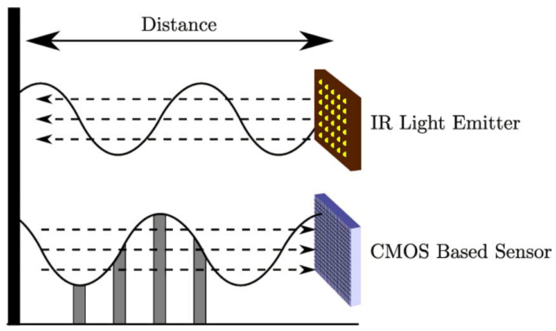
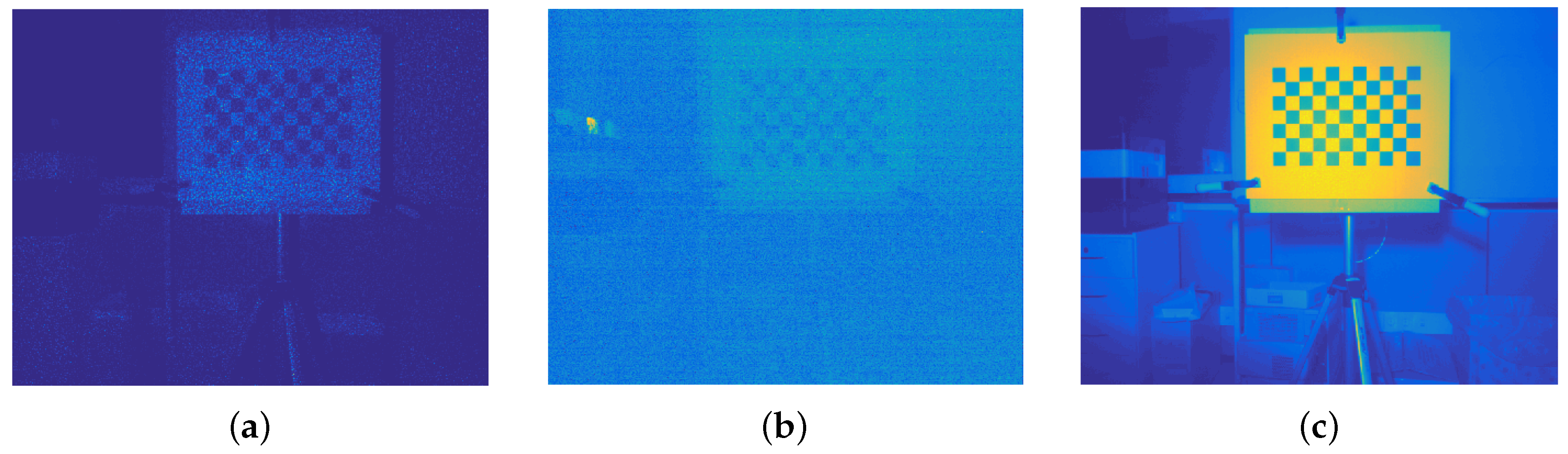
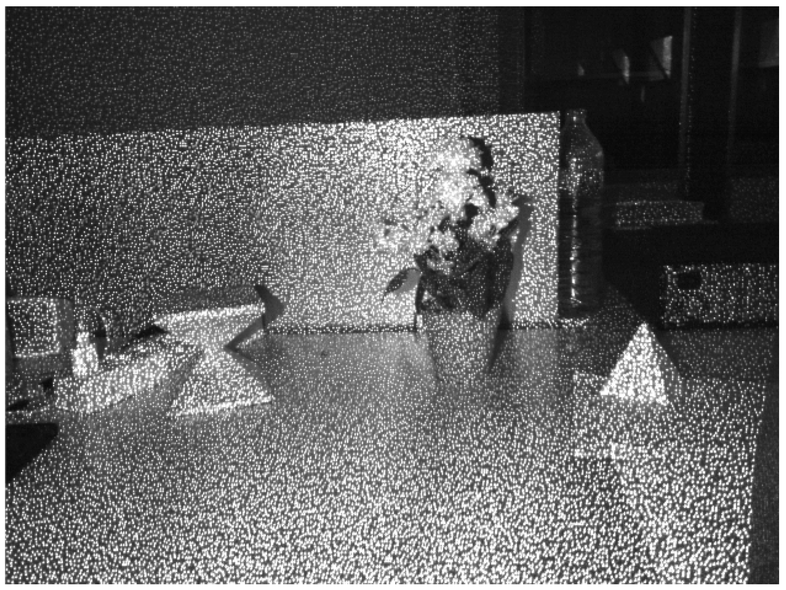
- Structured Light (SL) based sensors are composed of a near-infrared emitter and an infrared (IR) camera. The infrared emitter projects a known pattern over the scene, simultaneously the IR camera gets the pattern and computes the disparity between the known and the observed pattern [42,43,44]. Usually, the infrared is chosen as the bandwidth of the projected pattern to avoid interfering with visible light in the scene. Nevertheless, a drawback of this technology is the impossibility of working in places where the illumination hinders the perception of the pattern [45]. More information about this technology can be found in [20]. For example, consumer RGB-D as Microsoft Kinect, Asux Xtion Pro or PrimeSense Carmine use structured light by projecting a speckle pattern over the scene (see Figure 2).
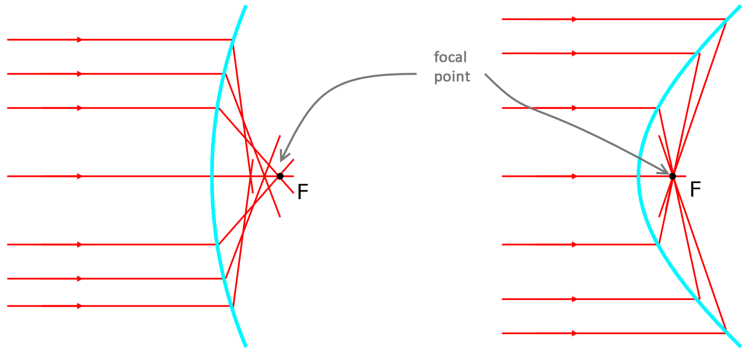
- Time-of-Flight (ToF). As has previously been stated, ToF sensors obtain the distance to a subject of interest by measuring the time between the emission of a signal and its reflection from the subject. Consumer cameras that use this technology are based on a continuous wave sensor combined with a calibrated and internally synchronized RGB camera. A near-infrared emitter emits incoherent light, which is a modulated signal with a frequency ω. This light incises in the scene, producing a reflected signal with a phase shift with respect to the emitted signal (see Figure 3). Hence, the distance is given by the Equation (1), where c is the speed of light [46]. Microsoft Kinect V2 is the best representative example of this kind of cameras, achieving one of the best image resolutions among ToF cameras commercially available and an excellent compromise between depth accuracy and phase-wrapping ambiguity [18].
2.2. Camera Calibration Parameters
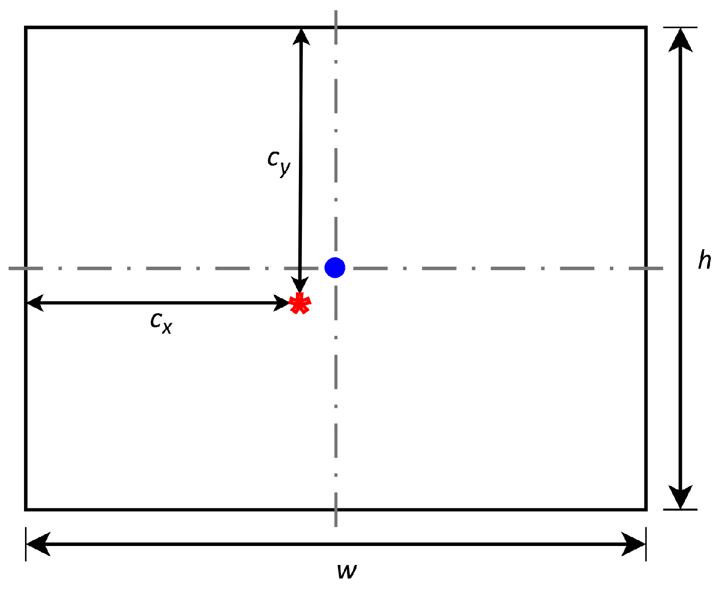
2.2.1. Intrinsic Parameters
2.2.2. Extrinsic Parameters
2.3. Calibration Methods
2.3.1. Bouguet Method
2.3.2. Burrus Method
2.3.3. Herrera Method
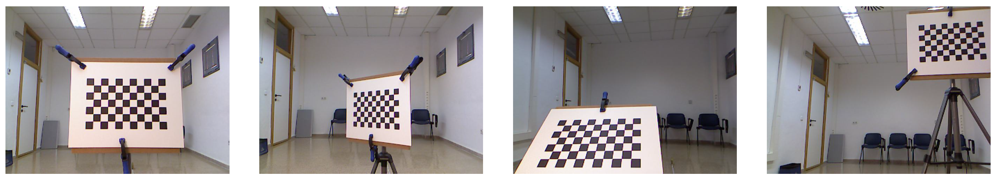
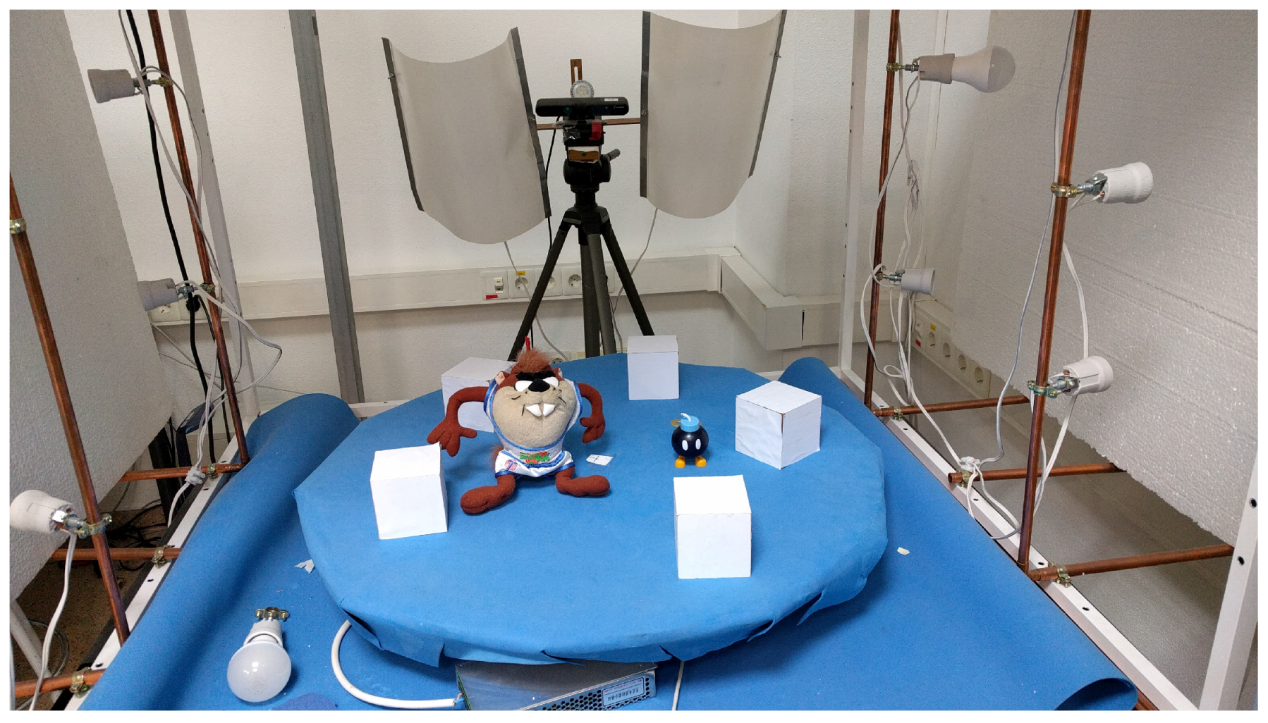
3. Experimentation
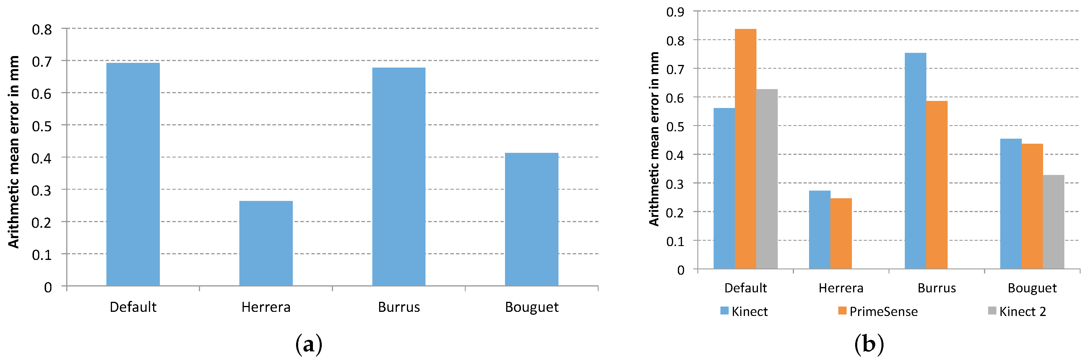
3.1. Calibration Results
3.2. Experimental Results
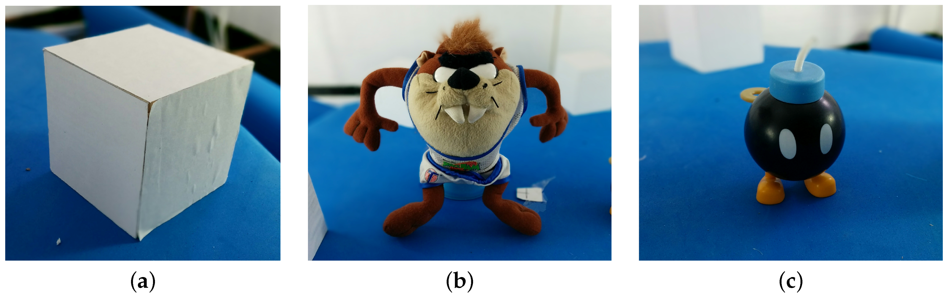
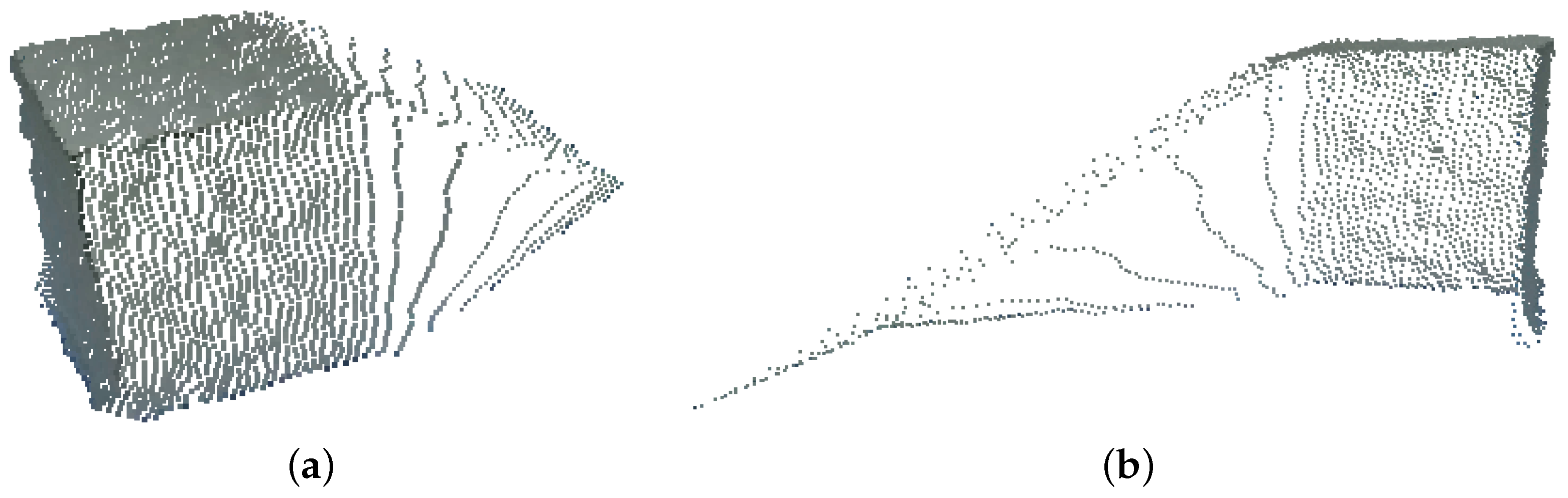
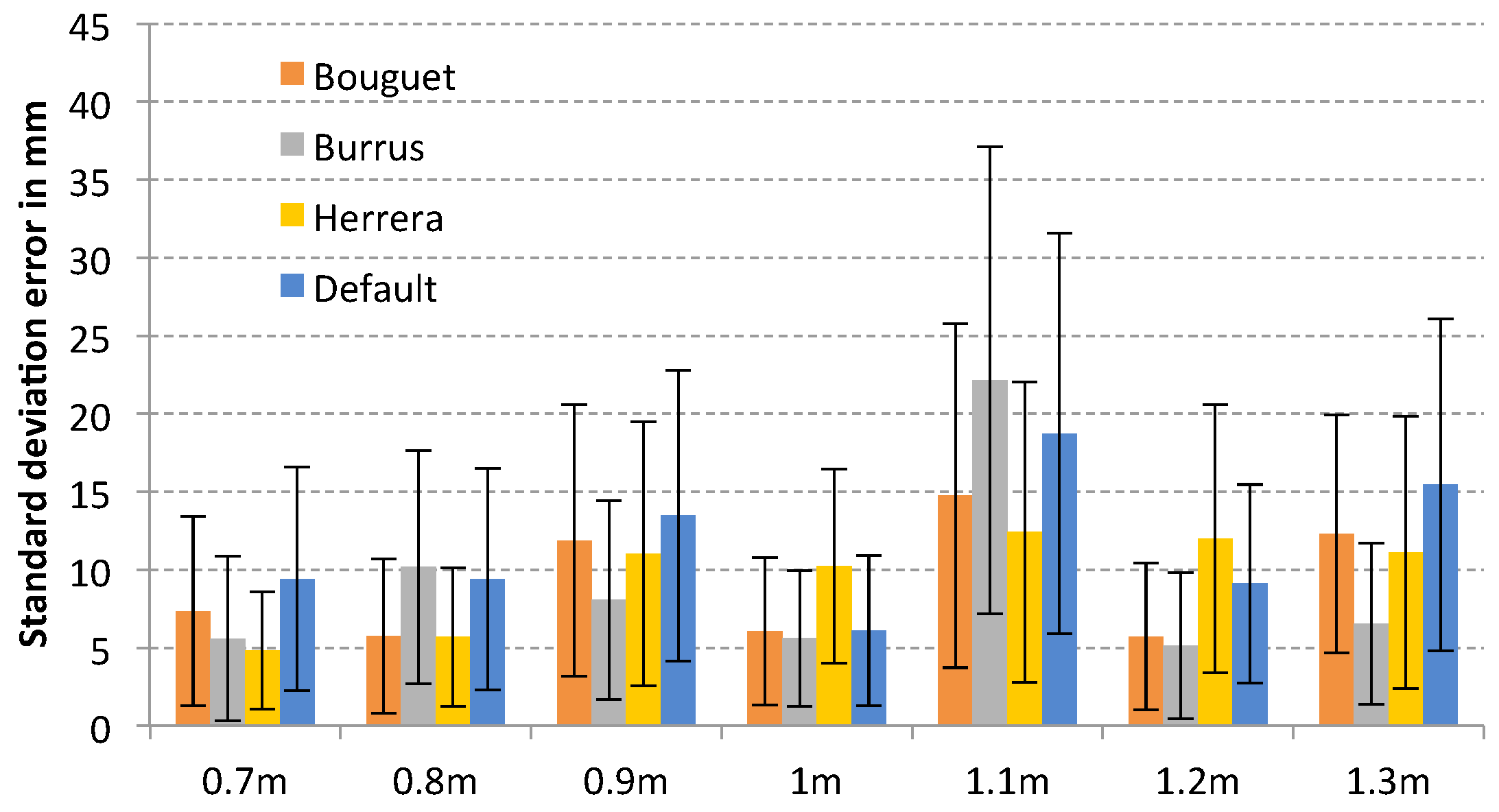
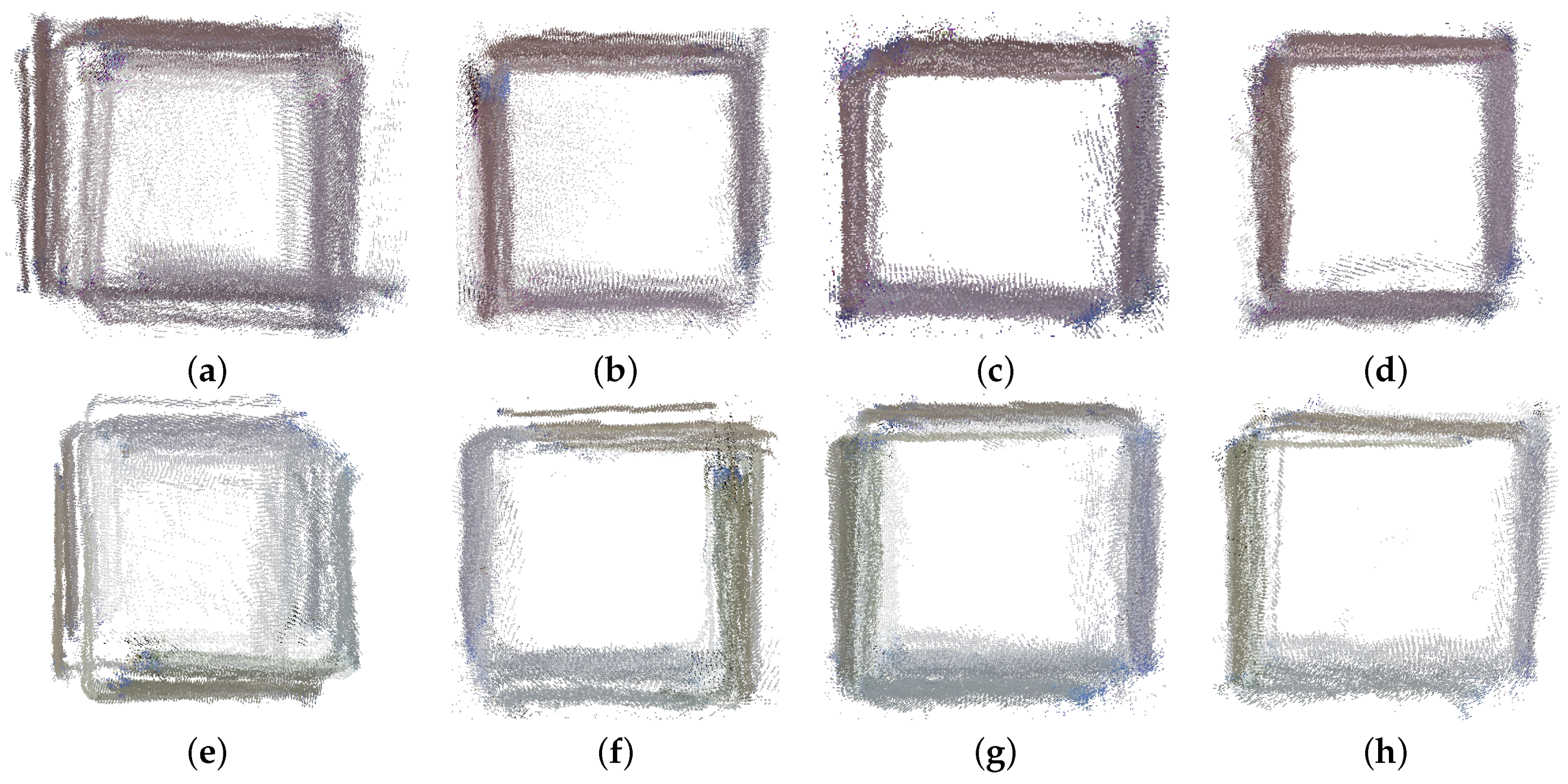
3.2.1. Plane Fitting Test
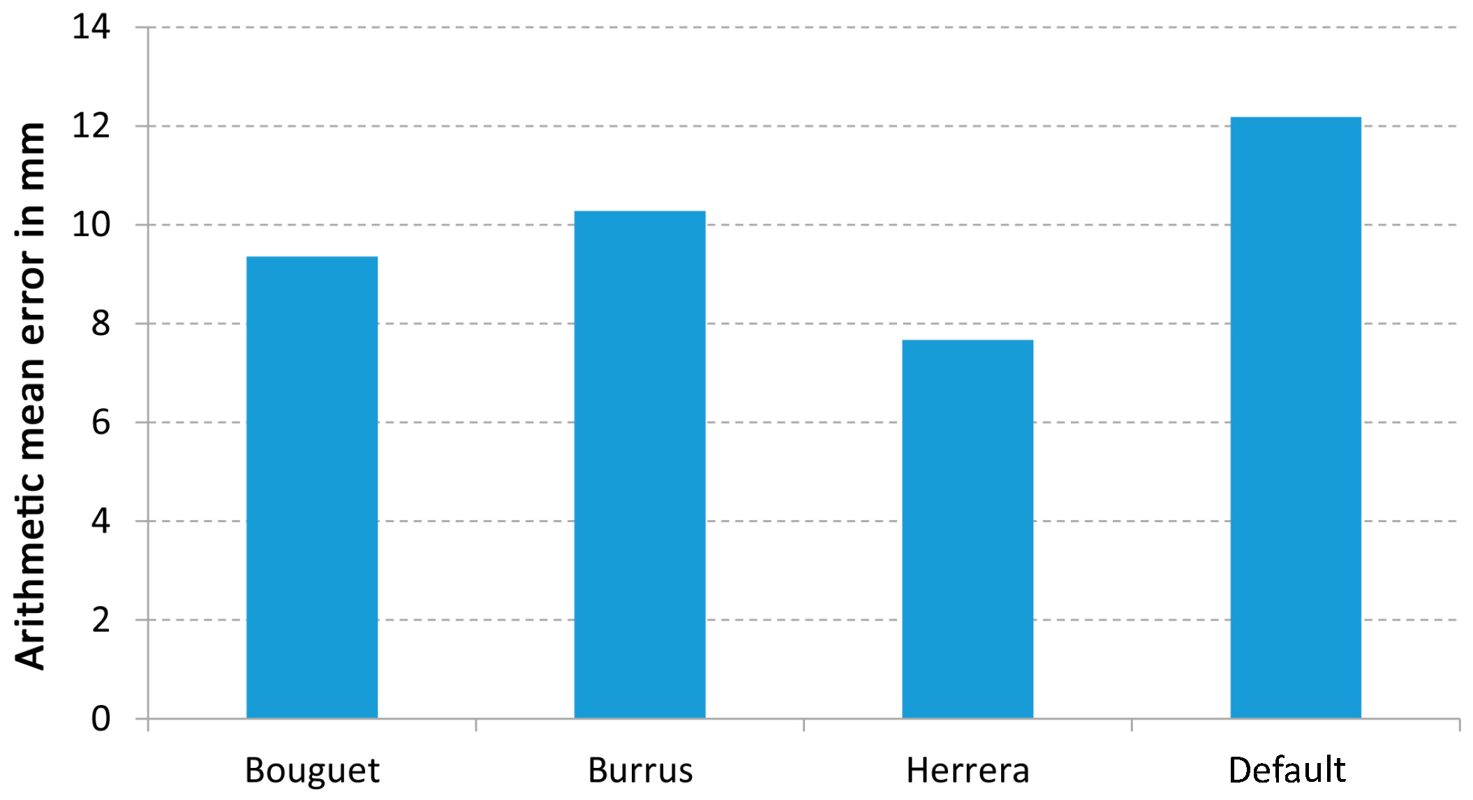
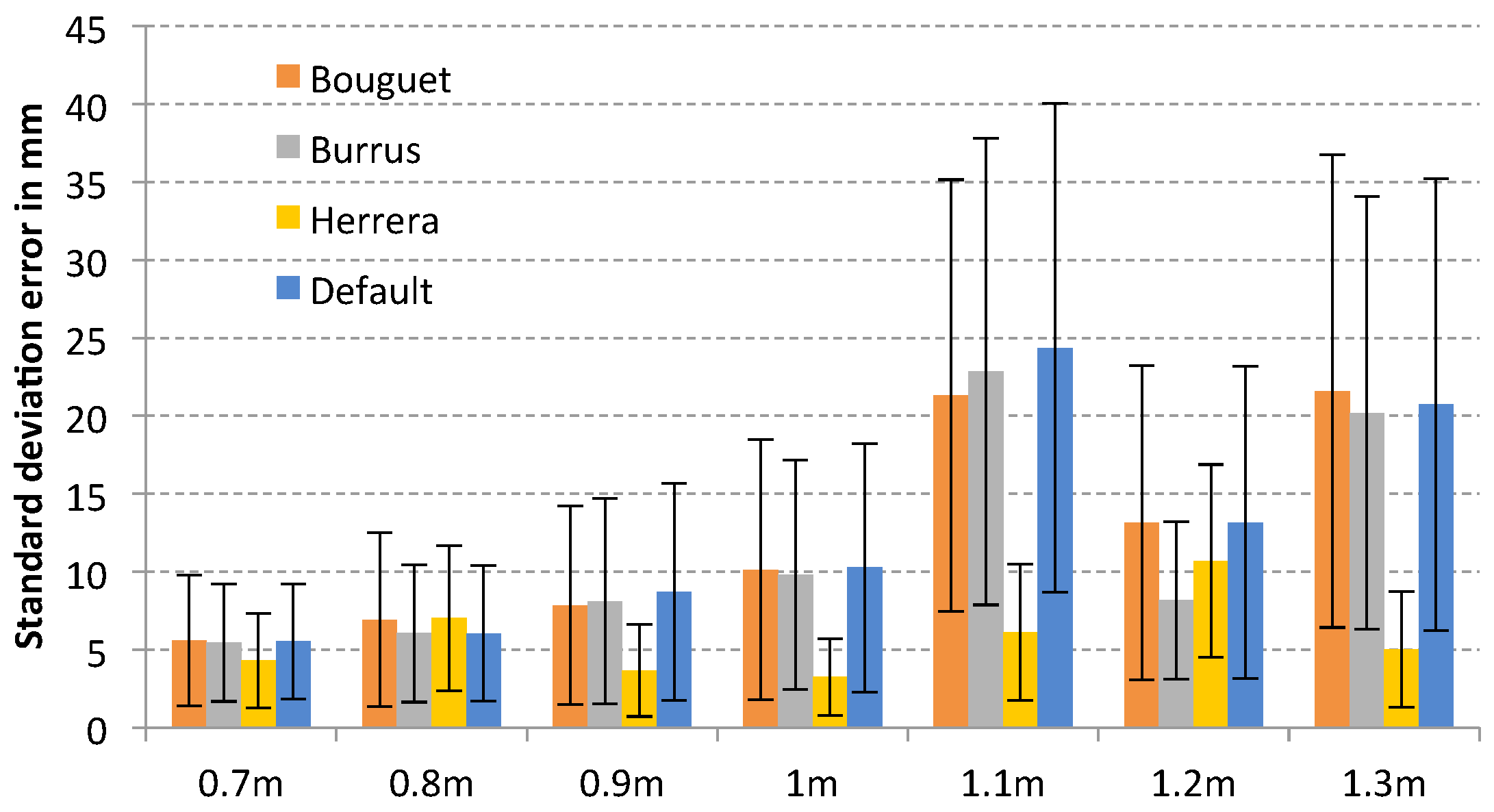
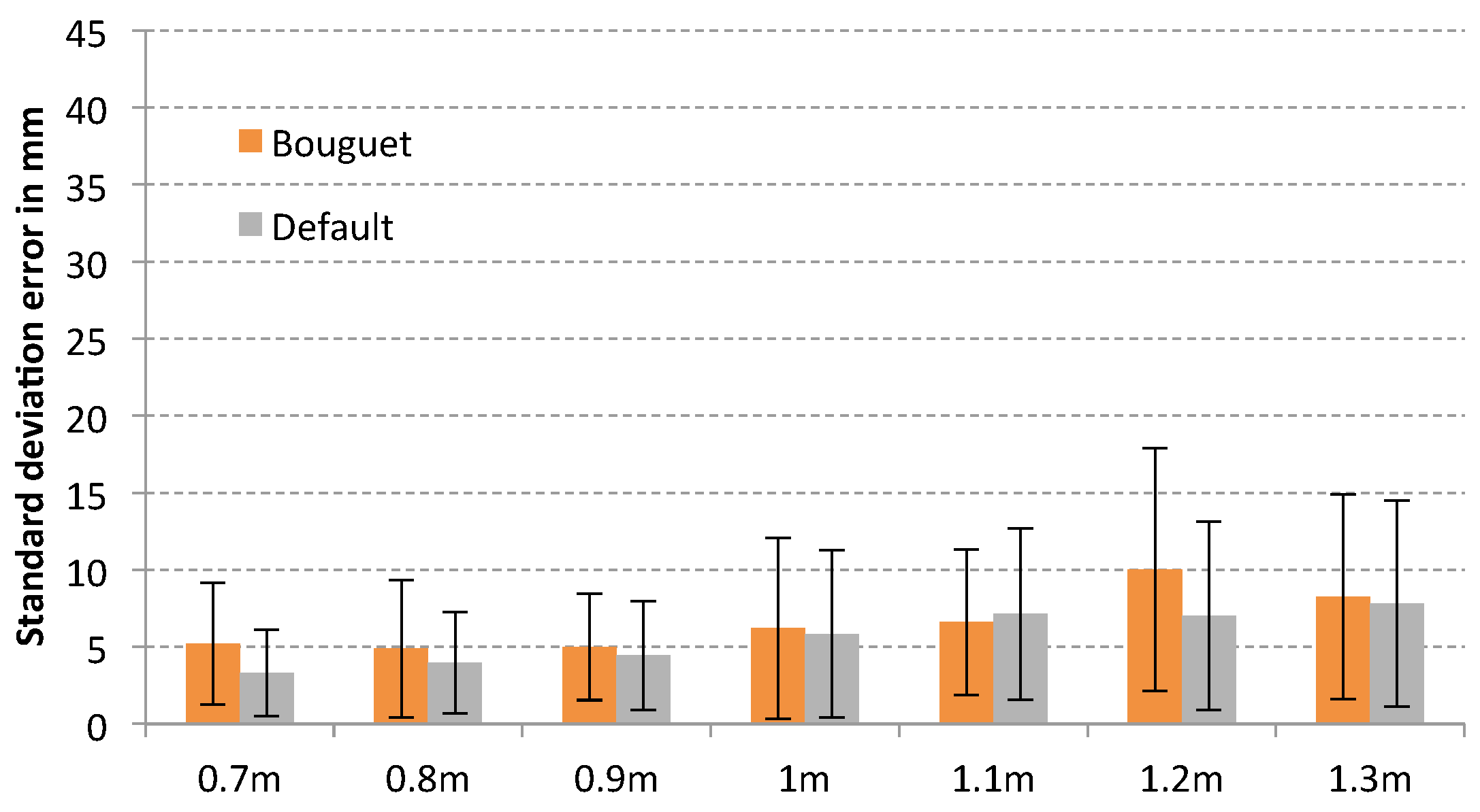
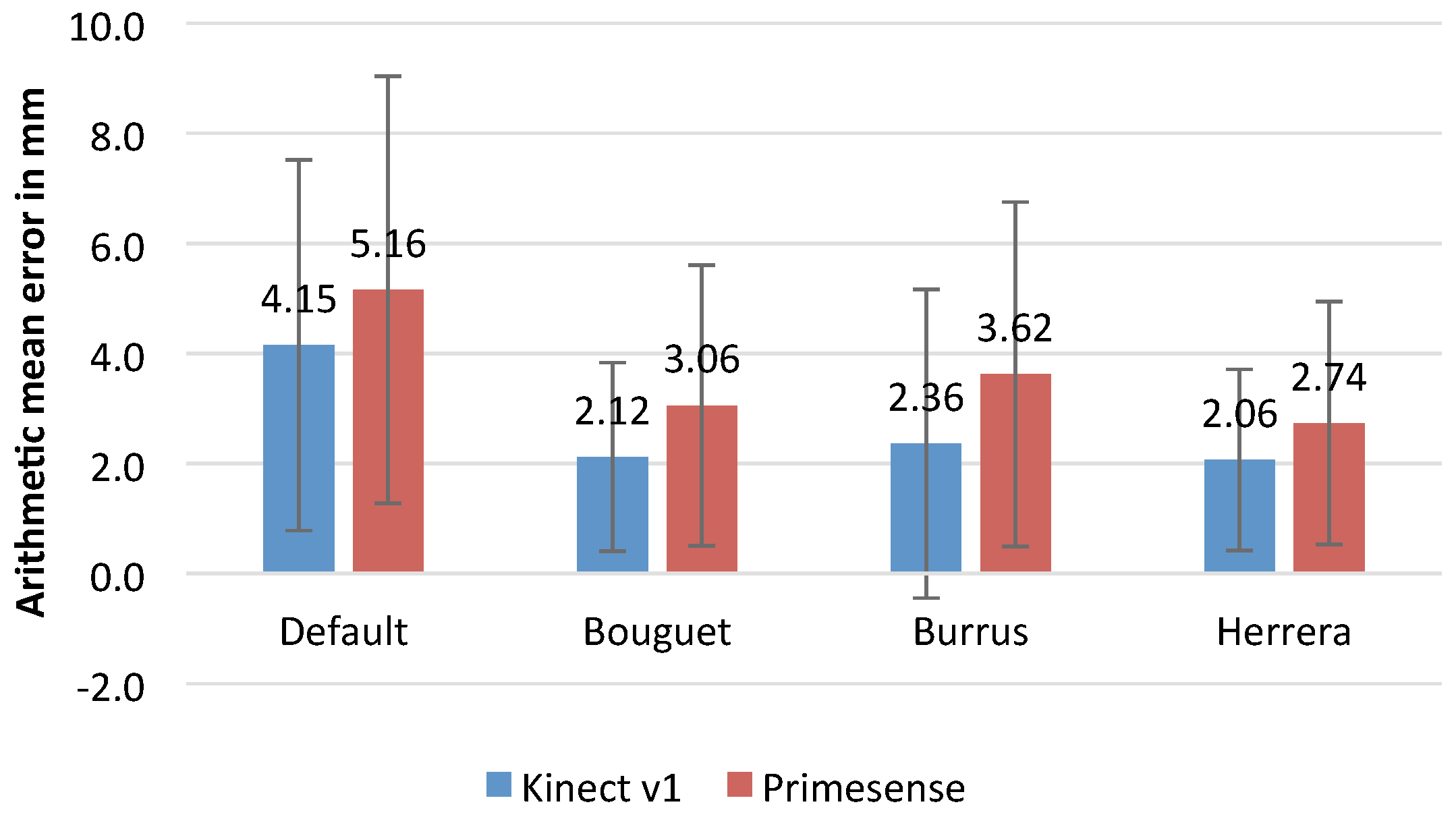
3.2.2. Measurement Error
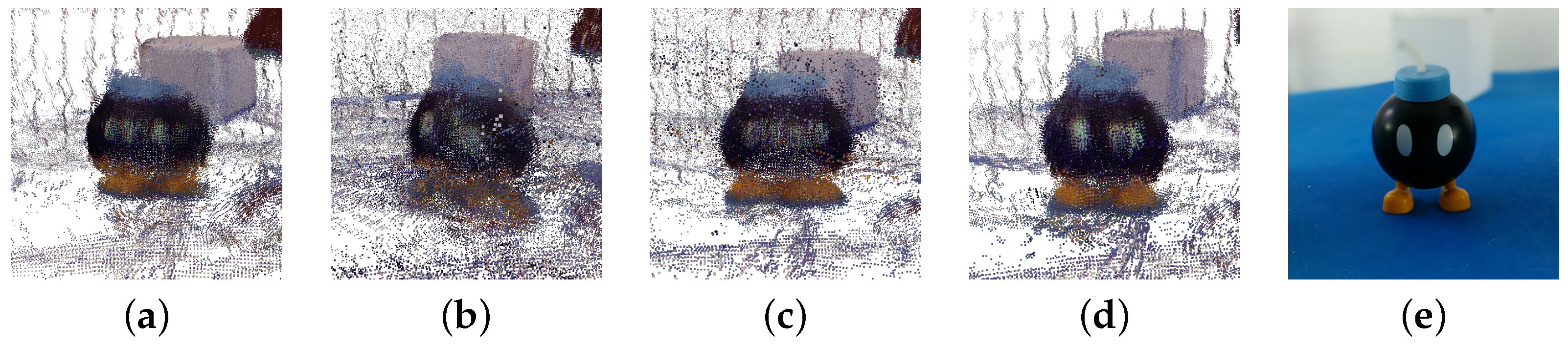
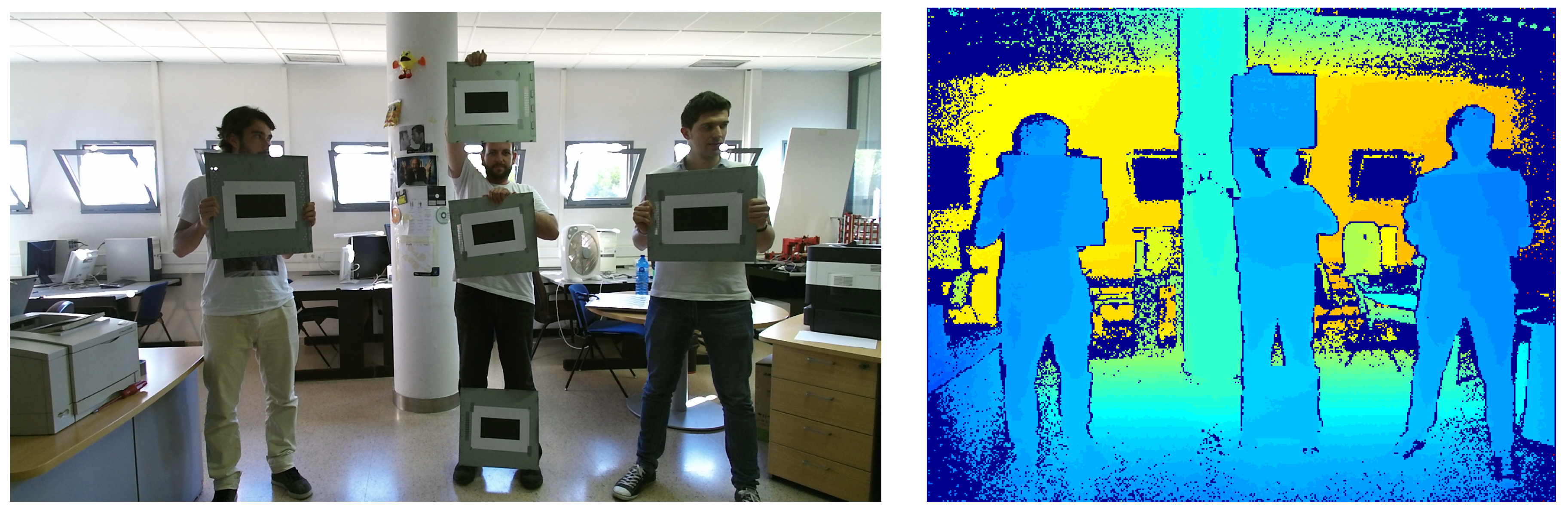
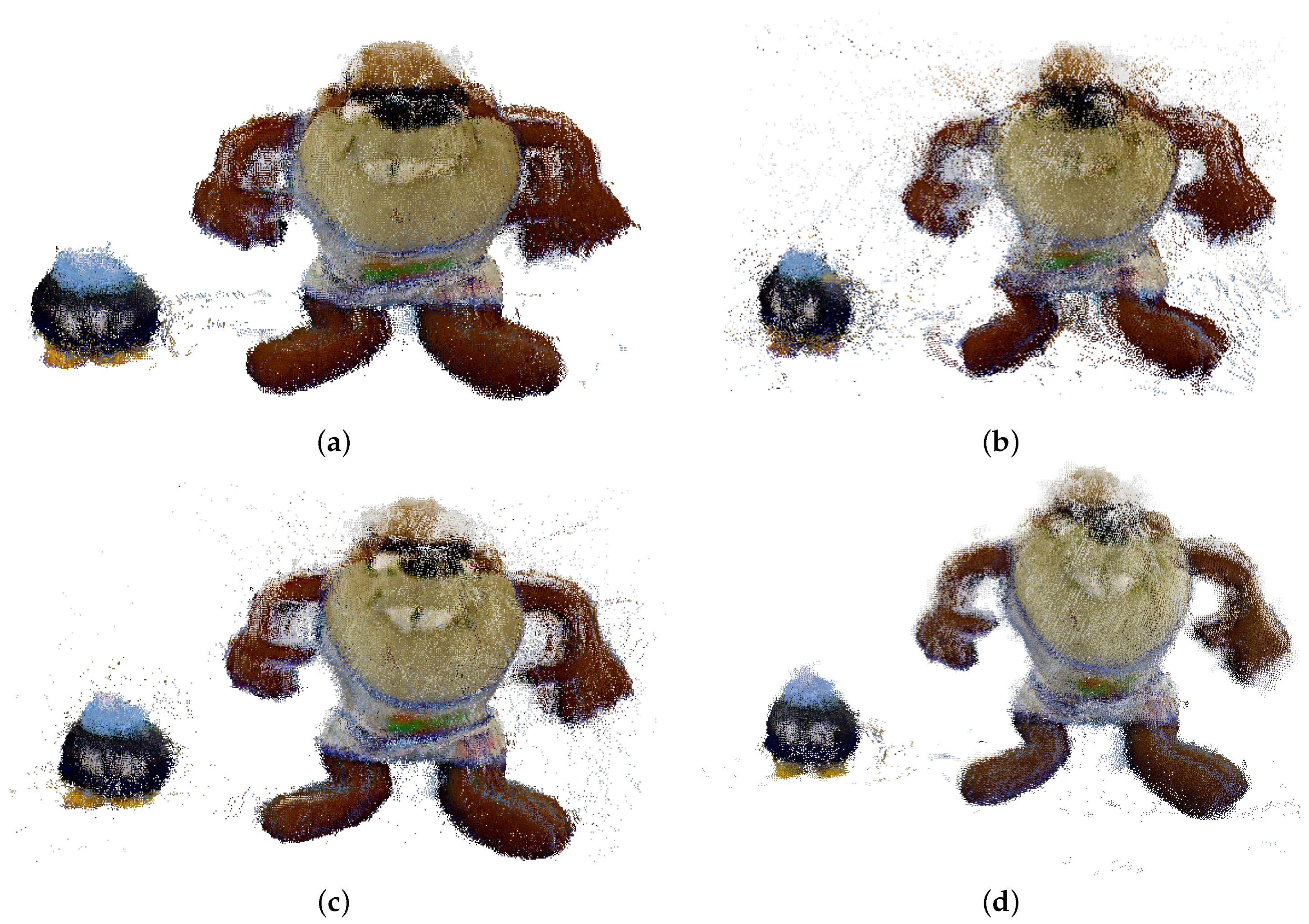
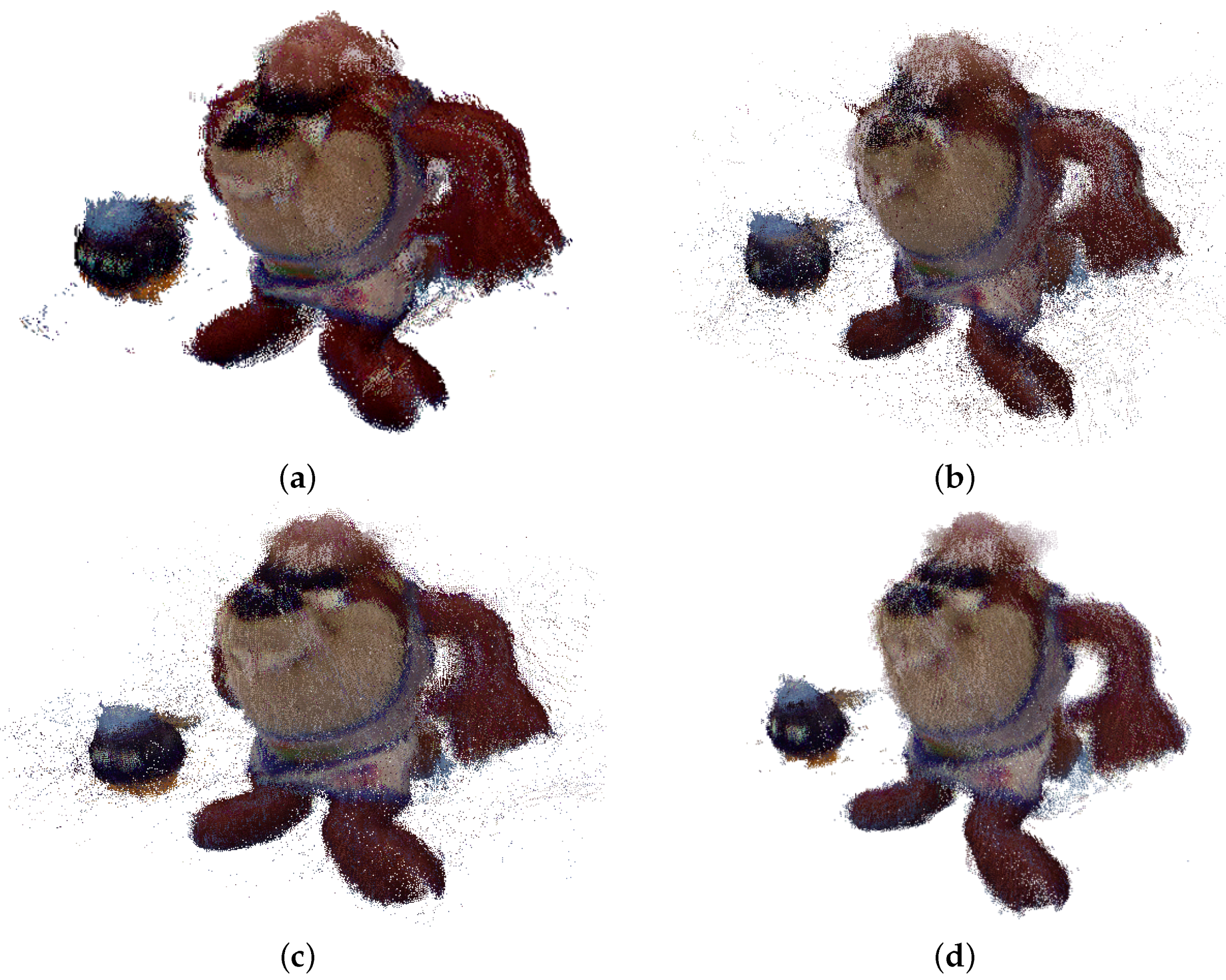
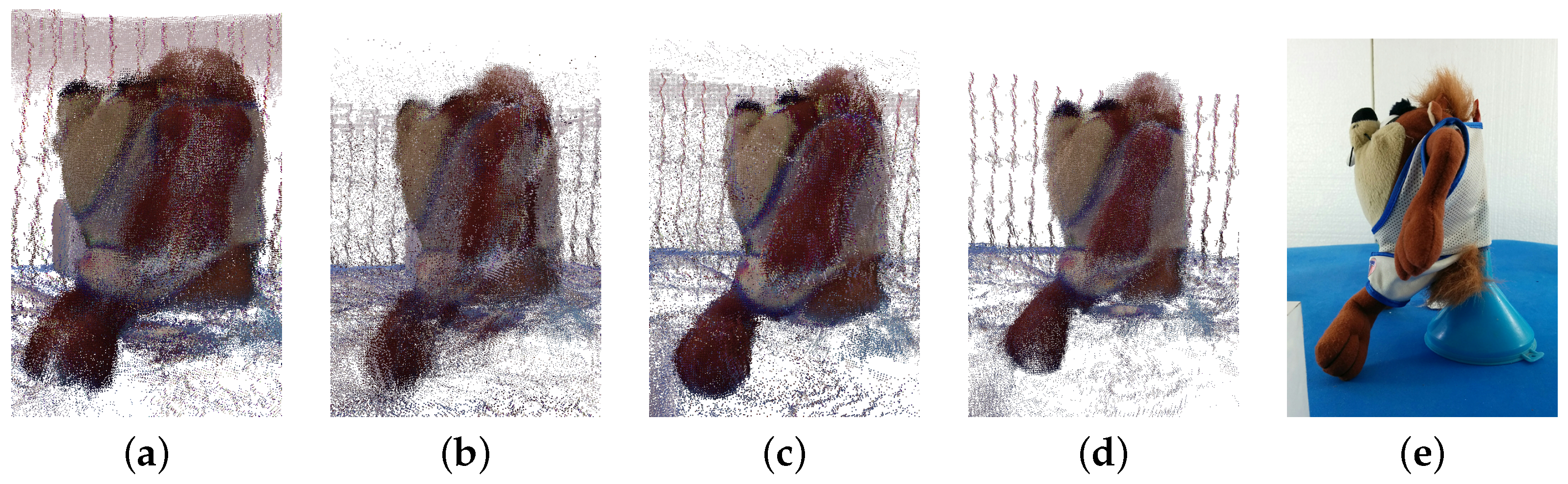
3.2.3. Object Registration
4. Conclusions
Author Contributions
Conflicts of Interest
Appendix A
Appendix A.1. Intrinsic Parameters
Appendix A.2. Extrinsic Parameters
References
- Saval-Calvo, M. Methodology Based on Registration Techniques for Representing Subjects and Their Deformations Acquired from General Purpose 3D Sensors. Ph.D. Thesis, University of Alicante, San Vicente del Raspeig, Spain, May 2015. [Google Scholar]
- Blais, F. Review of 20 years of range sensor development. J. Electron. Imaging 2004, 13, 231–240. [Google Scholar] [CrossRef]
- Chen, F.; Brown, G.M.; Song, M. Overview of three-dimensional shape measurement using optical methods. Opt. Eng. 2000, 39, 10–22. [Google Scholar]
- Besl, P.J. Active, optical range imaging sensors. Mach. Vis. Appl. 1988, 1, 127–152. [Google Scholar] [CrossRef]
- Sansoni, G.; Trebeschi, M.; Docchio, F. State-of-the-art and applications of 3D imaging sensors in industry, cultural heritage, medicine, and criminal investigation. Sensors 2009, 9, 568–601. [Google Scholar] [CrossRef] [PubMed]
- Davis, J.; Ramamoorthi, R.; Rusinkiewicz, S. Spacetime stereo: A unifying framework for depth from triangulation. In Proceedings of the 2003 IEEE Computer Society Conference on Computer Vision and Pattern Recognition, Madison, WI, USA, 18–20 June 2003; Volume 2, pp. II-359–II-366.
- Curless, B. Overview of active vision techniques. In Proceedings of the SIGGRAPH, 2000, Los Angesles, CA, USA, 9 August 1999; Volume 99.
- Poussart, D.; Laurendeau, D. 3-D sensing for industrial computer vision. In Advances in Machine Vision; Springer: New York, NY, USA, 1989; pp. 122–159. [Google Scholar]
- El-Hakim, S.F.; Beraldin, J.A.; Blais, F. Comparative evaluation of the performance of passive and active 3D vision systems. Proc. SPIE 1995, 2646, 14–25. [Google Scholar]
- Tippetts, B.; Lee, D.J.; Lillywhite, K.; Archibald, J. Review of stereo vision algorithms and their suitability for resource-limited systems. J. Real-Time Image Process. 2016, 11, 5–25. [Google Scholar] [CrossRef]
- Lazaros, N.; Sirakoulis, G.C.; Gasteratos, A. Review of Stereo Vision Algorithms: From Software to Hardware. Int. J. Optomech. 2008, 2, 435–462. [Google Scholar] [CrossRef]
- Kasper, A.; Xue, Z.; Dillmann, R. The KIT object models database: An object model database for object recognition, localization and manipulation in service robotics. Int. J. Robot. Res. 2012, 31, 927–934. [Google Scholar] [CrossRef]
- Lachat, E.; Macher, H.; Landes, T.; Grussenmeyer, P. Assessment and calibration of a RGB-D camera (Kinect v2 Sensor) towards a potential use for close-range 3D modeling. Remote Sens. 2015, 7, 13070–13097. [Google Scholar] [CrossRef]
- Chen, S.; Li, Y.; Wang, W.; Zhang, J. Active Sensor Planning for Multiview Vision Tasks; Springer: Heidelberg, Germany, 2008; Volume 1. [Google Scholar]
- Godin, G.; Beraldin, J.A.; Taylor, J.; Cournoyer, L.; Rioux, M.; El-Hakim, S.; Baribeau, R.; Blais, F.; Boulanger, P.; Domey, J.; et al. Active Optical 3D Imaging for Heritage Applications. IEEE Comput. Graph. Appl. 2002, 22, 24–36. [Google Scholar] [CrossRef]
- Foix, S.; Alenyà, G.; Torras, C. Lock-in time-of-flight (ToF) cameras: A survey. IEEE Sens. J. 2011, 11, 1917–1926. [Google Scholar] [CrossRef] [Green Version]
- Cui, Y.; Schuon, S.; Chan, D.; Thrun, S.; Theobalt, C. 3D shape scanning with a time-of-flight camera. In Proceedings of the IEEE Computer Society Conference on Computer Vision and Pattern Recognition, San Francisco, CA, USA, 13–18 June 2010; pp. 1173–1180.
- Horaud, R.; Hansard, M.; Evangelidis, G.; Clément, M. An Overview of Depth Cameras and Range Scanners Based on Time-of-Flight Technologies. Mach. Vis. Appl. J. 2016, 27, 1005–1020. [Google Scholar] [CrossRef] [Green Version]
- Lai, K.; Bo, L.; Ren, X.; Fox, D. Consumer Depth Cameras for Computer Vision. In Consumer Depth Cameras for Computer Vision; Springer: London, UK, 2013; p. 167. [Google Scholar]
- Khoshelham, K.; Elberink, S.O. Accuracy and resolution of Kinect depth data for indoor mapping applications. Sensors 2012, 12, 1437–1454. [Google Scholar] [CrossRef] [PubMed]
- Henry, P.; Krainin, M.; Herbst, E.; Ren, X.; Fox, D. RGB-D mapping: Using Kinect-style depth cameras for dense 3D modeling of indoor environments. Int. J. Robot. Res. 2012, 31, 647–663. [Google Scholar] [CrossRef]
- Meng, M.; Fallavollita, P.; Blum, T.; Eck, U.; Sandor, C.; Weidert, S.; Waschke, J.; Navab, N. Kinect for interactive AR anatomy learning. In Proceedings of the 2013 IEEE International Symposium on Mixed and Augmented Reality, ISMAR 2013, Adelaide, Australia, 1–4 October 2013; pp. 277–278.
- Zondervan, D.K.; Secoli, R.; Darling, A.M.; Farris, J.; Furumasu, J.; Reinkensmeyer, D.J. Design and Evaluation of the Kinect-Wheelchair Interface Controlled (KWIC) Smart Wheelchair for Pediatric Powered Mobility Training. Assist. Technol. 2015, 27, 183–192. [Google Scholar] [CrossRef] [PubMed]
- Han, J.; Shao, L.; Xu, D.; Shotton, J. Enhanced computer vision with Microsoft Kinect sensor: A review. IEEE Trans. Cybern. 2013, 43, 1318–1334. [Google Scholar] [PubMed]
- Shao, L.; Han, J.; Kohli, P.; Zhang, Z. Computer Vision and Machine Learning with RGB-D Sensors; Springer: Cham, Switzerland, 2014; p. 313. [Google Scholar]
- Morell-Gimenez, V.; Saval-Calvo, M.; Azorin-Lopez, J.; Garcia-Rodriguez, J.; Cazorla, M.; Orts-Escolano, S.; Fuster-Guillo, A. A comparative study of registration methods for RGB-D video of static scenes. Sensors 2014, 14, 8547–8576. [Google Scholar] [CrossRef] [PubMed]
- Weiss, A.; Hirshberg, D.; Black, M.J. Home 3D Body Scans from Noisy Image and Range Data. In Proceedings of the 2011 International Conference on Computer Vision, Barcelona, Spain, 6–13 November 2011; pp. 1951–1958.
- Lovato, C.; Bissolo, E.; Lanza, N.; Stella, A.; Giachetti, A. A Low Cost and Easy to Use Setup for Foot Scanning. In Proceedings of the 5th International Conference on 3D Body Scanning Technologies, Lugano, Switzerland, 21–22 October 2014; pp. 365–371.
- Jedvert, M. 3D Head Scanner. Master’s Thesis, Chalmers University of Technology, Göteborg, Sweden, 2013. [Google Scholar]
- Paier, W. Acquisition of 3D-Head-Models Using SLR-Cameras and RGBZ-Sensors. Master’s thesis, Freie Universität Berlin, Berlin, Germany, 2013. [Google Scholar]
- Smisek, J.; Jancosek, M.; Pajdla, T. 3D with Kinect. In Proceedings of the IEEE International Conference on Computer Vision, Barcelona, Spain, 6–13 November 2011; pp. 1154–1160.
- Herrera, C.D.; Kannala, J.; Heikkilä, J. Accurate and practical calibration of a depth and color camera pair. In Proceedings of the 14th International Conference on Computer Analysis of Images and Patterns, Seville, Spain, 29–31 August 2011; pp. 437–445.
- Zhang, C.; Zhang, Z. Calibration between depth and color sensors for commodity depth cameras. In Proceedings of the 2011 IEEE International Conference on Multimedia and Expo, Barcelona, Spain, 11–15 July 2011; pp. 1–6.
- Burrus, N. Kinect RGB Demo. Manctl Labs. Available online: http://rgbdemo.org/ (accessed on 21 January 2017).
- Daniel Herrera, C.; Kannala, J.; Heikkilä, J. Joint depth and color camera calibration with distortion correction. IEEE Trans. Pattern Anal. Mach. Intell. 2012, 34, 2058–2064. [Google Scholar] [CrossRef] [PubMed]
- Raposo, C.; Barreto, J.P.; Nunes, U. Fast and accurate calibration of a kinect sensor. In Proceedings of the 2013 International Conference on 3DTV-Conference, Seattle, WA, USA, 29 June–1 July 2013; pp. 342–349.
- Staranowicz, A.; Brown, G.R.; Morbidi, F.; Mariottini, G.L. Easy-to-use and accurate calibration of RGB-D cameras from spheres. In Proceedings of the 6th Pacific-Rim Symposium on Image and Video Technology, PSIVT 2013, Guanajuato, Mexico, 28 October–1 November 2013; pp. 265–278.
- Staranowicz, A.; Mariottini, G.L. A comparative study of calibration methods for Kinect-style cameras. In Proceedings of the 5th International Conference on PErvasive Technologies Related to Assistive Environments—PETRA ’12, Heraklion, Greece, 6–9 June 2012; ACM Press: New York, NY, USA, 2012; p. 1. [Google Scholar]
- Xiang, W.; Conly, C.; McMurrough, C.D.; Athitsos, V. A review and quantitative comparison of methods for kinect calibration. In Proceedings of the 2nd international Workshop on Sensor-Based Activity Recognition and Interaction—WOAR ’15, Rostock, Germany, 25–26 June 2015; ACM Press: New York, NY, USA, 2015; pp. 1–6. [Google Scholar]
- Teichman, A.; Miller, S.; Thrun, S. Unsupervised Intrinsic Calibration of Depth Sensors via SLAM. In Proceedings of the Robotics Science and Systems 2013, Berlin, Germany, 24–28 June 2013; Volume 248.
- Staranowicz, A.N.; Brown, G.R.; Morbidi, F.; Mariottini, G.L. Practical and accurate calibration of RGB-D cameras using spheres. Comput. Vis. Image Underst. 2015, 137, 102–114. [Google Scholar] [CrossRef]
- Salvi, J.; Pagès, J.; Batlle, J. Pattern codification strategies in structured light systems. Pattern Recognit. 2004, 37, 827–849. [Google Scholar] [CrossRef]
- Salvi, J.; Fernandez, S.; Pribanic, T.; Llado, X. A state of the art in structured light patterns for surface profilometry. Pattern Recognit. 2010, 43, 2666–2680. [Google Scholar] [CrossRef]
- Herakleous, K.; Poullis, C. 3DUNDERWORLD-SLS: An Open-Source Structured-Light Scanning System for Rapid Geometry Acquisition. arXiv, 2014; 1–30arXiv:1406.6595. [Google Scholar]
- Gupta, M.; Yin, Q.; Nayar, S.K. Structured light in sunlight. In Proceedings of the IEEE International Conference on Computer Vision, Sydney, Australia, 1–8 December 2013; pp. 545–552.
- Fuchs, S.; Hirzinger, G. Extrinsic and depth calibration of ToF-cameras. In Proceedings of the 26th IEEE Conference on Computer Vision and Pattern Recognition, CVPR, Anchorage, AK, USA, 23–28 June 2008.
- Freedman, B.; Shpunt, A.; Machline, M.; Arieli, Y. Depth Mapping Using Projected Patterns. U.S. Patent 8,493,496 B2, 23 July 2013. [Google Scholar]
- Zhang, Z. A flexible new technique for camera calibration. IEEE Trans. Pattern Anal. Mach. Intell. 2000, 22, 1330–1334. [Google Scholar] [CrossRef]
- Tsai, R.Y. A Versatile Camera Calibration Technique for High-Accuracy 3D Machine Vision Metrology Using Off-the-Shelf TV Cameras and Lenses. IEEE J. Robot. Autom. 1987, 3, 323–344. [Google Scholar] [CrossRef]
- Hartley, R.I.; Zisserman, A. Multiple View Geometry in Computer Vision, 2nd ed.; Cambridge University Press: Cambridge, UK, 2004. [Google Scholar]
- WolfWings File:Barrel distortion.svg. Available online: https://en.wikipedia.org/wiki/File:Barrel_distortion.svg (accessed on 22 January 2017).
- WolfWings File:Pincushion distortion.svg. Available online: https://en.wikipedia.org/wiki/File:Pincushion_distortion.svg (accessed on 22 January 2017).
- WolfWings File:Mustache distortion.svg. Available online: https://en.wikipedia.org/wiki/File:Mustache_distortion.svg (accessed on 22 January 2017).
- Schulze, M. An Approach for Calibration of a Combined RGB-Sensor and 3D Camera Device; Institute of Photogrammetry and Remote Sensing, Technische Universität Dresde: Dresden, Germany, 2011. [Google Scholar]
- Remondino, F.; Fraser, C. Digital camera calibration methods: Considerations and comparisons. Int. Arch. Photogramm. Remote Sens. Spat. Inf. Sci. 2006, 36, 266–272. [Google Scholar]
- Bouguet, J.Y. Camera Calibration Toolbox for Matlab. 2004. Available online: https://www.vision.caltech.edu/bouguetj/calib_doc/ (accessed on 22 December 2016).
- Daniel, H.C. Kinect Calibration Toolbox; Center for Machine Vision Research, University of Oulu: Oulu, Finland, 2012; Available online: http://www.ee.oulu.fi/~dherrera/kinect/ (accessed on 22 December 2016).
- Manuel Fernandez, E.L.; Lucas, T.; Marcelo, G. ANSI C Implementation of Classical Camera Calibration Algorithms: Tsai and Zhang. Available online: http://webserver2.tecgraf.puc-rio.br/~mgattass/calibration/ (accessed on 22 December 2016).
- Raposo, C.; Barreto, J.P.; Nunes, U. EasyKinCal. Available online: http://arthronav.isr.uc.pt/~carolina/kinectcalib/ (accessed on 22 December 2016).
- Staranowicz, A.; Brown, G.; Morbidi, F.; Mariottini, G. Easy-to-Use and Accurate Calibration of RGB-D Cameras from Spheres. Available online: http://ranger.uta.edu/~gianluca/research/assistiverobotics_rgbdcalibration.html (accessed on 22 December 2016).
- Lichti, D.D. Self-calibration of a 3D range camera. Archives 2008, 37, 1–6. [Google Scholar]
- Zhu, J.; Wang, L.; Yang, R.; Davis, J. Fusion of time-of-flight depth and stereo for high accuracy depth maps. In Proceedings of the 2008 IEEE Conference on Computer Vision and Pattern Recognition, Anchorage, AK, USA, 23–28 June 2008; pp. 1–8.
- Lindner, M.; Kolb, A. Lateral and Depth Calibration of PMD-Distance Sensors. In Advances in Visual Computing; Springer: Berlin/Heidelberg, Germany, 2006; pp. 524–533. [Google Scholar]
- Zhang, Z.Z.Z. Flexible camera calibration by viewing a plane from unknown orientations. In Proceedings of the Seventh IEEE International Conference on Computer Vision, Corfu, Greece, 20–27 September 1999; Volume 1, pp. 666–673.
- Van Den Bergh, M.; Van Gool, L. Combining RGB and ToF cameras for real-time 3D hand gesture interaction. In Proceedings of the 2011 IEEE Workshop on Applications of Computer Vision, WACV 2011, Kona, HI, USA, 5–7 January 2011; pp. 66–72.
- Hartley, R.I. Theory and Practice of Projective. Int. J. Comput. Vis. 1998, 35, 115–127. [Google Scholar] [CrossRef]
- Fischler, M.A.; Bolles, R.C. Random sample consensus: A paradigm for model fitting with applications to image analysis and automated cartography. Commun. ACM 1981, 24, 381–395. [Google Scholar] [CrossRef]
- Saval-Calvo, M.; Azorin-Lopez, J.; Fuster-Guillo, A.; Mora-Mora, H. μ-MAR: Multiplane 3D Marker based Registration for depth-sensing cameras. Expert Syst. Appl. 2015, 42, 9353–9365. [Google Scholar] [CrossRef]
- Bradski, G.; Kaehler, A. Learning OpenCV: Computer Vision with the OpenCV Library; O’Reilly Media, Inc.: Newton, MA, USA, 2008. [Google Scholar]
- Weng, J.; Coher, P.; Herniou, M. Camera Calibration with Distortion Models and Accuracy Evaluation. IEEE Trans. Pattern Anal. Mach. Intell. 1992, 14, 965–980. [Google Scholar] [CrossRef]


| Sensor | Measuring Range (m) | Error | Field of View HxV (Degrees) | Resolution Colour/Depth | Depth Resolution (cm) | Technology | FPS |
|---|---|---|---|---|---|---|---|
| Kinect v1 | 0.8–3.5 | <4 cm | 57 × 43 | 640 × 480 640 × 480 | 1 @ 2 m | SL | 15/30 |
| Carmine 1.08 | 0.8–3.5 | - | 57.5 × 45 | 640 × 480 640 × 480 | 1.2 @ 2 m | SL | 60 |
| Carmine 1.09 | 0.35–1.4 | - | 57.5 × 45 | 640 × 480 640 × 480 | 0.1 @ 0.5 m | SL | 60 |
| Xtion Pro | 0. 8–3. 5 | - | 58 × 45 | 1280 × 1024 640 × 480 | 1 @ 2 m | SL | 30/60 |
| Real Sense | 0. 2–1. 2 | 1% | 59 × 46 | 1920 × 1080 640 × 480 | - | SL | 30/60 |
| Kinect v2 | 0. 5–4. 5 | 0.5% | 70 × 60 | 1920 × 1080 512 × 424 | 2 @ 2 m | ToF | 15/30 |
| Senz3D | 0. 2–1. 0 | - | 74 × 41. 6 | 1080 × 720 320 × 240 | - | ToF | 30 |
| Method | Year | Citations | Joint Calibration | Input Data | Type of Target | Known Target | Number of Images (Approx.) | Available Code |
|---|---|---|---|---|---|---|---|---|
| Daniel Herrera et al. [35] | 2012 | 223 | Y | D,C | Chessboard | Y | 20 | Y [57] |
| Zhang and Zhang [33] | 2011 | 107 | Y | Z,C | Chessboard | Y | 12 | Y [58] |
| [34] | 2011 | 37 | Y | I,Z,C | Chessboard | Y | 30 | Y [34] |
| Bouguet [56] | 2004 | 2721 | N | I,C | Chessboard | Y | 20 | Y [56] |
| Raposo et al. [36] | 2013 | 30 | Y | D,C | Chessboard | Y | 10 | Y [59] |
| Staranowicz et al. [37] | 2014 | 13 | Y | Z,C | Spheres | N | - | Y [60] |
| Tsai [49] | 1987 | 7113 | N | C | Flat surface with squares | Y | 1–8 | Y [58] |
| Fuchs and Hirzinger [46] | 2008 | 150 | N | Z | Chessboard + robotic arm | Y | 50 | N |
| Lichti [61] | 2008 | 452 | N | Z | Rectangular targets of different sizes | N | - | N |
| Jiejie Zhu et al. [62] | 2008 | 251 | N | Z | Chessboard | Y | - | N |
| Lindner and Kolb [63] | 2007 | 76 | N | Z | Chessboard | Y | 68 | N |
| Burrus | Bouguet | Herrera | ||||
|---|---|---|---|---|---|---|
| RGB Camera | IR Camera | RGB Camera | IR Camera | RGB Camera | IR Camera | |
| 0 | ||||||
| 0 | ||||||
| 0 | 0 | 0 | ||||
| 0 | ||||||
| 0 | 0 | |||||
| − | − | − | − | − | ||
| − | − | − | − | − | ||
| − | − | − | − | − | ||
| − | − | − | − | − | ||
| R | ± | ± | ||||
| T | ± | ± | ||||
| Burrus | Bouguet | Herrera | ||||
|---|---|---|---|---|---|---|
| RGB Camera | IR Camera | RGB Camera | IR Camera | RGB Camera | IR Camera | |
| 307 | ||||||
| 0 | ||||||
| 0 | ||||||
| 0 | 0 | 0 | ||||
| 0 | ||||||
| 0 | ||||||
| − | − | − | − | − | ||
| − | − | − | − | − | ||
| − | − | − | − | − | ||
| − | − | − | − | − | ||
| R | ± | ± | ||||
| T | ± | ± | ||||
| Burrus | Bouguet | |||
|---|---|---|---|---|
| RGB Camera | IR Camera | RGB Camera | IR Camera | |
| 0 | 0 | |||
| R | ± | |||
| T | ± | |||
© 2017 by the authors. Licensee MDPI, Basel, Switzerland. This article is an open access article distributed under the terms and conditions of the Creative Commons Attribution (CC BY) license ( http://creativecommons.org/licenses/by/4.0/).
Share and Cite
Villena-Martínez, V.; Fuster-Guilló, A.; Azorín-López, J.; Saval-Calvo, M.; Mora-Pascual, J.; Garcia-Rodriguez, J.; Garcia-Garcia, A. A Quantitative Comparison of Calibration Methods for RGB-D Sensors Using Different Technologies. Sensors 2017, 17, 243. https://doi.org/10.3390/s17020243
Villena-Martínez V, Fuster-Guilló A, Azorín-López J, Saval-Calvo M, Mora-Pascual J, Garcia-Rodriguez J, Garcia-Garcia A. A Quantitative Comparison of Calibration Methods for RGB-D Sensors Using Different Technologies. Sensors. 2017; 17(2):243. https://doi.org/10.3390/s17020243
Chicago/Turabian StyleVillena-Martínez, Víctor, Andrés Fuster-Guilló, Jorge Azorín-López, Marcelo Saval-Calvo, Jeronimo Mora-Pascual, Jose Garcia-Rodriguez, and Alberto Garcia-Garcia. 2017. "A Quantitative Comparison of Calibration Methods for RGB-D Sensors Using Different Technologies" Sensors 17, no. 2: 243. https://doi.org/10.3390/s17020243