Earthquake Damage Visualization (EDV) Technique for the Rapid Detection of Earthquake-Induced Damages Using SAR Data


Abstract
:1. Introduction
2. Methodology
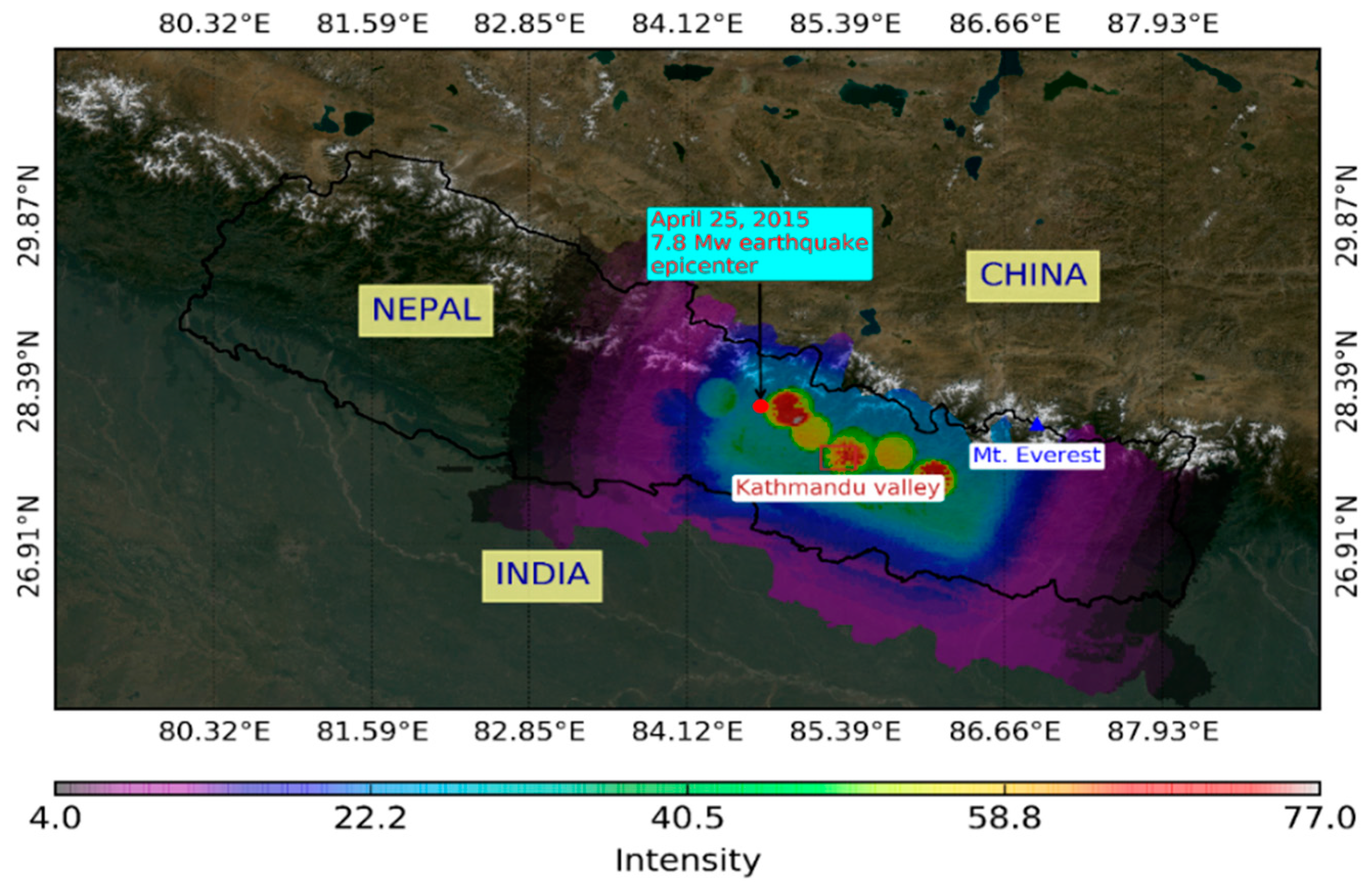
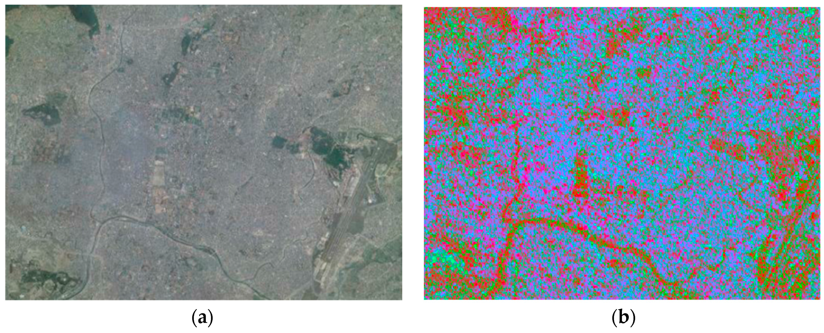
2.1. Study Area
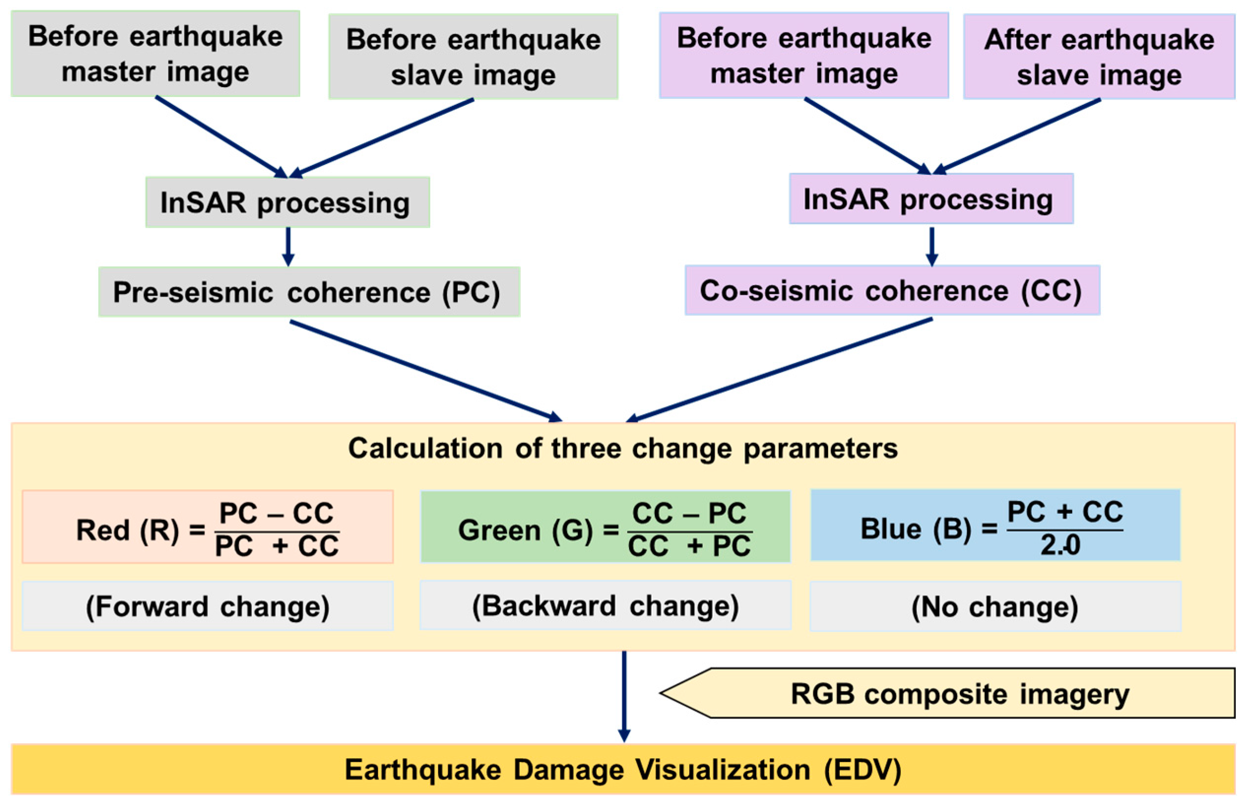
2.2. Proposal of the EDV
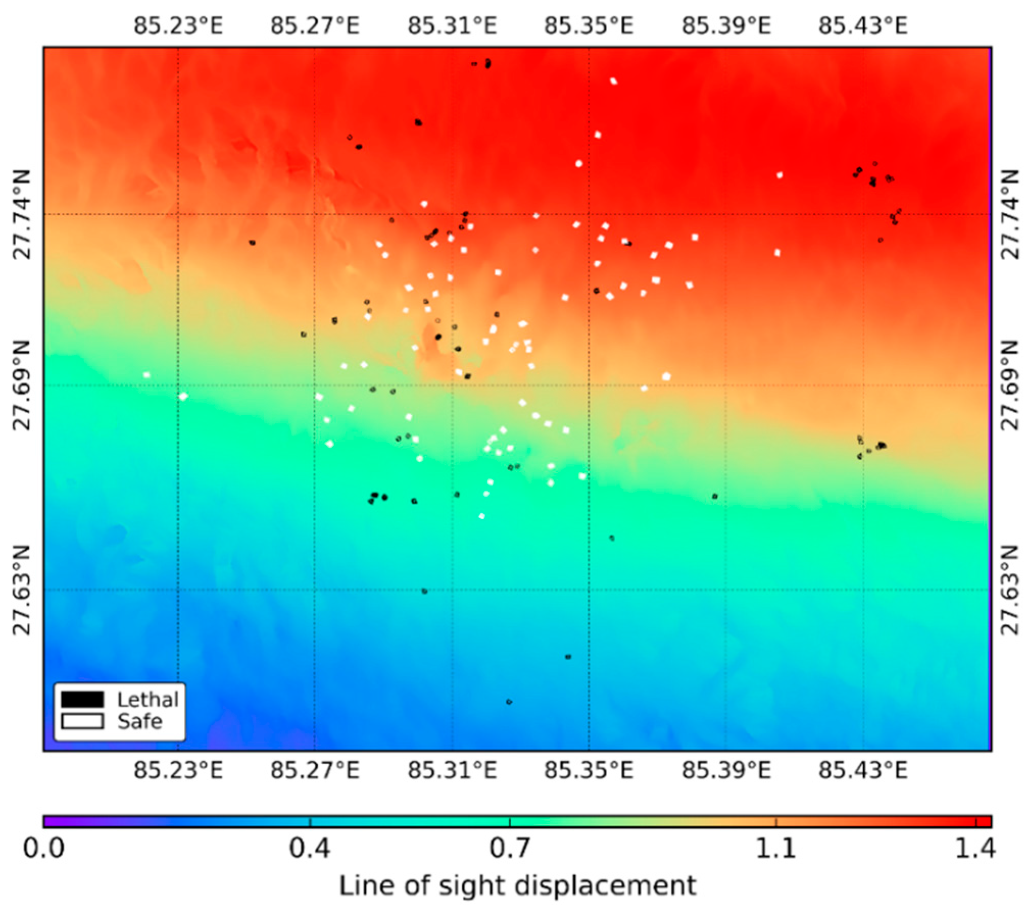
2.3. Validation Approach
3. Results and Discussion
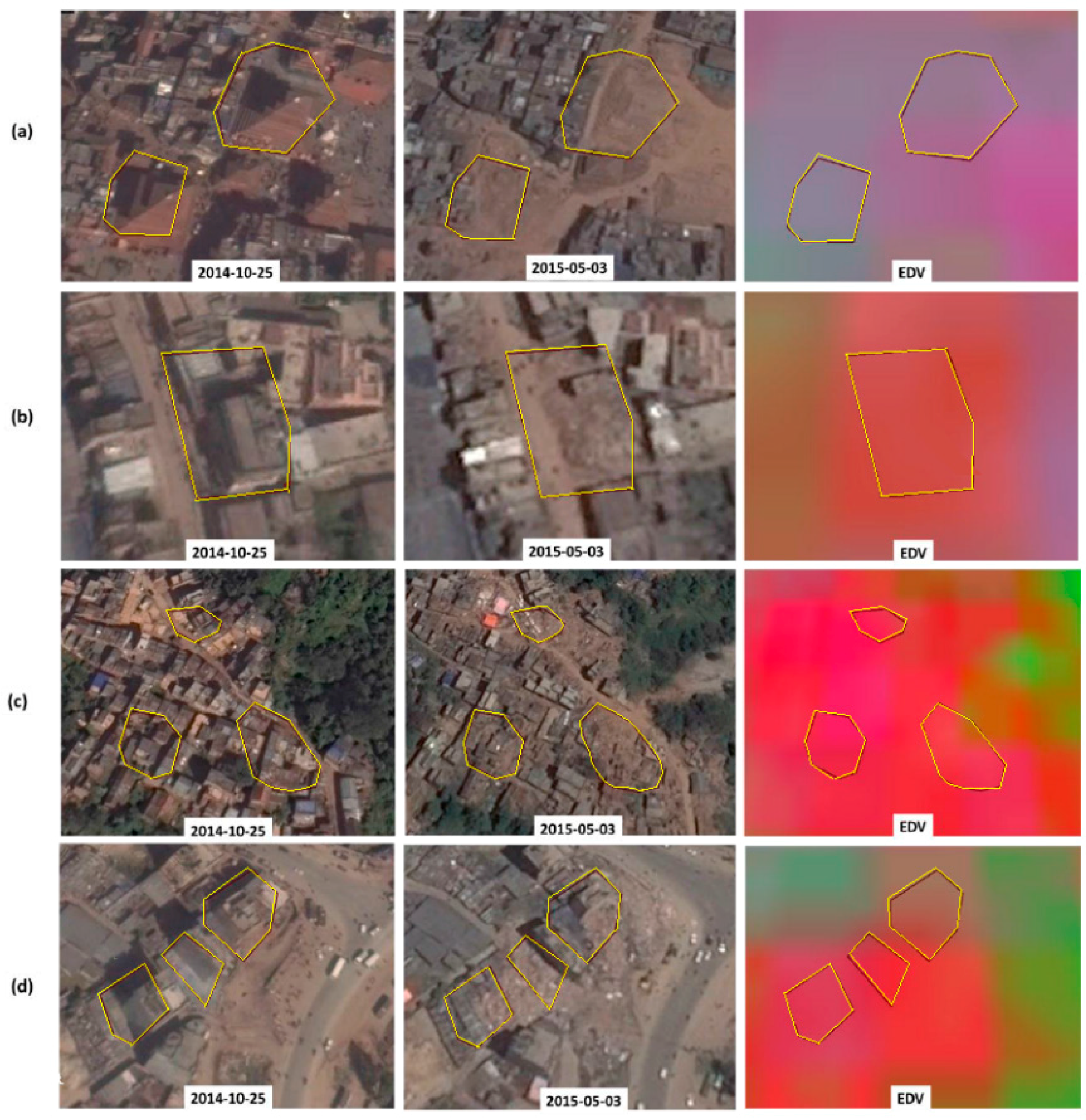
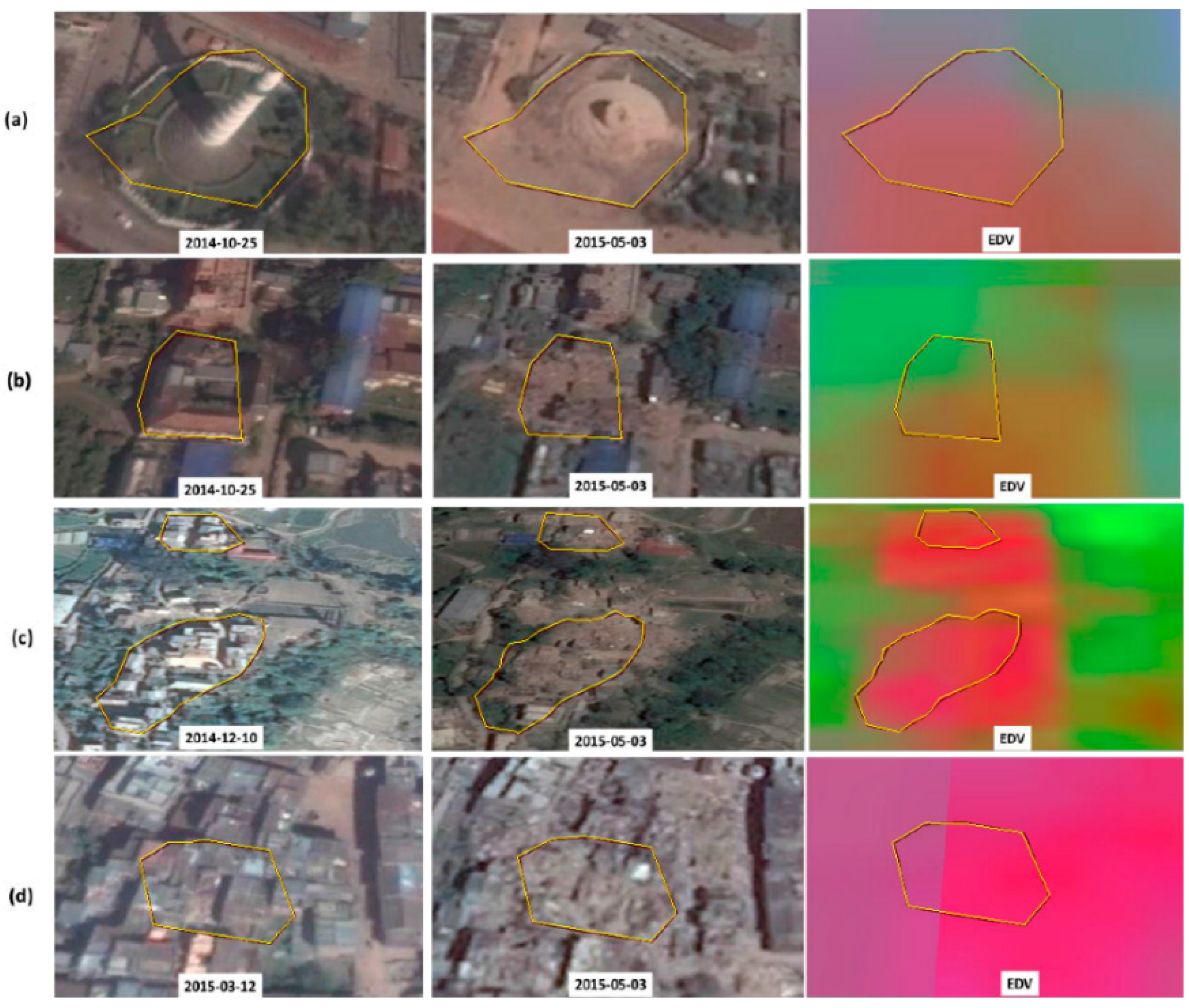
3.1. Performance of the EDV
3.2. Comparison to the NDPM
3.3. Cross-Validation Results
4. Conclusions
Acknowledgments
Author Contributions
Conflicts of Interest
References
- Dong, L.; Shan, J. A comprehensive review of earthquake-induced building damage detection with remote sensing techniques. ISPRS J. Photogramm. Remote Sens. 2013, 84, 85–99. [Google Scholar] [CrossRef]
- Matsuoka, M.; Yamazaki, F. Use of Satellite SAR Intensity Imagery for Detecting Building Areas Damaged Due to Earthquakes. Earthq. Spectra 2004, 20, 975–994. [Google Scholar] [CrossRef]
- Turker, M.; San, B.T. SPOT HRV data analysis for detecting earthquake-induced changes in Izmit, Turkey. Int. J. Remote Sens. 2003, 24, 2439–2450. [Google Scholar] [CrossRef]
- Yusuf, Y.; Matsuoka, M.; Yamazaki, F. Damage assessment after 2001 Gujarat earthquake using Landsat-7 satellite images. J. Indian Soc. Remote Sens. 2001, 29, 17–22. [Google Scholar] [CrossRef]
- Saito, K.; Spence, R.J.S.; Going, C.; Markus, M. Using High-Resolution Satellite Images for Post-Earthquake Building Damage Assessment: A Study Following the 26 January 2001 Gujarat Earthquake. Earthq. Spectra 2004, 20, 145–169. [Google Scholar] [CrossRef]
- Arciniegas, G.A.; Bijker, W.; Kerle, N.; Tolpekin, V.A. Coherence- and Amplitude-Based Analysis of Seismogenic Damage in Bam, Iran, Using Envisat ASAR Data. IEEE Trans. Geosci. Remote Sens. 2007, 45, 1571–1581. [Google Scholar] [CrossRef]
- Gamba, P.; Dell’Acqua, F.; Trianni, G. Rapid Damage Detection in the Bam Area Using Multitemporal SAR and Exploiting Ancillary Data. IEEE Trans. Geosci. Remote Sens. 2007, 45, 1582–1589. [Google Scholar] [CrossRef]
- Hoffmann, J. Mapping damage during the Bam (Iran) earthquake using interferometric coherence. Int. J. Remote Sens. 2007, 28, 1199–1216. [Google Scholar] [CrossRef]
- Chini, M.; Pierdicca, N.; Emery, W.J. Exploiting SAR and VHR Optical Images to Quantify Damage Caused by the 2003 Bam Earthquake. IEEE Trans. Geosci. Remote Sens. 2009, 47, 145–152. [Google Scholar] [CrossRef]
- Chini, M.; Cinti, F.R.; Stramondo, S. Co-seismic surface effects from very high resolution panchromatic images: the case of the 2005 Kashmir (Pakistan) earthquake. Nat. Hazards Earth Syst. Sci. 2011, 11, 931–943. [Google Scholar] [CrossRef] [Green Version]
- Miura, H.; Midorikawa, S.; Kerle, N. Detection of Building Damage Areas of the 2006 Central Java, Indonesia, Earthquake through Digital Analysis of Optical Satellite Images. Earthq. Spectra 2013, 29, 453–473. [Google Scholar] [CrossRef]
- Ehrlich, D.; Guo, H.D.; Molch, K.; Ma, J.W.; Pesaresi, M. Identifying damage caused by the 2008 Wenchuan earthquake from VHR remote sensing data. Int. J. Digit. Earth 2009, 2, 309–326. [Google Scholar] [CrossRef]
- Balz, T.; Liao, M. Building-damage detection using post-seismic high-resolution SAR satellite data. Int. J. Remote Sens. 2010, 31, 3369–3391. [Google Scholar] [CrossRef]
- Brunner, D.; Lemoine, G.; Bruzzone, L. Earthquake Damage Assessment of Buildings Using VHR Optical and SAR Imagery. IEEE Trans. Geosci. Remote Sens. 2010, 48, 2403–2420. [Google Scholar] [CrossRef]
- Pan, G.; Tang, D. Damage information derived from multi-sensor data of the Wenchuan Earthquake of May 2008. Int. J. Remote Sens. 2010, 31, 3509–3519. [Google Scholar] [CrossRef]
- Dell’Acqua, F.; Bignami, C.; Chini, M.; Lisini, G.; Polli, D.A.; Stramondo, S. Earthquake Damages Rapid Mapping by Satellite Remote Sensing Data: L’Aquila April 6th, 2009 Event. IEEE J. Sel. Top. Appl. Earth Obs. Remote Sens. 2011, 4, 935–943. [Google Scholar] [CrossRef]
- Corbane, C.; Saito, K.; Dell’Oro, L.; Bjorgo, E.; Gill, S.P.D.; Emmanuel Piard, B.; Huyck, C.K.; Kemper, T.; Lemoine, G.; Spence, R.J.S.; et al. A Comprehensive Analysis of Building Damage in the 12 January 2010 Mw7 Haiti Earthquake Using High-Resolution Satelliteand Aerial Imagery. Photogramm. Eng. Remote Sens. 2011, 77, 997–1009. [Google Scholar] [CrossRef]
- Tian, J.; Nielsen, A.A.; Reinartz, P. Building damage assessment after the earthquake in Haiti using two post-event satellite stereo imagery and DSMs. Int. J. Image Data Fusion 2015, 6, 155–169. [Google Scholar] [CrossRef] [Green Version]
- Miura, H.; Midorikawa, S.; Matsuoka, M. Building Damage Assessment Using High-Resolution Satellite SAR Images of the 2010 Haiti Earthquake. Earthq. Spectra 2016, 32, 591–610. [Google Scholar] [CrossRef]
- Hill, M.; Rossetto, T. Comparison of building damage scales and damage descriptions for use in earthquake loss modelling in Europe. Bull. Earthq. Eng. 2008, 6, 335–365. [Google Scholar] [CrossRef]
- Dolce, M.; Goretti, A. Building damage assessment after the 2009 Abruzzi earthquake. Bull. Earthq. Eng. 2015, 13, 2241–2264. [Google Scholar] [CrossRef]
- Schwarz, J.; Abrahamczyk, L.; Leipold, M.; Wenk, T. Vulnerability assessment and damage description for RC frame structures following the EMS-98 principles. Bull. Earthq. Eng. 2015, 13, 1141–1159. [Google Scholar] [CrossRef]
- Yamazaki, F.; Yano, Y.; Matsuoka, M. Visual Damage Interpretation of Buildings in Bam City Using QuickBird Images Following the 2003 Bam, Iran, Earthquake. Earthq. Spectra 2005, 21, 329–336. [Google Scholar] [CrossRef]
- Kerle, N. Satellite-based damage mapping following the 2006 Indonesia earthquake—How accurate was it? Int. J. Appl. Earth Obs. Geoinform. 2010, 12, 466–476. [Google Scholar] [CrossRef]
- Ge, L.; Ng, A.H.-M.; Li, X.; Liu, Y.; Du, Z.; Liu, Q. Near real-time satellite mapping of the 2015 Gorkha earthquake, Nepal. Ann. GIS 2015, 21, 175–190. [Google Scholar] [CrossRef]
- Meslem, A.; Yamazaki, F.; Maruyama, Y. Accurate evaluation of building damage in the 2003 Boumerdes, Algeria earthquake from Quickbird satellite images. J. Earthq. Tsunami 2011, 5, 1–18. [Google Scholar] [CrossRef]
- Tong, X.; Hong, Z.; Liu, S.; Zhang, X.; Xie, H.; Li, Z.; Yang, S.; Wang, W.; Bao, F. Building-damage detection using pre- and post-seismic high-resolution satellite stereo imagery: A case study of the May 2008 Wenchuan earthquake. ISPRS J. Photogramm. Remote Sens. 2012, 68, 13–27. [Google Scholar] [CrossRef]
- Conners, R.W.; Trivedi, M.M.; Harlow, C.A. Segmentation of a high-resolution urban scene using texture operators. Comput. Vis. Graphics Image Process. 1984, 25, 273–310. [Google Scholar] [CrossRef]
- Gusella, L.; Adams, B.J.; Bitelli, G.; Huyck, C.K.; Mognol, A. Object-Oriented Image Understanding and Post-Earthquake Damage Assessment for the 2003 Bam, Iran, Earthquake. Earthq. Spectra 2005, 21, 225–238. [Google Scholar] [CrossRef]
- Tiede, D.; Lang, S.; Füreder, P.; Hölbling, D.; Hoffmann, C.; Zeil, P. Automated Damage Indication for Rapid Geospatial Reporting. Photogramm. Eng. Remote Sens. 2011, 77, 933–942. [Google Scholar] [CrossRef]
- Parape, C.; Premachandra, C.; Tamura, M. Optimization of structure elements for morphological hit-or-miss transform for building extraction from VHR airborne imagery in natural hazard areas. Int. J. Mach. Learn. Cyber. 2015, 6, 641–650. [Google Scholar] [CrossRef]
- Li, P.; Xu, H.; Guo, J. Urban building damage detection from very high resolution imagery using OCSVM and spatial features. Int. J. Remote Sens. 2010, 31, 3393–3409. [Google Scholar] [CrossRef]
- Vetrivel, A.; Gerke, M.; Kerle, N.; Vosselman, G. Identification of damage in buildings based on gaps in 3D point clouds from very high resolution oblique airborne images. ISPRS J. Photogramm. Remote Sens. 2015, 105, 61–78. [Google Scholar] [CrossRef]
- Taskin, G.; Ersoy, O.K.; Kamasak, M.E. Earthquake-induced damage classification from postearthquake satellite image using spectral and spatial features with support vector selection and adaptation. J. Appl. Remote Sens. 2015, 9, 096017. [Google Scholar] [CrossRef]
- Turker, M.; Cetinkaya, B. Automatic detection of earthquake-damaged buildings using DEMs created from pre- and post-earthquake stereo aerial photographs. Int. J. Remote Sens. 2005, 26, 823–832. [Google Scholar] [CrossRef]
- Gerke, M.; Kerle, N. Automatic Structural Seismic Damage Assessment with Airborne Oblique Pictometry© Imagery. Photogramm. Eng. Remote Sens. 2011, 77, 885–898. [Google Scholar] [CrossRef]
- Maruyama, Y.; Tashiro, A.; Yamazaki, F. Detection of collapsed buildings due to earthquakes using a digital surface model constructed from aerial images. J. Earthq. Tsunami 2014, 8, 1450003. [Google Scholar] [CrossRef]
- Cao, C.; Liu, D.; Singh, R.P.; Zheng, S.; Tian, R.; Tian, H. Integrated detection and analysis of earthquake disaster information using airborne data. Geomat. Nat. Hazards Risk 2016, 7, 1099–1128. [Google Scholar] [CrossRef]
- Hong, Z.; Tong, X.; Cao, W.; Jiang, S.; Chen, P.; Liu, S. Rapid three-dimensional detection approach for building damage due to earthquakes by the use of parallel processing of unmanned aerial vehicle imagery. J. Appl. Remote Sens. 2015, 9, 097292. [Google Scholar] [CrossRef]
- Fernandez Galarreta, J.; Kerle, N.; Gerke, M. UAV-based urban structural damage assessment using object-based image analysis and semantic reasoning. Nat. Hazards Earth Syst. Sci. 2015, 15, 1087–1101. [Google Scholar] [CrossRef]
- Stramondo, S.; Bignami, C.; Chini, M.; Pierdicca, N.; Tertulliani, A. Satellite radar and optical remote sensing for earthquake damage detection: Results from different case studies. Int. J. Remote Sens. 2006, 27, 4433–4447. [Google Scholar] [CrossRef]
- Bazi, Y.; Bruzzone, L.; Melgani, F. An unsupervised approach based on the generalized Gaussian model to automatic change detection in multitemporal SAR images. IEEE Trans. Geosci. Remote Sens. 2005, 43, 874–887. [Google Scholar] [CrossRef]
- Dong, Y.; Li, Q.; Dou, A.; Wang, X. Extracting damage caused by the 2008 Ms 8.0 Wenchuan earthquake from SAR remote sensing data. J. Asian Earth Sci. 2011, 40, 907–914. [Google Scholar] [CrossRef]
- Trianni, G.; Gamba, P. Damage detection from SAR imagery: Application to the 2003 Algeria and 2007 Peru earthquakes. Int. J. Navig. Obs. 2008, 2008, 762378. [Google Scholar] [CrossRef]
- Yun, S.-H.; Hudnut, K.; Owen, S.; Webb, F.; Simons, M.; Sacco, P.; Gurrola, E.; Manipon, G.; Liang, C.; Fielding, E.; et al. Rapid Damage Mapping for the 2015 Mw 7.8 Gorkha Earthquake Using Synthetic Aperture Radar Data from COSMO–SkyMed and ALOS-2 Satellites. Seismol. Res. Lett. 2015, 86, 1549–1556. [Google Scholar] [CrossRef]
- Grünthal, G. European Macroseismic Scale 1998: EMS-98; Imprimerie Joseph Beffort: Helfent-Bertrange, Luxembourg, 1998. [Google Scholar]


| Methods | k-Nearest Neighbors | Gaussian Naïve Bayes | Random Forests | Support Vector Machine |
|---|---|---|---|---|
| EDV | 0.82 (0.64) | 0.86 (0.71) | 0.76 (0.52) | 0.69 (0.38) |
| NDPM | 0.60 (0.20) | 0.71 (0.41) | 0.61 (0.21) | 0.59 (0.17) |
© 2017 by the authors. Licensee MDPI, Basel, Switzerland. This article is an open access article distributed under the terms and conditions of the Creative Commons Attribution (CC BY) license ( http://creativecommons.org/licenses/by/4.0/).
Share and Cite
Sharma, R.C.; Tateishi, R.; Hara, K.; Nguyen, H.T.; Gharechelou, S.; Nguyen, L.V. Earthquake Damage Visualization (EDV) Technique for the Rapid Detection of Earthquake-Induced Damages Using SAR Data. Sensors 2017, 17, 235. https://doi.org/10.3390/s17020235
Sharma RC, Tateishi R, Hara K, Nguyen HT, Gharechelou S, Nguyen LV. Earthquake Damage Visualization (EDV) Technique for the Rapid Detection of Earthquake-Induced Damages Using SAR Data. Sensors. 2017; 17(2):235. https://doi.org/10.3390/s17020235
Chicago/Turabian StyleSharma, Ram C., Ryutaro Tateishi, Keitarou Hara, Hoan Thanh Nguyen, Saeid Gharechelou, and Luong Viet Nguyen. 2017. "Earthquake Damage Visualization (EDV) Technique for the Rapid Detection of Earthquake-Induced Damages Using SAR Data" Sensors 17, no. 2: 235. https://doi.org/10.3390/s17020235