Adaptive Spatial Filter Based on Similarity Indices to Preserve the Neural Information on EEG Signals during On-Line Processing

 , , , ,
Abstract
:1. Introduction
2. Materials and Methods
2.1. Proposed Spatial Filter
2.1.1. Background on Spatial Filters LAR and WAR
2.1.2. Adaptive Spatial Filter
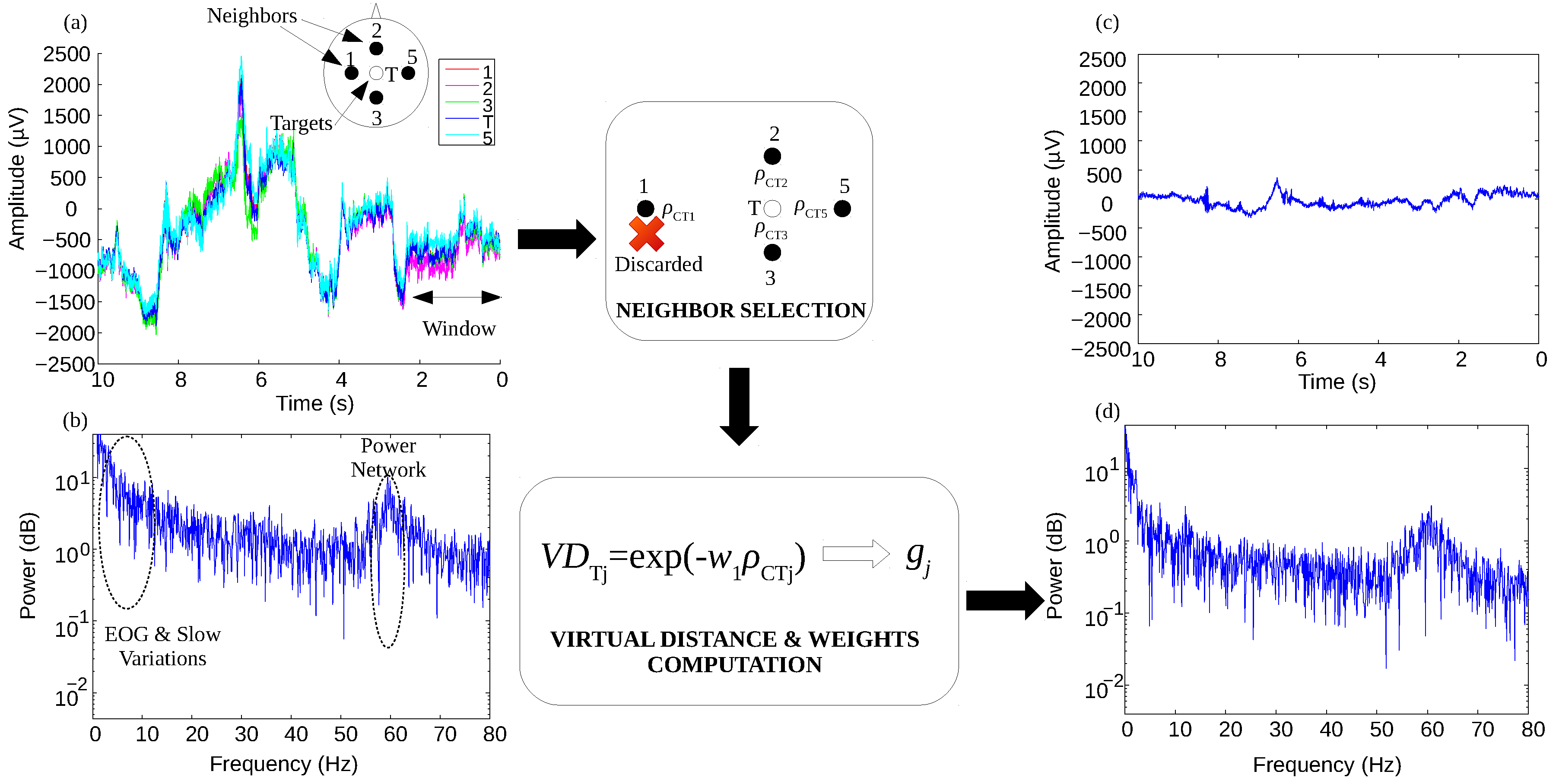
Neighbor Selection
Virtual Distance and Weights Computation
2.2. Statistical Analysis
2.2.1. Model Fitting and Optimization
2.2.2. SSVEP Database
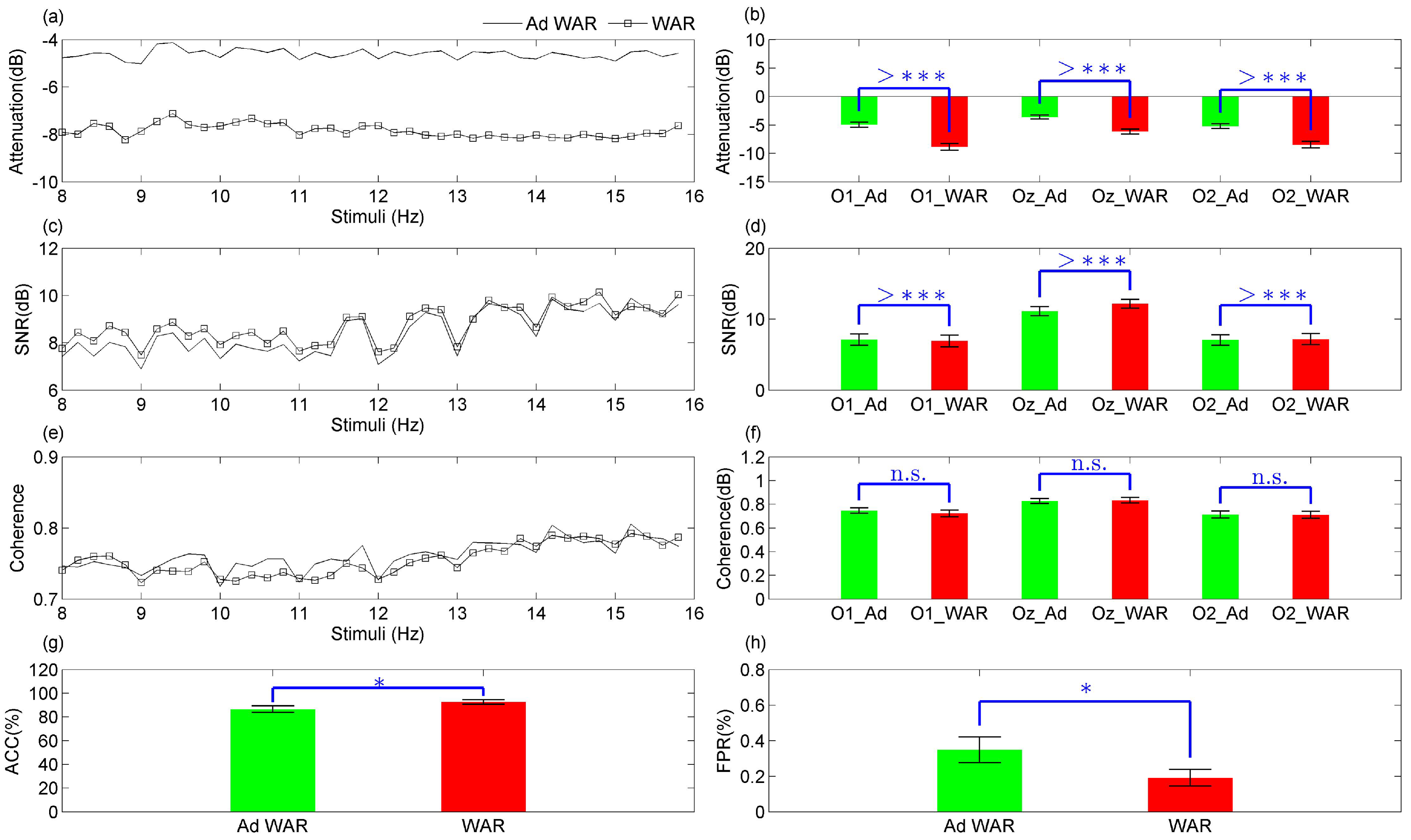
2.2.3. Preservation of SSVEP Components
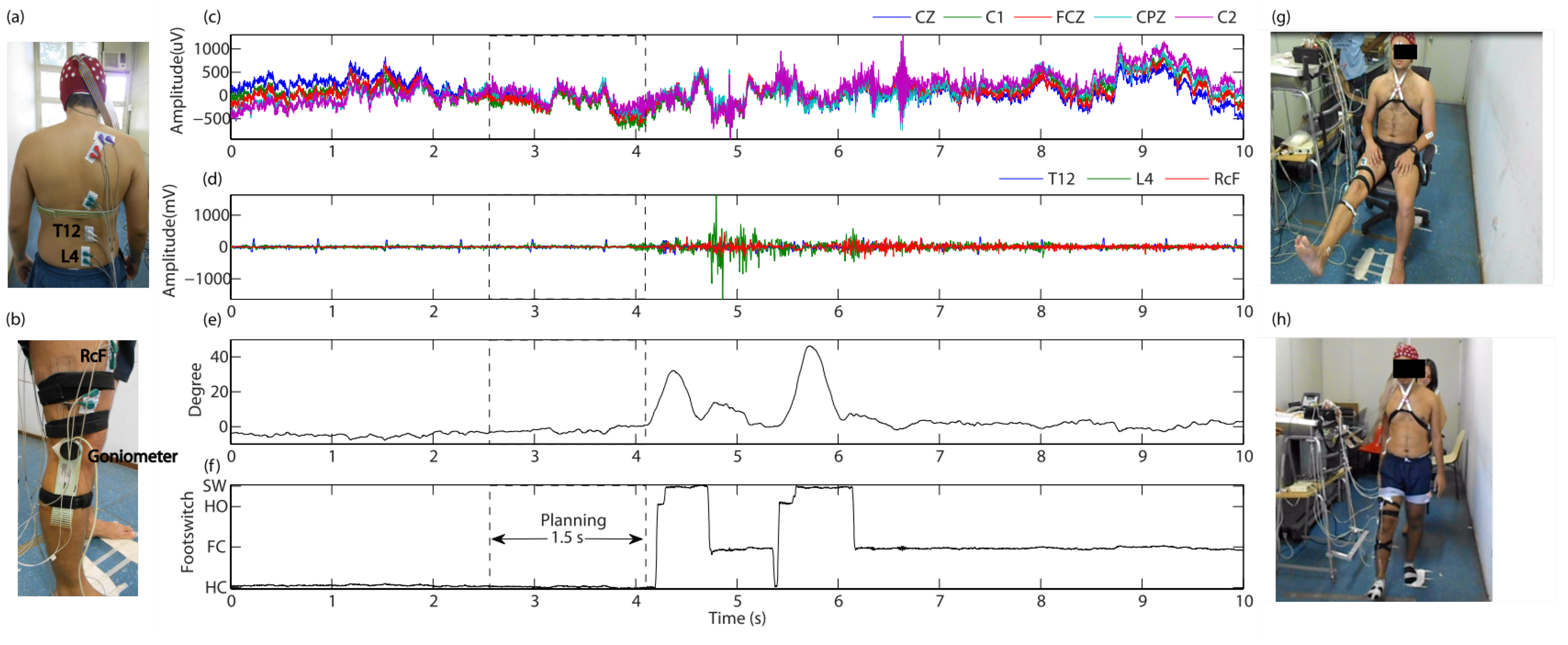
2.2.4. Application in a BCI for Gait Planning Recognition
Feature Extraction
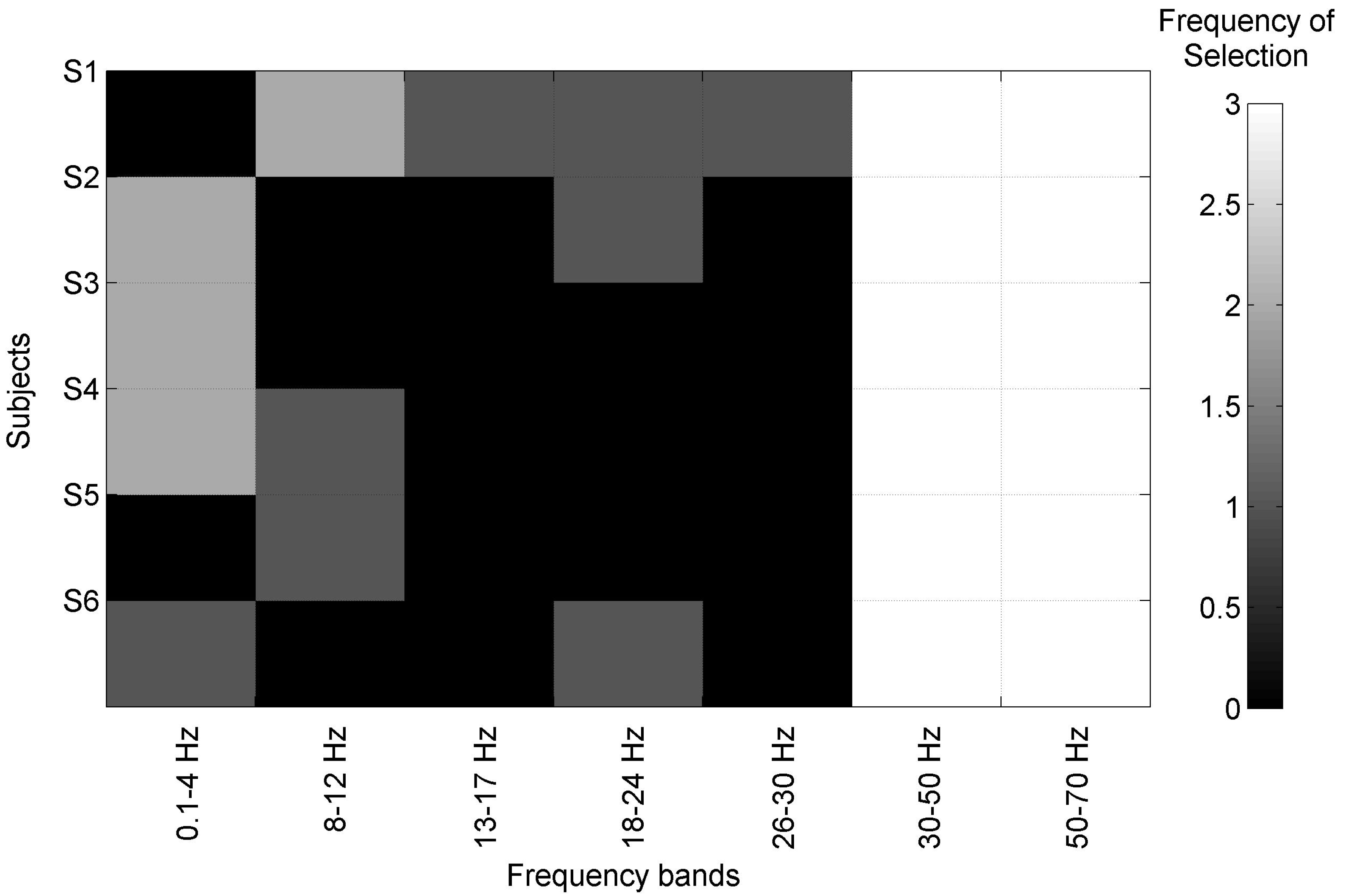
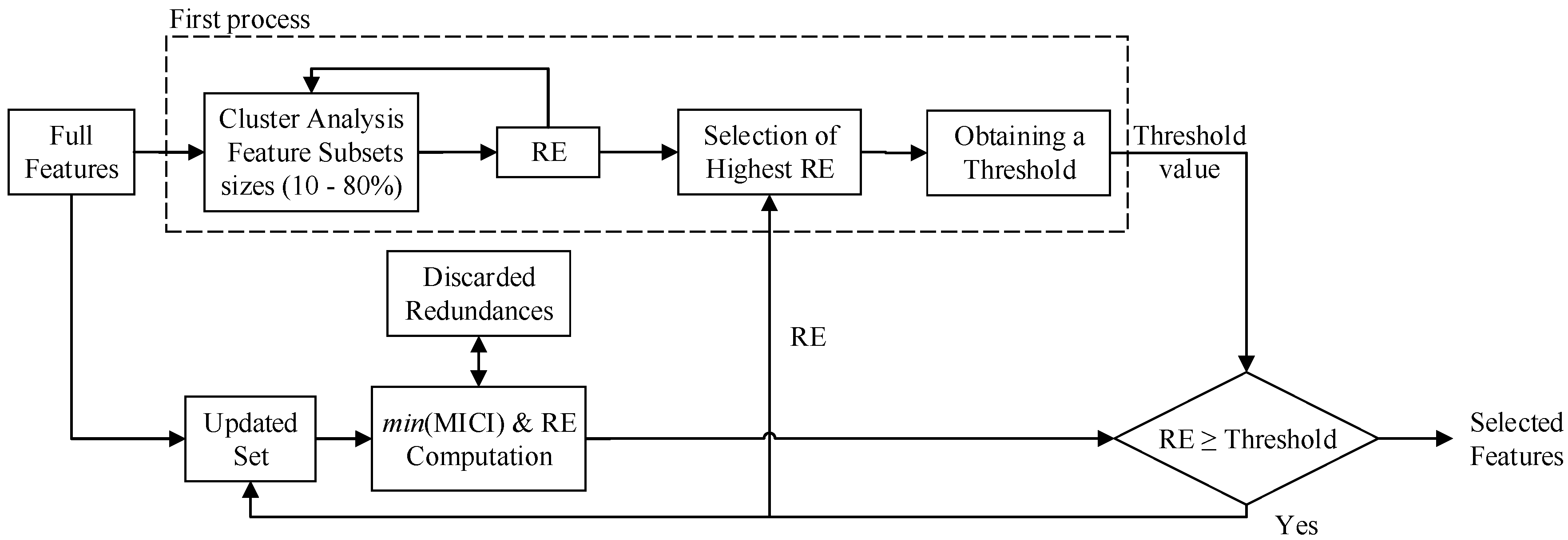
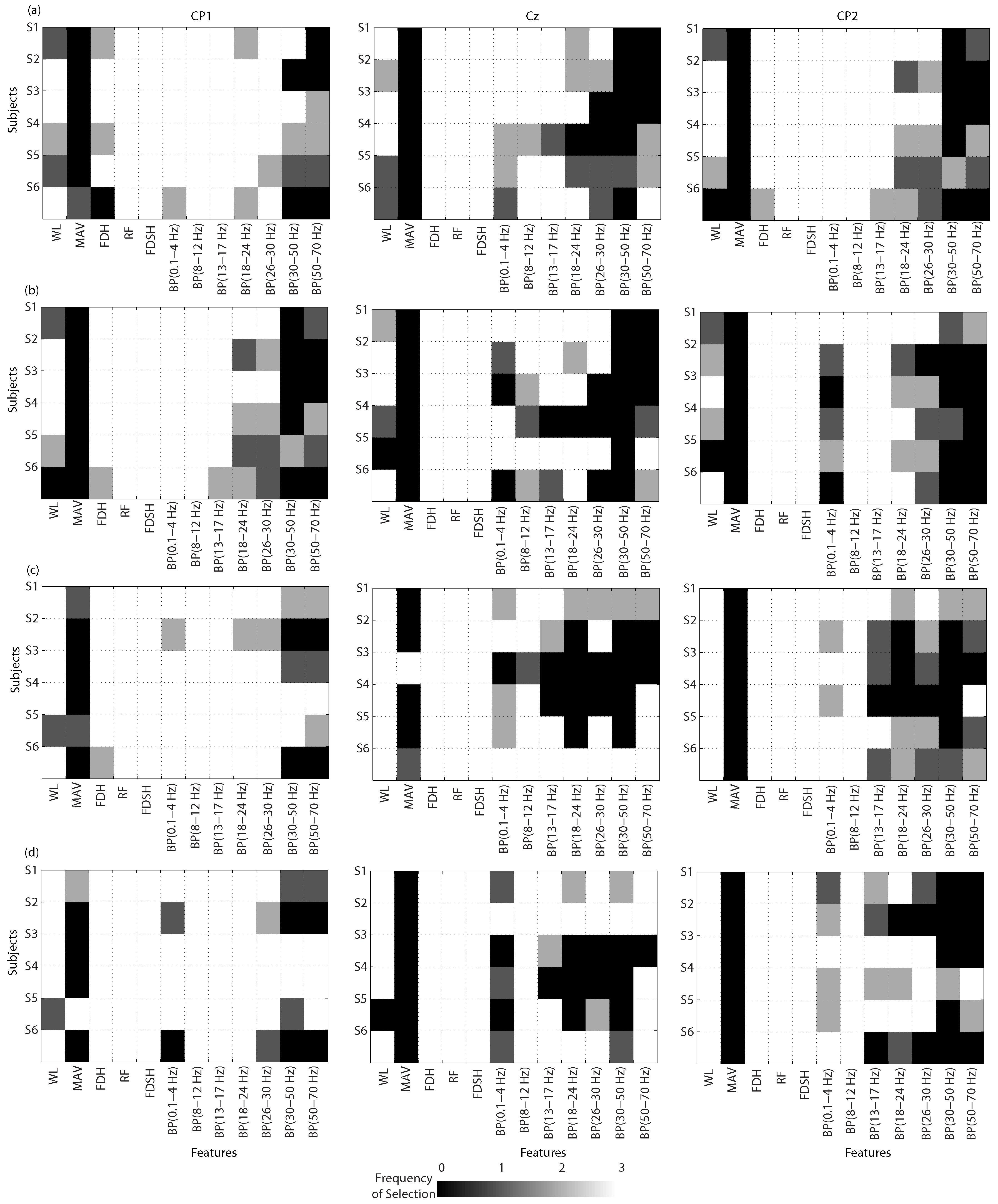
Feature Selection
Classification: Training Stage
BCI Validation
2.2.5. Protocol for Gait Planning Recognition
3. Results
3.1. Model Fitting Based on SSVEP
Analysis of SSVEP Components Preservation
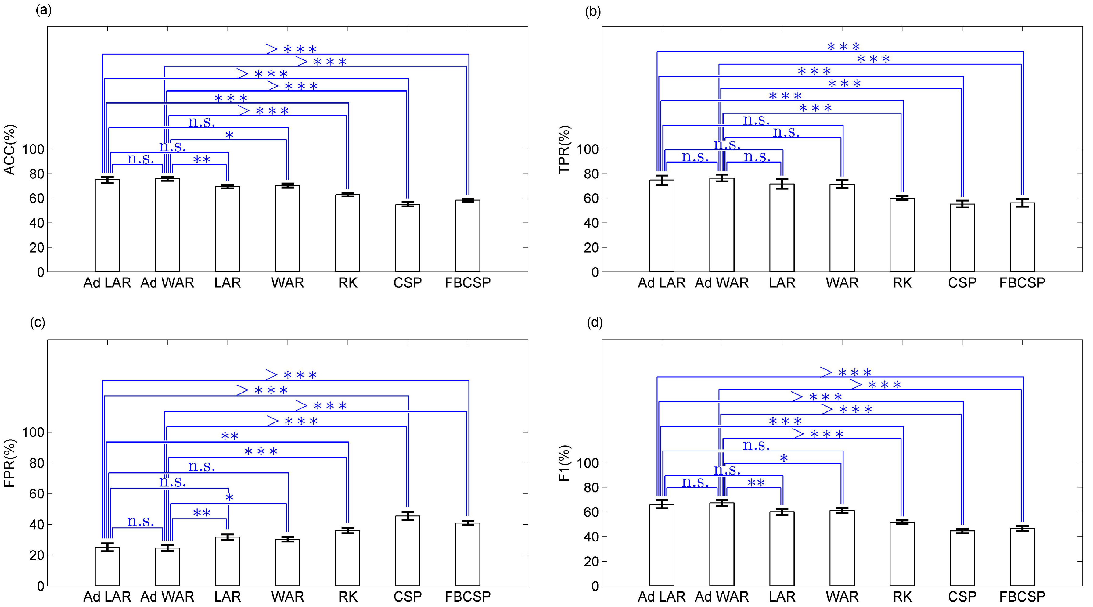
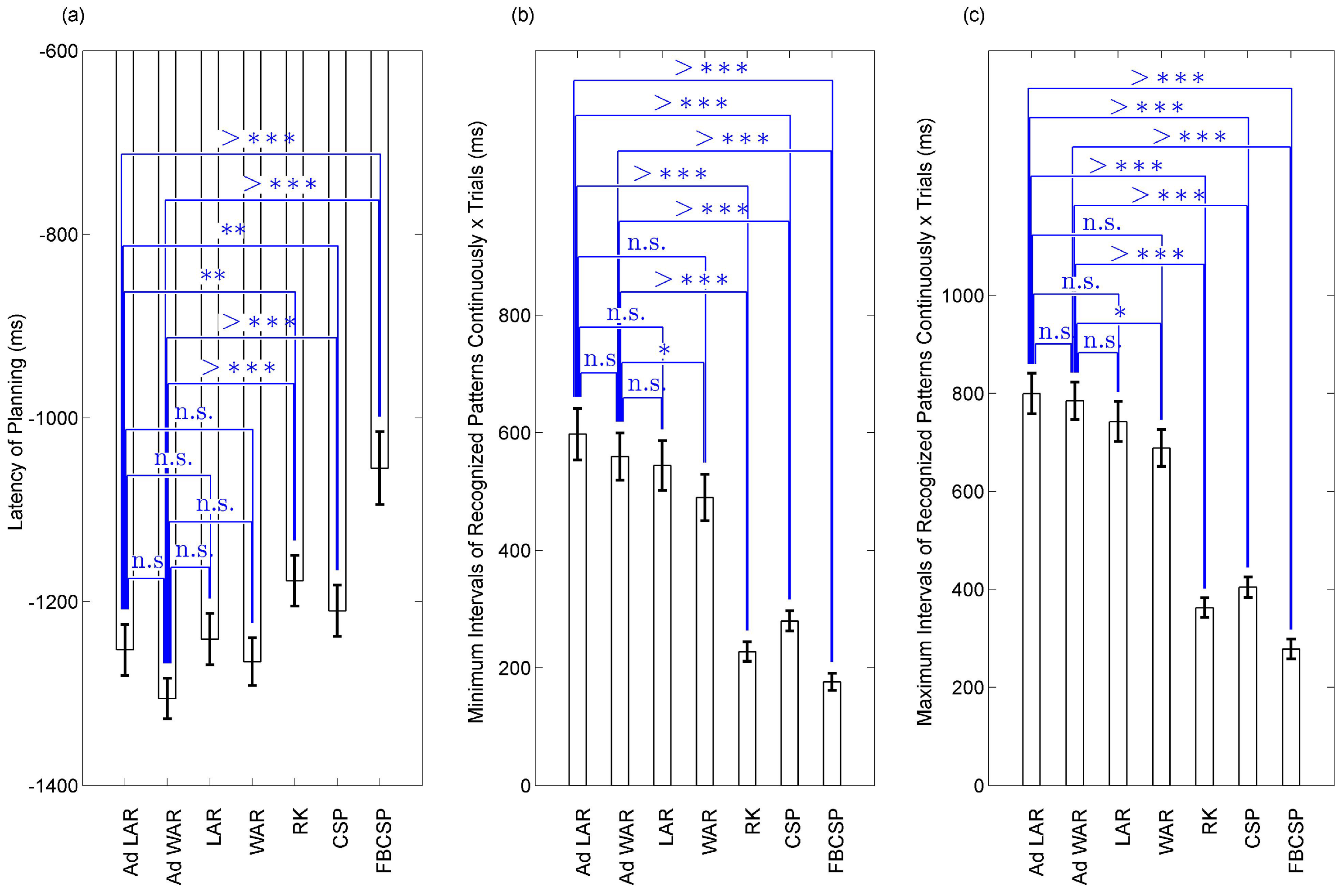
3.2. BCIs for Gait Planning Recognition
4. Discussion
Acknowledgments
Author Contributions
Conflicts of Interest
Appendix A. Feature Extraction from Riemannian Kernel
- Let and be the training and validation set, respectively.
- and are the bandpass filtered EEG from the training and validation set, respectively.
- Computing the Riemannian mean
- Spatial feature extraction
- Spatial feature extraction
Appendix B. Feature Extraction through Common Spatial Pattern
- Let and be the training and validation set, respectively.
- Defining a cross-validation 10-fold on the full training set , to obtain combinations of new training and testing set
- For = 1 to 10
- and are the bandpass filtered EEG.
- Getting patterns labeled as class 1 and 2 from
- = CSP(class1,class2); Computing the CSP projection matrix
- For m = 2 to 4
- holding the first and last m rows
- normalized common feature
- normalized common feature
- Applying the normal normalization of both , using the mean and standard deviation values of to normalize
- Applying Idx = LDA;
- Holding the that increases (see Equation (14)), improving the BCI performance
- Repeat until m = 4
- Repeat until = 10
- Filtering and
Appendix C. Feature Extraction using Filter-Bank Common Spatial Pattern
- Let and are the training and validation set, respectively.
- Defining a cross-validation 10-fold on the full training set , to obtain combinations of new training and testing set
- For = 1 to 10
- For b = 1 to 7
- and are the bandpass filtered EEG.
- Selecting classes 1 and 2 from
- = CSP(class1,class2); Computing the CSP projection matrix
- For m = 2 to 4
- holding the first and last m rows
- normalized common feature
- normalized common feature
- holding the features
- holding the features
- Repeat until m = 4
- Repeat until b = 7
- Evaluation of the feature set for each m
- For m = 2 to 4
- Applying the normal normalization of both , using the mean and standard deviation values of for
- Looking for the best first k features
- for k = 1 to
- Applying Idx = LDA;
- Holding the , and the best individual features that increase (see Equation (14)), improving the BCI performance
- Repeat until
- Repeat until m = 4
- Repeat until = 10
- For b = 1 to 7
- Filtering and
- normalized common feature
- normalized common feature
- holding
- holding
- Repeat until b = 7
- Selecting on and the best individual features obtained from the cross-validation
References
- Jiang, N.; Gizzi, L.; Mrachacz-Kersting, N.; Dremstrup, K.; Farina, D. A brain-computer interface for single-trial detection of gait initiation from movement related cortical potentials. Clin. Neurophysiol. 2015, 126, 154–159. [Google Scholar] [CrossRef] [PubMed]
- Xu, R.; Jiang, N.; Lin, C.; Mrachacz-Kersting, N.; Dremstrup, K.; Farina, D. Enhanced low-latency detection of motor intention from EEG for closed-loop brain-computer interface applications. IEEE Trans. Biomed. Eng. 2014, 61, 288–296. [Google Scholar] [PubMed]
- Hashimoto, Y.; Ushiba, J. EEG-based classification of imaginary left and right foot movements using beta rebound. Clin. Neurophysiol. 2013, 124, 2153–2160. [Google Scholar] [CrossRef] [PubMed]
- Gallego, J.Á.; Ibanez, J.; Dideriksen, J.L.; Serrano, J.I.; del Castillo, M.D.; Farina, D.; Rocon, E. A multimodal human–robot interface to drive a neuroprosthesis for tremor management. IEEE Trans. Syst. Man Cybern. Part C 2012, 42, 1159–1168. [Google Scholar] [CrossRef]
- Hortal, E.; Úbeda, A.; Iáñez, E.; Azorín, J.M.; Fernández, E. EEG-Based Detection of Starting and Stopping During Gait Cycle. Int. J. Neural Syst. 2016, 26, 1650029. [Google Scholar] [CrossRef] [PubMed]
- Wolpaw, J.R.; Birbaumer, N.; Heetderks, W.J.; McFarland, D.J.; Peckham, P.H.; Schalk, G.; Donchin, E.; Quatrano, L.A.; Robinson, C.J.; Vaughan, T.M. Brain-computer interface technology: A review of the first international meeting. IEEE Trans. Rehabil. Eng. 2000, 8, 164–173. [Google Scholar] [CrossRef] [PubMed]
- Pfurtscheller, G.; Flotzinger, D.; Kalcher, J. Brain-computer interface—A new communication device for handicapped persons. J. Microcomput. Appl. 1993, 16, 293–299. [Google Scholar] [CrossRef]
- Wolpaw, J.R.; McFarland, D.J. Multichannel EEG-based brain-computer communication. Electroencephalogr. Clin. Neurophysiol. 1994, 90, 444–449. [Google Scholar] [CrossRef]
- McFarland, D.J.; McCane, L.M.; David, S.V.; Wolpaw, J.R. Spatial filter selection for EEG-based communication. Electroencephalogr. Clin. Neurophysiol. 1997, 103, 386–394. [Google Scholar] [CrossRef]
- Wolpaw, J.R.; McFarland, D.J.; Neat, G.W.; Forneris, C.A. An EEG-based brain-computer interface for cursor control. Electroencephalogr. Clin. Neurophysiol. 1991, 78, 252–259. [Google Scholar] [CrossRef]
- Alshbatat, A.I.N.; Vial, P.J.; Premaratne, P.; Tran, L.C. EEG-based brain-computer interface for automating home appliances. J. Comput. 2014, 9, 2159–2166. [Google Scholar] [CrossRef]
- Müller, S.M.T.; Bastos, T.F.; Sarcinelli Filho, M. Proposal of a SSVEP-BCI to command a robotic wheelchair. J. Control Autom. Electr. Syst. 2013, 24, 97–105. [Google Scholar] [CrossRef]
- Diez, P.F.; Müller, S.M.T.; Mut, V.A.; Laciar, E.; Avila, E.; Bastos-Filho, T.F.; Sarcinelli-Filho, M. Commanding a robotic wheelchair with a high-frequency steady-state visual evoked potential based brain–Computer interface. Med. Eng. Phys. 2013, 35, 1155–1164. [Google Scholar] [CrossRef] [PubMed]
- Rocon, E.; Gallego, J.; Barrios, L.; Victoria, A.; Ibanez, J.; Farina, D.; Negro, F.; Dideriksen, J.L.; Conforto, S.; D’Alessio, T.; et al. Multimodal BCI-mediated FES suppression of pathological tremor. In Proceedings of the 2010 Annual International Conference Engineering in Medicine and Biology Society (EMBC), Buenos Aires, Argentina, 31 August–4 September 2010; pp. 3337–3340. [Google Scholar]
- Blankertz, B.; Tomioka, R.; Lemm, S.; Kawanabe, M.; Muller, K.R. Optimizing spatial filters for robust EEG single-trial analysis. IEEE Signal Proce. Mag. 2008, 25, 41–56. [Google Scholar] [CrossRef]
- Müller-Gerking, J.; Pfurtscheller, G.; Flyvbjerg, H. Designing optimal spatial filters for single-trial EEG classification in a movement task. Clin. Neurophysiol. 1999, 110, 787–798. [Google Scholar] [CrossRef]
- Ang, K.K.; Chin, Z.Y.; Wang, C.; Guan, C.; Zhang, H. Filter bank common spatial pattern algorithm on BCI competition IV datasets 2a and 2b. Front. Neurosci. 2012, 6, 39. [Google Scholar] [CrossRef] [PubMed]
- Barachant, A.; Bonnet, S.; Congedo, M.; Jutten, C. Classification of covariance matrices using a Riemannian-based kernel for BCI applications. Neurocomputing 2013, 112, 172–178. [Google Scholar] [CrossRef]
- Sburlea, A.I.; Montesano, L.; Minguez, J. Continuous detection of the self-initiated walking pre-movement state from EEG correlates without session-to-session recalibration. J. Neural Eng. 2015, 12, 036007. [Google Scholar] [CrossRef] [PubMed]
- Velu, P.D.; de Sa, V.R. Single-trial classification of gait and point movement preparation from human EEG. Front. Neurosci. 2013, 7, 84. [Google Scholar] [CrossRef] [PubMed]
- Kilicarslan, A.; Grossman, R.G.; Contreras-Vidal, J.L. A robust adaptive denoising framework for real-time artifact removal in scalp EEG measurements. J. Neural Eng. 2016, 13, 026013. [Google Scholar] [CrossRef] [PubMed]
- Schlögl, A.; Keinrath, C.; Zimmermann, D.; Scherer, R.; Leeb, R.; Pfurtscheller, G. A fully automated correction method of EOG artifacts in EEG recordings. Clin. Neurophysiol. 2007, 118, 98–104. [Google Scholar] [CrossRef] [PubMed]
- Daly, I.; Scherer, R.; Billinger, M.; Müller-Putz, G. FORCe: Fully Online and automated artifact Removal for brain-Computer interfacing. IEEE Trans. Neural Syst. Rehabil. Eng. 2015, 23, 725–736. [Google Scholar] [CrossRef] [PubMed]
- Urigüen, J.A.; Garcia-Zapirain, B. EEG artifact removal—State-of-the-art and guidelines. J. Neural Eng. 2015, 12, 031001. [Google Scholar] [CrossRef] [PubMed]
- Puthusserypady, S.; Ratnarajah, T. H/sup/spl infin//adaptive filters for eye blink artifact minimization from electroencephalogram. IEEE Signal Process. Lett. 2005, 12, 816–819. [Google Scholar] [CrossRef]
- Guerrero-Mosquera, C.; Navia-Vázquez, A. Automatic removal of ocular artefacts using adaptive filtering and independent component analysis for electroencephalogram data. IET Signal Process. 2012, 6, 99–106. [Google Scholar] [CrossRef]
- Khatun, S.; Mahajan, R.; Morshed, B.I. Comparative study of wavelet-based unsupervised ocular artifact removal techniques for single-channel EEG data. IEEE J. Transl. Eng. Health Med. 2016, 4, 1–8. [Google Scholar] [CrossRef] [PubMed]
- Pfurtscheller, G.; Da Silva, F.L. Event-related EEG/MEG synchronization and desynchronization: Basic principles. Clin. Neurophysiol. 1999, 110, 1842–1857. [Google Scholar] [CrossRef]
- Pfurtscheller, G.; Neuper, C.; Berger, J. Source localization using eventrelated desynchronization (ERD) within the alpha band. Brain Topogr. 1994, 6, 269–275. [Google Scholar] [CrossRef] [PubMed]
- Jung, T.P.; Humphries, C.; Lee, T.W.; Makeig, S.; McKeown, M.J.; Iragui, V.; Sejnowski, T.J. Extended ICA removes artifacts from electroencephalographic recordings. In Proceedings of the Advances in Neural Information Processing Systems, Denver, CO, USA, 30 November–5 December 1998; pp. 894–900. [Google Scholar]
- Jung, T.P.; Humphries, C.; Lee, T.W.; Makeig, S.; McKeown, M.J.; Iragui, V.; Sejnowski, T.J. Removing electroencephalographic artifacts: Comparison between ICA and PCA. In Proceedings of the 1998 IEEE Signal Processing Society Workshop Neural Networks for Signal Processing VIII, Cambridge, UK, 2 September 1998; pp. 63–72. [Google Scholar]
- Seeber, M.; Scherer, R.; Wagner, J.; Solis-Escalante, T.; Müller-Putz, G.R. High and low gamma EEG oscillations in central sensorimotor areas are conversely modulated during the human gait cycle. Neuroimage 2015, 112, 318–326. [Google Scholar] [CrossRef] [PubMed]
- Mullen, T.; Kothe, C.; Chi, Y.M.; Ojeda, A.; Kerth, T.; Makeig, S.; Cauwenberghs, G.; Jung, T.P. Real-time modeling and 3D visualization of source dynamics and connectivity using wearable EEG. In Proceedings of the 2013 35th Annual International Conference of the IEEE Engineering in Medicine and Biology Society (EMBC), Osaka, Japan, 3–7 July 2013; pp. 2184–2187. [Google Scholar]
- Vaseghi, S.V. Advanced Digital Signal Processing and Noise Reduction; John Wiley & Sons: Hoboken, NJ, USA, 2008. [Google Scholar]
- Sweeney, K.T.; Ayaz, H.; Ward, T.E.; Izzetoglu, M.; McLoone, S.F.; Onaral, B. A methodology for validating artifact removal techniques for physiological signals. IEEE Trans. Inf. Technol. Biomed. 2012, 16, 918–926. [Google Scholar] [CrossRef] [PubMed]
- Sweeney, K.T.; McLoone, S.F.; Ward, T.E. The use of ensemble empirical mode decomposition with canonical correlation analysis as a novel artifact removal technique. IEEE Trans. Biomed. Eng. 2013, 60, 97–105. [Google Scholar] [CrossRef] [PubMed]
- Lawrence, I.; Lin, K. A concordance correlation coefficient to evaluate reproducibility. Biometrics 1989, 45, 255–268. [Google Scholar]
- Villa-Parra, A.; Delisle-Rodríguez, D.; López-Delis, A.; Bastos-Filho, T.; Sagaró, R.; Frizera-Neto, A. Towards a robotic knee exoskeleton control based on human motion intention through EEG and sEMGsignals. Proced. Manuf. 2015, 3, 1379–1386. [Google Scholar] [CrossRef]
- Laplante, P.A. Electrical Engineering Dictionary; CRC Press LLC.: Boca Raton, FL, USA, 2000. [Google Scholar]
- Chen, X.; Wang, Y.; Gao, S.; Jung, T.P.; Gao, X. Filter bank canonical correlation analysis for implementing a high-speed SSVEP-based brain–computer interface. J. Neural Eng. 2015, 12, 046008. [Google Scholar] [CrossRef] [PubMed]
- Cotrina, A.; Benevides, A.B.; Castillo-Garcia, J.; Benevides, A.B.; Rojas-Vigo, D.; Ferreira, A.; Bastos-Filho, T.F. A SSVEP-BCI Setup Based on Depth-of-Field. IEEE Trans. Neural Syst. Rehabil. Eng. 2017, 25, 1047–1057. [Google Scholar] [CrossRef] [PubMed]
- Quiroga, R.Q.; Kraskov, A.; Kreuz, T.; Grassberger, P. Performance of different synchronization measures in real data: A case study on electroencephalographic signals. Phys. Rev. E 2002, 65, 041903. [Google Scholar] [CrossRef] [PubMed]
- Lin, Z.; Zhang, C.; Wu, W.; Gao, X. Frequency recognition based on canonical correlation analysis for SSVEP-based BCIs. IEEE Trans. Biomed. Eng. 2007, 54, 1172–1176. [Google Scholar] [CrossRef] [PubMed]
- Japkowicz, N.; Shah, M. Evaluating Learning Algorithms: A Classification Perspective; Cambridge University Press: Cambridge, UK, 2011. [Google Scholar]
- McFarland, D.J.; Anderson, C.W.; Muller, K.R.; Schlogl, A.; Krusienski, D.J. BCI meeting 2005-workshop on BCI signal processing: Feature extraction and translation. IEEE Trans. Neural Syst. Rehabil. Eng. 2006, 14, 135–138. [Google Scholar] [CrossRef] [PubMed]
- Qin, L.; Ding, L.; He, B. Motor imagery classification by means of source analysis for brain–computer interface applications. J. Neural Eng. 2004, 1, 135. [Google Scholar] [CrossRef] [PubMed]
- Lemm, S.; Blankertz, B.; Curio, G.; Muller, K.R. Spatio-spectral filters for improving the classification of single trial EEG. IEEE Trans. Biomed. Eng. 2005, 52, 1541–1548. [Google Scholar] [CrossRef] [PubMed]
- Phothisonothai, M.; Watanabe, K. Optimal fractal feature and neural network: EEG based BCI applications. In Brain-Computer Interface Systems-Recent Progress and Future Prospects; InTech: Rijeka, Croatia, 2013. [Google Scholar]
- Liu, J.; Yang, Q.; Yao, B.; Brown, R.; Yue, G. Linear correlation between fractal dimension of EEG signal and handgrip force. Biol. Cybern. 2005, 93, 131–140. [Google Scholar] [CrossRef] [PubMed]
- Delisle-Rodriguez, D.; Villa-Parra, A.C.; López-Delis, A.; Frizera-Neto, A.; Rocon, E.; Freire-Bastos, T. Non-supervised Feature Selection: Evaluation in a BCI for Single-Trial Recognition of Gait Preparation/Stop. In Converging Clinical and Engineering Research on Neurorehabilitation II; Springer: Berlin, Germany, 2017; pp. 1115–1120. [Google Scholar]
- Mitra, P.; Murthy, C.; Pal, S.K. Unsupervised feature selection using feature similarity. IEEE Trans. Pattern Anal. Mach. Intell. 2002, 24, 301–312. [Google Scholar] [CrossRef]
- Castro, M.C.F.; Arjunan, S.P.; Kumar, D.K. Selection of suitable hand gestures for reliable myoelectric human computer interface. Biomed. Eng. Online 2015, 14, 30. [Google Scholar] [CrossRef] [PubMed]
- Lew, E.; Chavarriaga, R.; Silvoni, S.; Millán, J.d.R. Detection of self-paced reaching movement intention from EEG signals. Front. Neuroeng. 2012, 5, 13. [Google Scholar] [CrossRef] [PubMed]
- Schlögl, A.; Brunner, C. BioSig: A free and open source software library for BCI research. Computer 2008, 41, 44–50. [Google Scholar] [CrossRef]
- Jain, A.K.; Duin, R.P.W.; Mao, J. Statistical pattern recognition: A review. IEEE Trans. Pattern Anal. Mach. Intell. 2000, 22, 4–37. [Google Scholar] [CrossRef]


| Subj | SVM (CFS) | ACC(%) | TPR(%) | FPR(%) | F1(%) | Latency (ms) |
|---|---|---|---|---|---|---|
| S1 | 0.053 | |||||
| S2 | 0.011*, 0.52 | |||||
| S3 | 0.013 | |||||
| S4 | 0.013 | |||||
| S5 | 0.13 | |||||
| S6 | 0.013 |
| Subj | SVM (CFS) | ACC(%) | TPR(%) | FPR(%) | F1(%) | Latency (ms) |
|---|---|---|---|---|---|---|
| S1 | 0.13 | |||||
| S2 | 0.012*,0.05 | |||||
| S3 | 0.13 | |||||
| S4 | 0.01,0.05,0.5 | |||||
| S5 | 0.013 | |||||
| S6 | 0.01,0.52* |
| Sub | Ad LAR | RE | Ad WAR | RE | CSP | FBCSP | RK | |||
|---|---|---|---|---|---|---|---|---|---|---|
| Original Features (Size) | Selected Features (Size) | Original Features (Size) | Selected Features (Size) | m | Features (Size) | m | k | Selected Features (Size) | Features (Size) | |
| S1 | 36 | 23–34 | 36 | 24–29 | 4 | 8 | 3–4 | 12 | 24–32 | 36 |
| S2 | 36 | 20–25 | 36 | 24–26 | 4 | 8 | 3–4 | 12 | 16–24 | 36 |
| S3 | 36 | 21–22 | 36 | 27–28 | 3–4 | 6–8 | 4 | 12 | 16–32 | 36 |
| S4 | 36 | 24–25 | 36 | 20–28 | 4 | 8 | 4 | 12 | 16–24 | 36 |
| S5 | 36 | 26–30 | 36 | 21–32 | 3–4 | 6–8 | 4 | 12 | 16–24 | 36 |
| S6 | 36 | 27–32 | 36 | 20–24 | 3–4 | 6–8 | 3–4 | 12 | 16–34 | 36 |
© 2017 by the authors. Licensee MDPI, Basel, Switzerland. This article is an open access article distributed under the terms and conditions of the Creative Commons Attribution (CC BY) license (http://creativecommons.org/licenses/by/4.0/).
Share and Cite
Delisle-Rodriguez, D.; Villa-Parra, A.C.; Bastos-Filho, T.; López-Delis, A.; Frizera-Neto, A.; Krishnan, S.; Rocon, E. Adaptive Spatial Filter Based on Similarity Indices to Preserve the Neural Information on EEG Signals during On-Line Processing. Sensors 2017, 17, 2725. https://doi.org/10.3390/s17122725
Delisle-Rodriguez D, Villa-Parra AC, Bastos-Filho T, López-Delis A, Frizera-Neto A, Krishnan S, Rocon E. Adaptive Spatial Filter Based on Similarity Indices to Preserve the Neural Information on EEG Signals during On-Line Processing. Sensors. 2017; 17(12):2725. https://doi.org/10.3390/s17122725
Chicago/Turabian StyleDelisle-Rodriguez, Denis, Ana Cecilia Villa-Parra, Teodiano Bastos-Filho, Alberto López-Delis, Anselmo Frizera-Neto, Sridhar Krishnan, and Eduardo Rocon. 2017. "Adaptive Spatial Filter Based on Similarity Indices to Preserve the Neural Information on EEG Signals during On-Line Processing" Sensors 17, no. 12: 2725. https://doi.org/10.3390/s17122725