Terahertz Spectroscopy for Proximal Soil Sensing: An Approach to Particle Size Analysis


Abstract
:1. Introduction
- -
- How does the particle size influence the spectral behavior, and is there a limit or saturation of the signal amplitudes?
- -
- How does the sand fraction, with a large particle size, interfere with the THz radiation (≈wavelength (λ))?
- -
- How does the sample thickness influence the spectral behavior?
- -
- Which fraction dominates the signal content of mixed fractions?
- -
- For the soil fractions, silt and clay, which are relevant for the adsorption of plant nutrients, high penetration by THz radiation is expected, because of the low Rayleigh scattering by fractions with particle sizes much smaller than the wavelength (<<λ). Thus the question is, do soils with similar textures differ in THz transmission?
2. Materials and Methods
2.1. Soil Samples
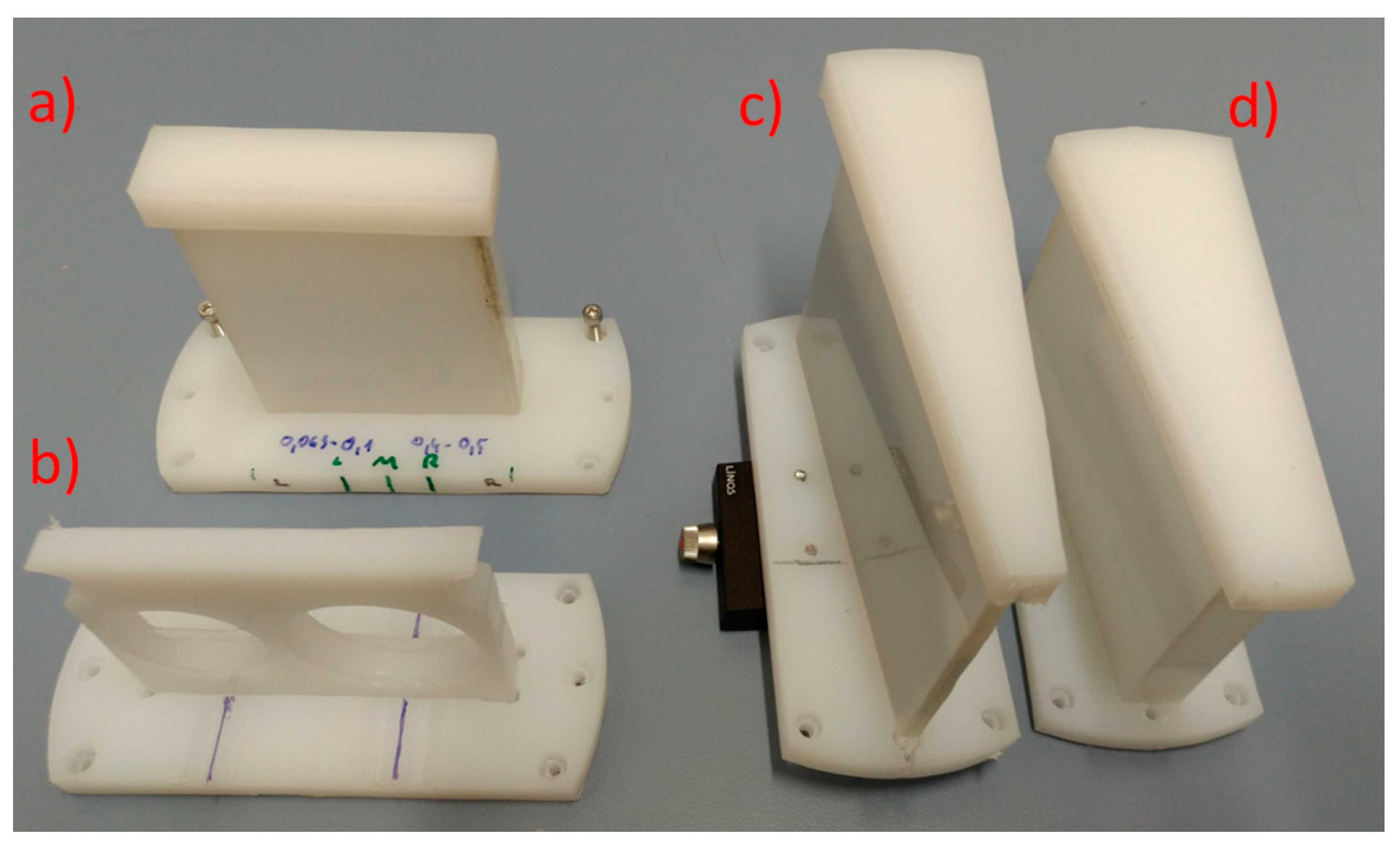
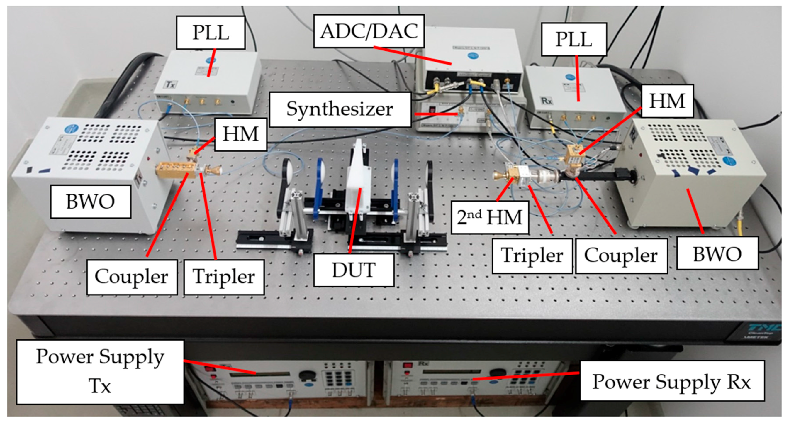
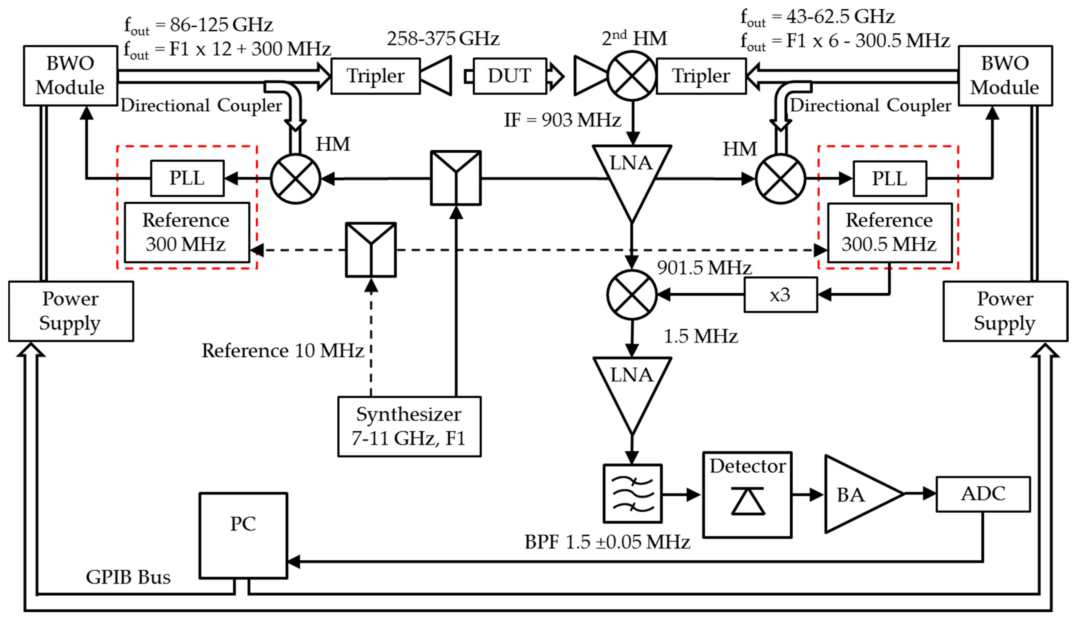
2.2. THz Setup
- -
- Setup 1: Rx-tube 1 with a second HM WR3.4SHM and ADC-preamp 1.
- -
- Setup 2: Rx-tube 2 with a second HM WR2.8SHM and ADC-preamp 2.
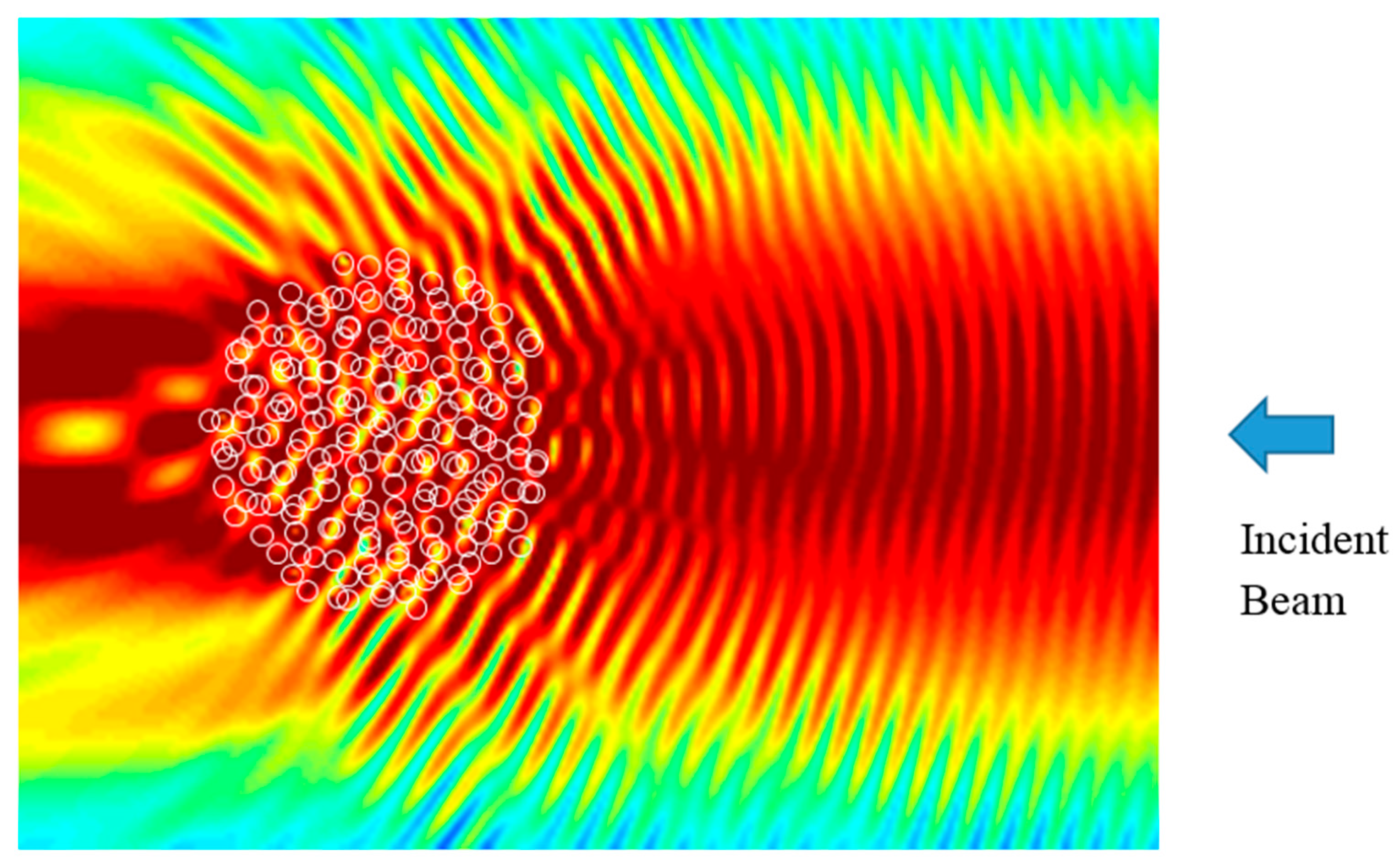
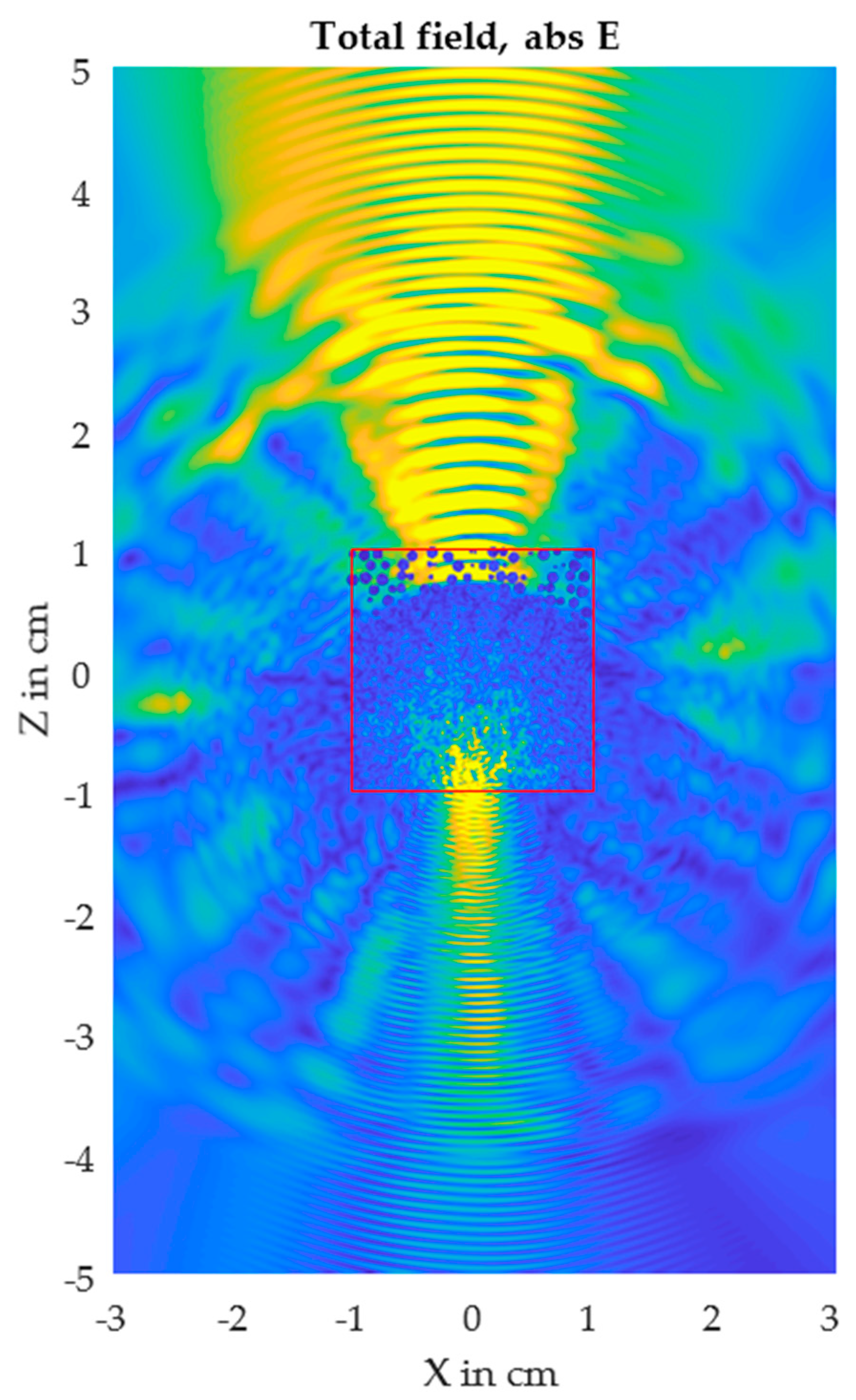
2.3. Scattering and Diffraction
2.3.1. Abbe’s Resolution Limit
2.3.2. Rayleigh Scattering
2.3.3. Mie Scattering
3. Results
3.1. Particle Size Dependency
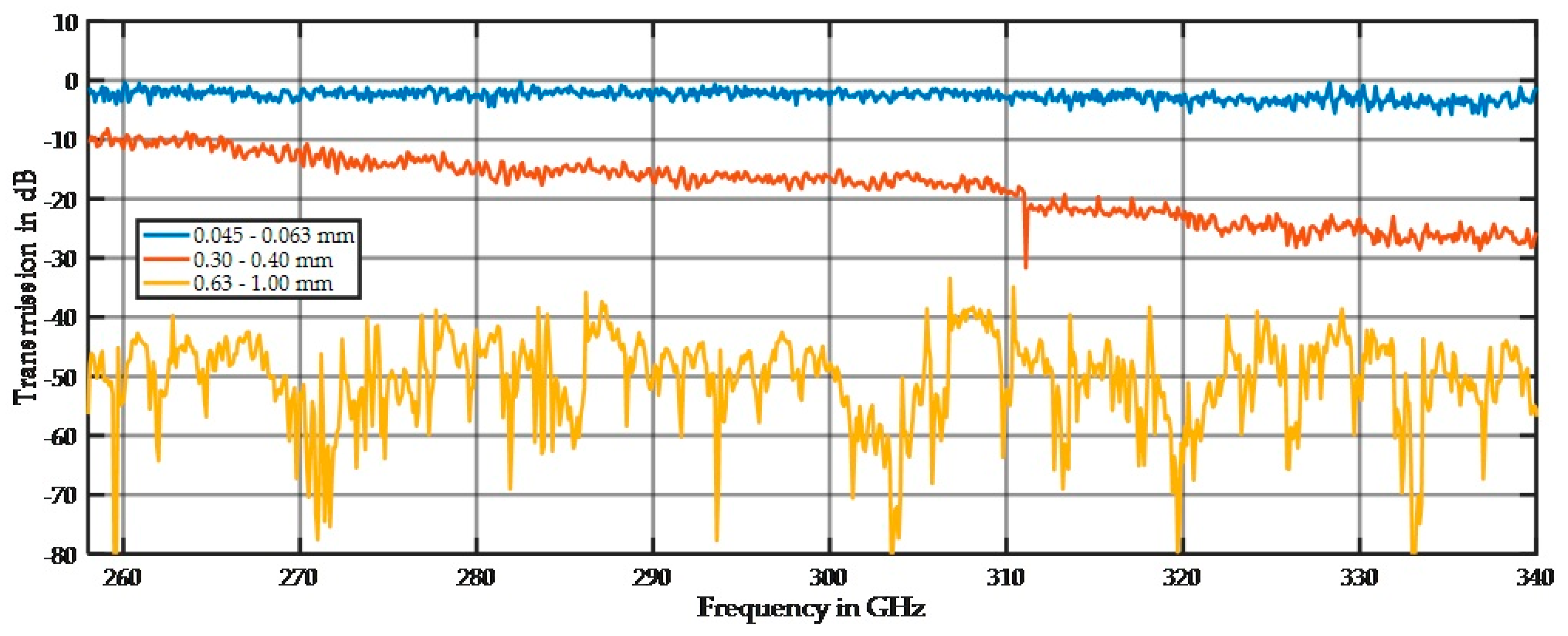
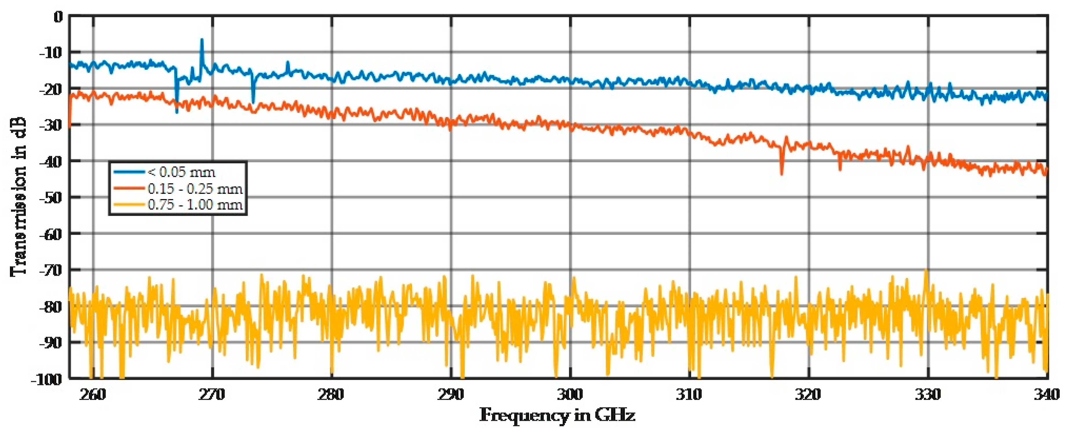
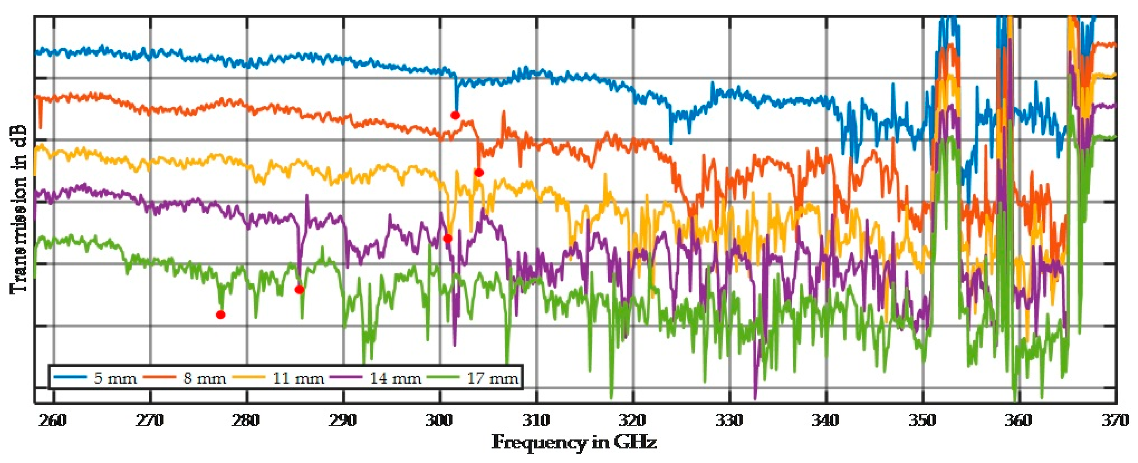
3.1.1. Spectral Behavior
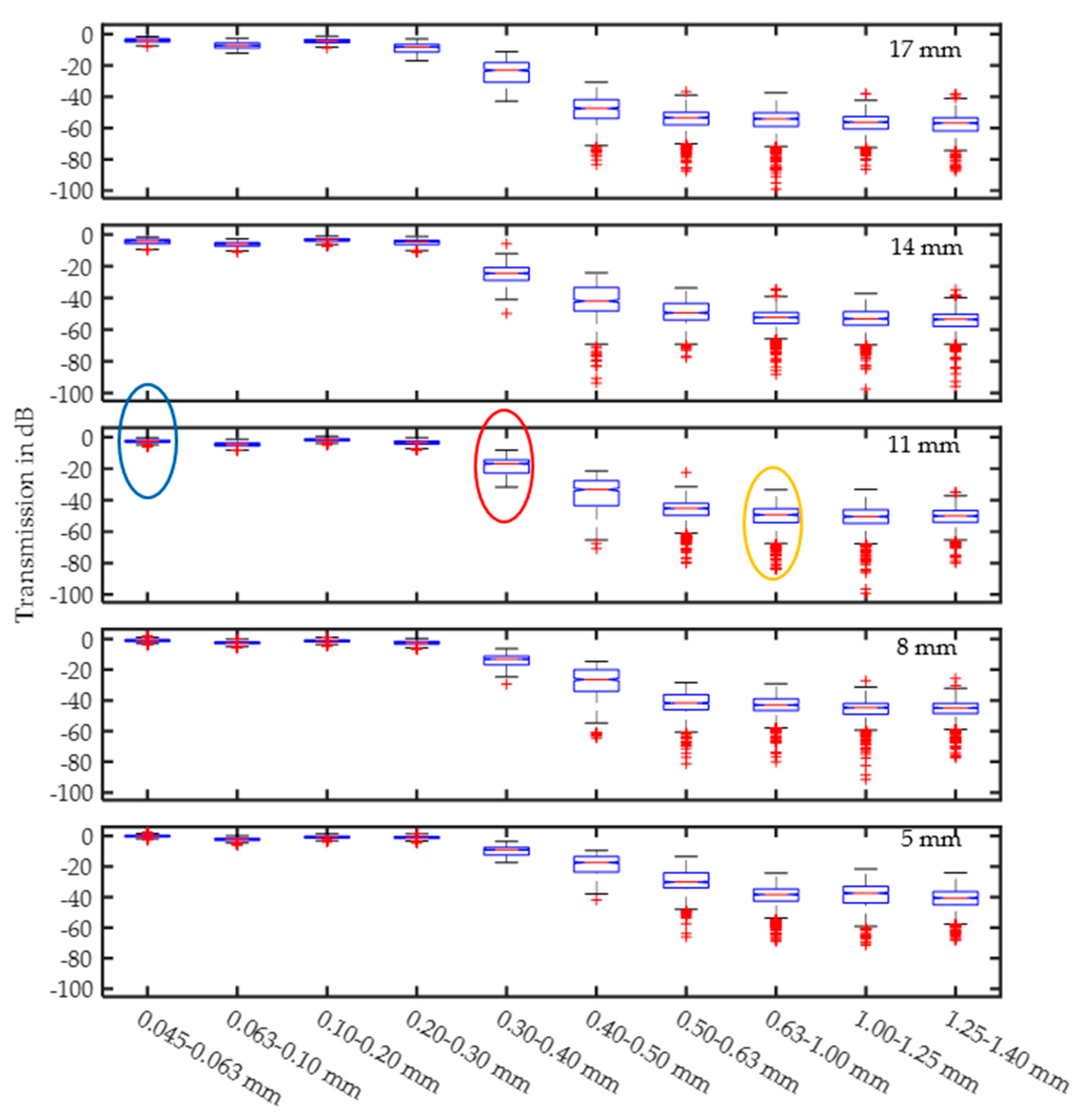
3.1.2. Damping Behavior
3.1.3. Particular Effects at the Half-Wavelength
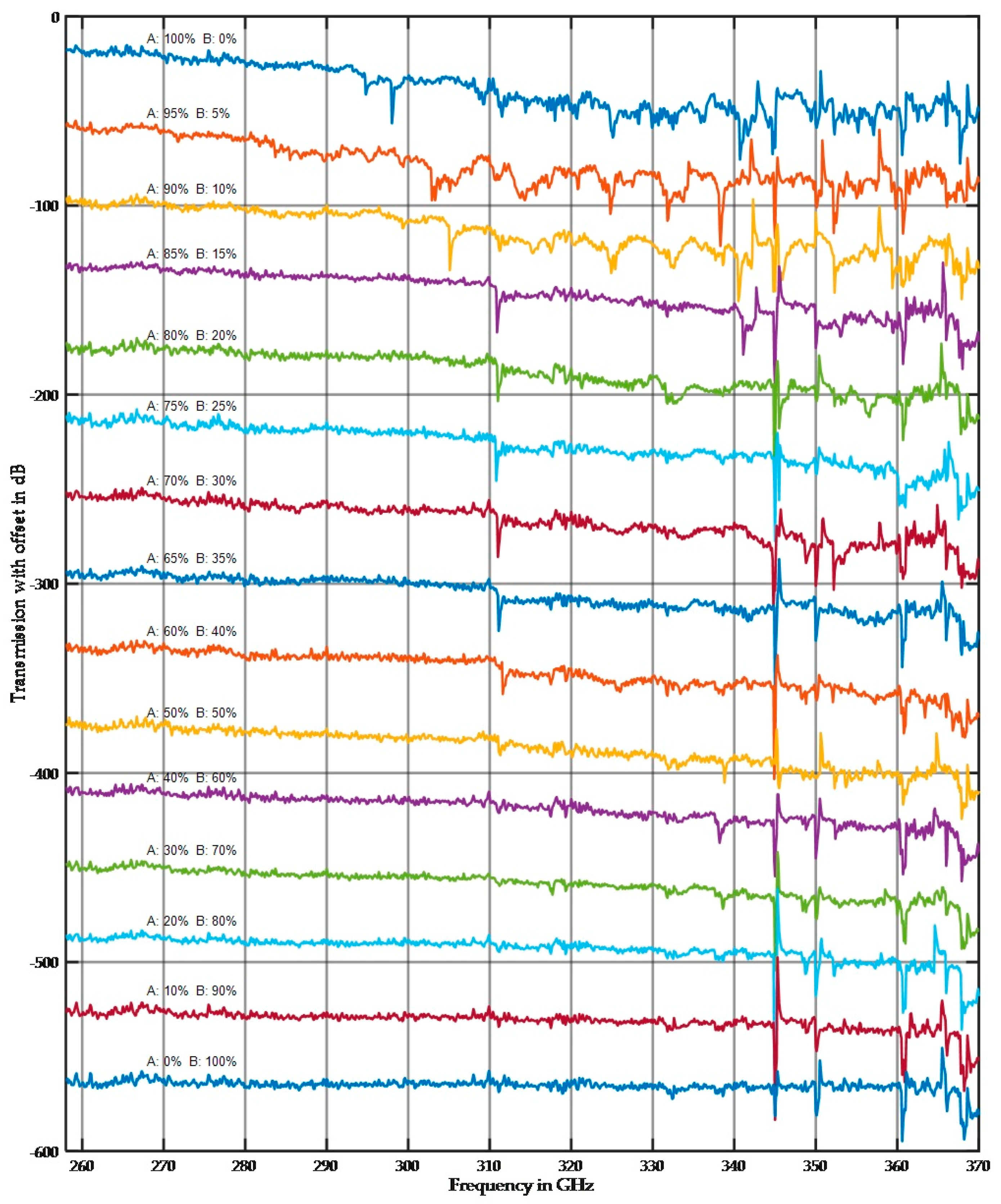
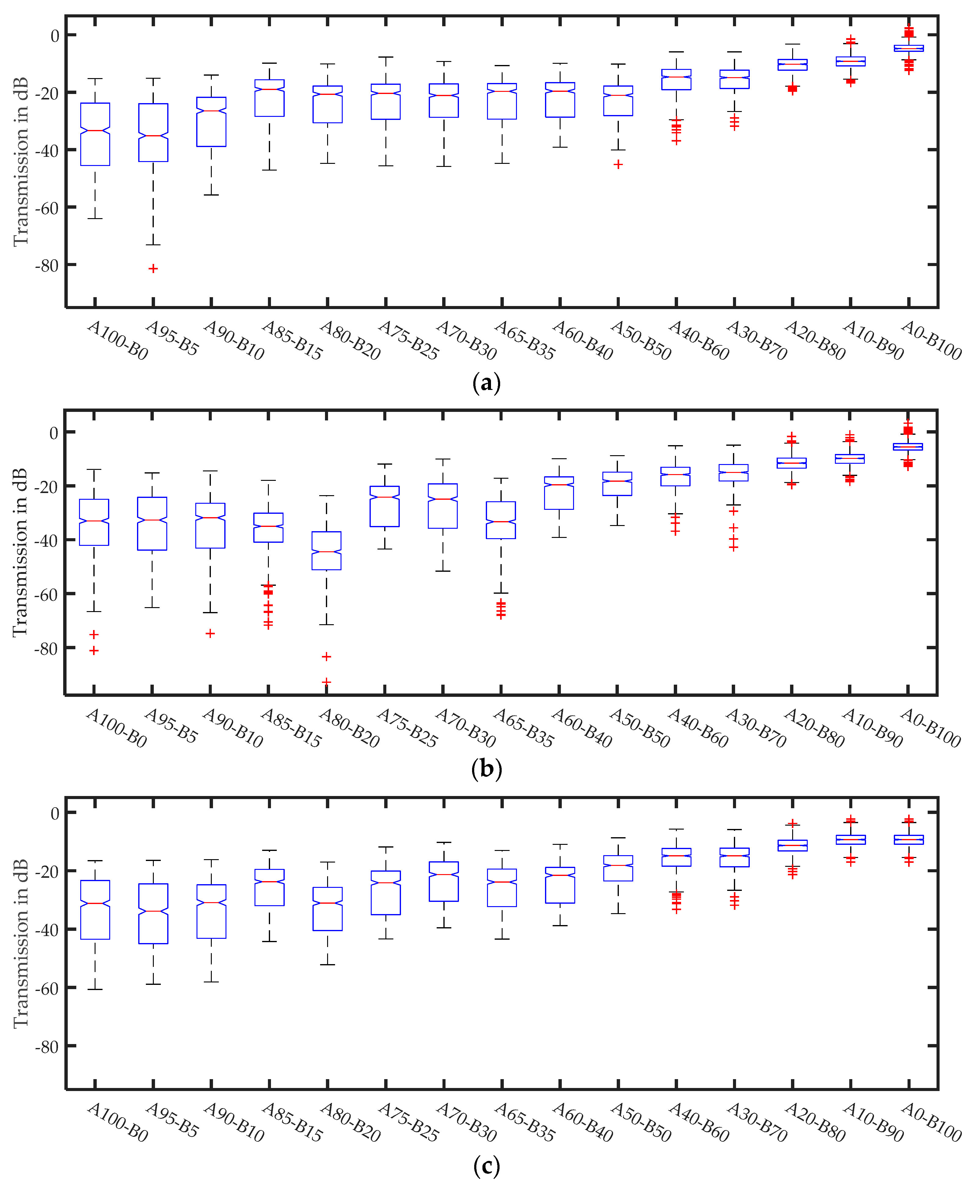
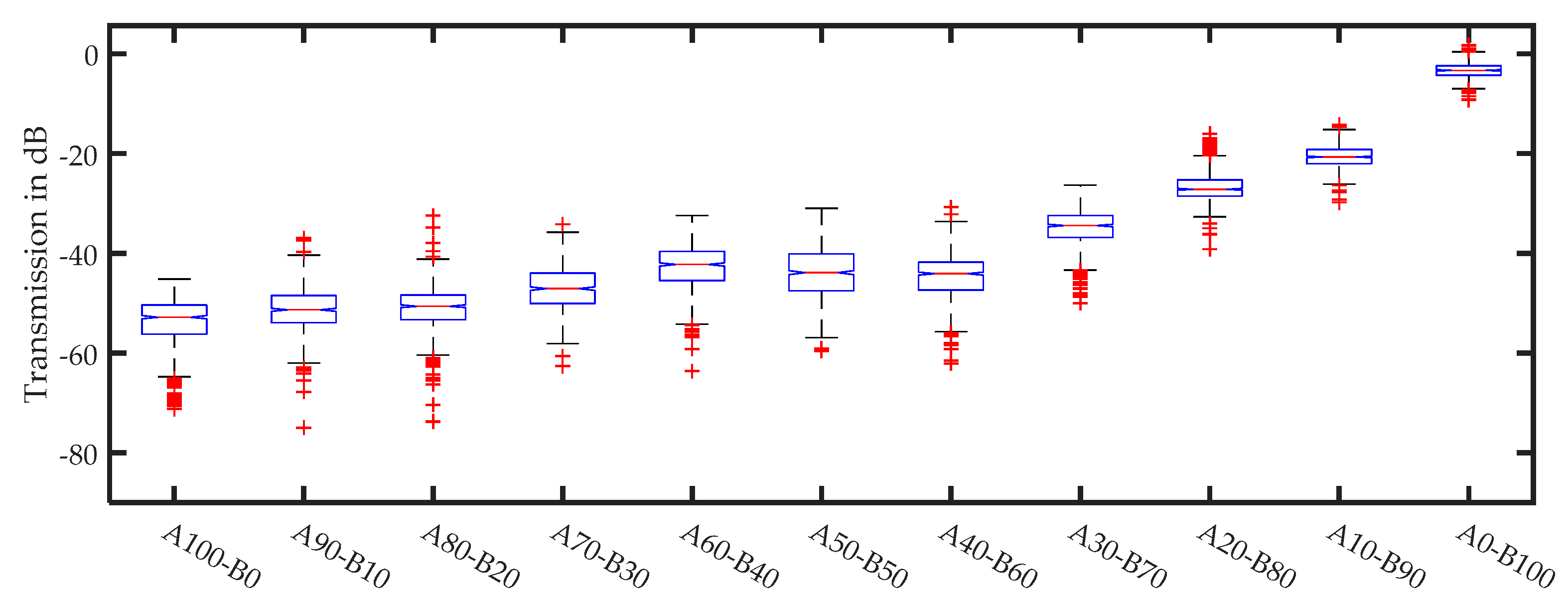
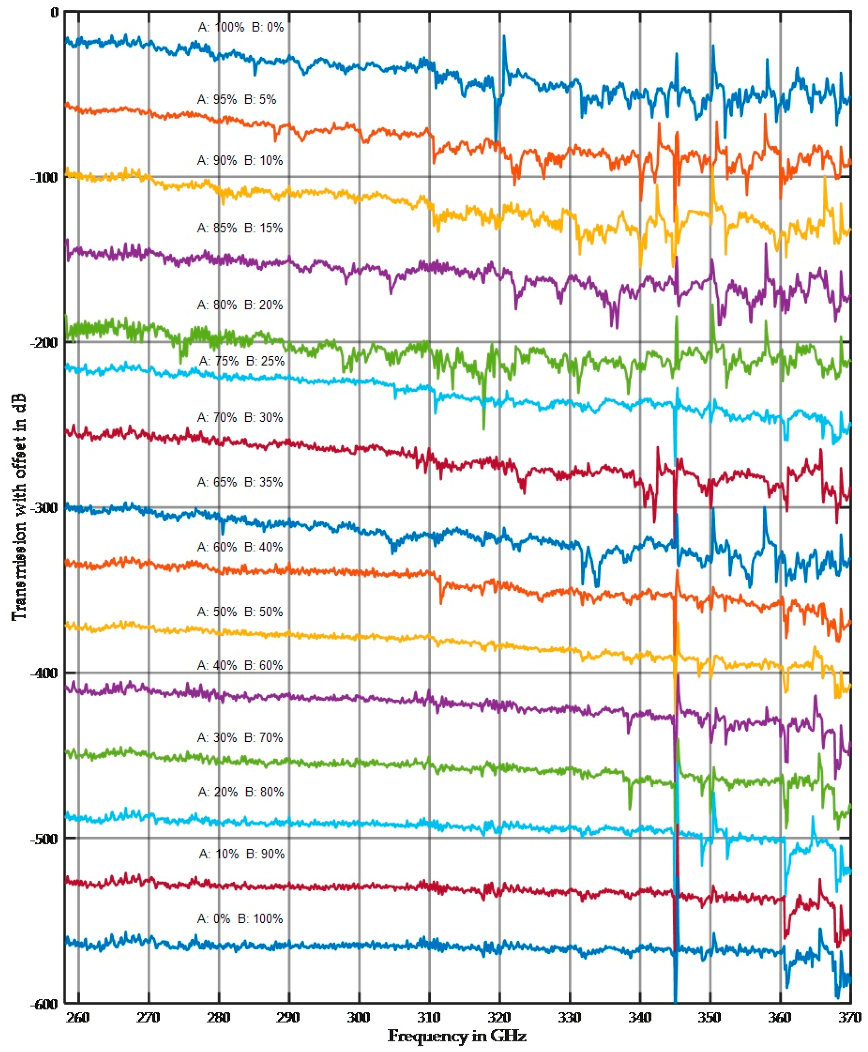
3.2. Mixed Fractions
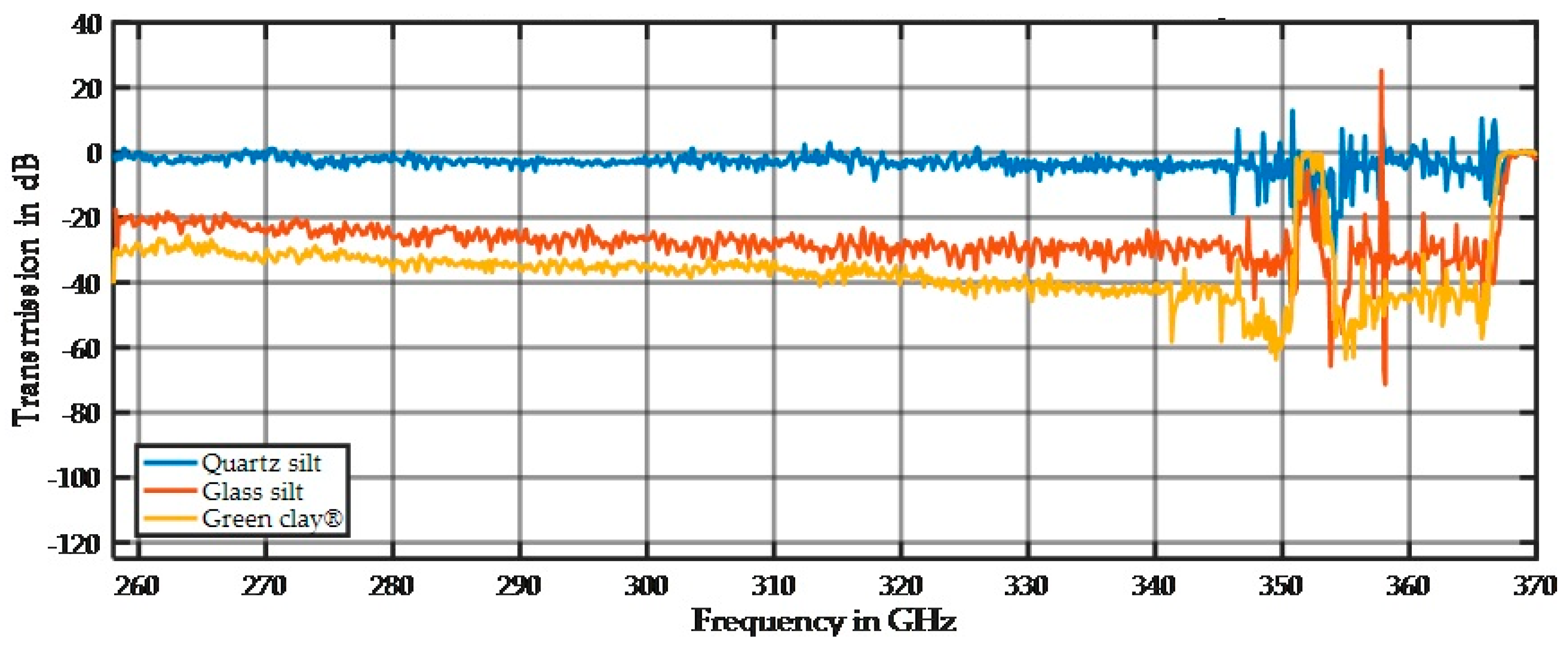
3.3. Material Content
4. Discussion
5. Conclusions
Acknowledgments
Author Contributions
Conflicts of Interest
Abbreviations
| Vis-NIR | visible to near-infrared |
| 2D | two-dimensional |
| HDPE | high-density polyethylene |
| THz | Terahertz |
| GHz | Gigahertz |
| pH | Potential hydrogen |
| XRF | Roentgen radiation fluorescence or X-ray fluorescence |
| BWO | Backward wave oscillator (tube) |
| CW | Continuous wave |
| HM | Harmonic mixer |
References
- Pätzold, S.; Mertens, F.M.; Bornemann, L.; Koleczek, B.; Franke, J.; Feilhauer, H.; Welp, G. Soil Heterogeneity at the Field Scale: A Challenge for Precision Crop Protection. Precis. Agric. 2008, 9, 367–390. [Google Scholar] [CrossRef]
- Dammer, K. Real-time variable-rate herbicide application for weed control in carrots. Weed Res. 2016, 56, 237–246. [Google Scholar] [CrossRef]
- Gebbers, R.; Tavakoli, H.; Herbst, R. Crop sensor readings in winter wheat as affected by nitrogen and water supply. In Precision Agriculture’13. 9th European Conference on Precision Agriculture; Stafford, J.V., Ed.; Wageningen Academic Publishers: Wageningen, The Netherlands, 2013; pp. 79–86. ISBN 978-90-8686-224-5. [Google Scholar]
- Selige, T.; Böhner, J.; Schmidhalter, U. High resolution topsoil mapping using hyper spectral image and field data in multivariate regression modelling procedures. Geoderma 2006, 136, 235–244. [Google Scholar] [CrossRef]
- Bochtis, D.D.; Sørensen, C.G.; Rasmus, N.J.; Nørremark, M.; Ibrahim, A.H.; Kishore, C.S. Robotic weed monitoring. Acta Agric. Scand. 2011, 61, 202–208. [Google Scholar] [CrossRef]
- Wallor, E.; Kersebaum, K.C.; Lorenz, K.; Gebbers, R. Connecting Crop Models with Highly Resolved Sensor Observations to Improve Site-Specific Fertilization. In Proceedings of the 11th European Conference on Precisin Agriculture (ECPA 2017), Edinburgh, UK, 16–20 July 2017; Volume 8, pp. 689–693. [Google Scholar]
- Gebbers, R.; Lück, E.; Rühlmann, J. (Eds.) (2013): 3rd Global Workshop on Proximal Soil Sensing 2013. International Union of Soil Sciences, Working Group on Proximal Soil Sensing. Bornimer Agrartechnische Berichte Heft 82; Leibnitz-Institut für Agrartechnik Potsdam-Bornim e.V.: Potsdam, Germany, 2013; ISSN 0947-7314. [Google Scholar]
- Viscarra Rossel, R.A.; Adamchuk, V.I.; Sudduth, K.A.; McKenzie, N.J.; Lobsey, C. Proximal Soil Sensing: An Effective Approach for Soil Measurements in Space and Time. Adv. Agron. 2011, 113, 237–282. [Google Scholar]
- Gebbers, R.; Schirrmann, M.; Kramer, E.; Seidel, J. Predicting lime requirements by fusion of proximal soil sensors. In Proceedings of the 8th conference on Precision Agriculture, Czech Centre of Science and Society, Prague, Czech Republic, 11–14 July 2011; pp. 562–576. [Google Scholar]
- Schirrmann, M.; Gebbers, R.; Kramer, E.; Seidel, J. Soil pH mapping with an on-the-go sensor. Sensors 2011, 1, 573–598. [Google Scholar] [CrossRef] [PubMed]
- Adamchuk, V.I.; Lund, E.D.; Sethuramasamyraja, B.; Morgan, M.T.; Dobermann, A.; Marx, D.B. Direct measurement of soil chemical properties on-the-go using ion-selective electrodes. Comput. Electron. Agric. 2005, 48, 272–294. [Google Scholar] [CrossRef]
- Domsch, H.; Boess, J.; Ehlert, D.; Wuttig, H. Evaluation of the penetration resistance along a transect. In Precision Agriculture’ 05. 5th European Conference on Precision Agriculture; Stafford, J., Ed.; Wageningen Acadamic Publishers: Wageningen, The Netherlands, 2005; pp. 465–472. [Google Scholar] [CrossRef]
- Lück, E.; Gebbers, R.; Rühlmann, J.; Spangenberg, U. Electrical conductivity mapping for precision farming. Near Surf. Geophys. 2009, 7, 15–25. [Google Scholar] [CrossRef]
- Lück, E.; Rühlmann, J. Resistivity mapping with GEOPHILUS ELECTRICUS—Information about lateral and vertical soil heterogeneity. Geoderma 2013, 199, 2–11. [Google Scholar] [CrossRef]
- Cook, P.G.; Walker, G.R. Depth Profiles of Electrical-Conductivity from Linear-Combinations of Electromagnetic Induction Measurements. Soil Sci. Soc. Am. J. 1992, 56, 1015–1022. [Google Scholar] [CrossRef]
- Singh, G.; Williard, K.W.J.; Schoonover, J.E. Spatial Relation of Apparent Soil Electrical Conductivity with Crop Yields and Soil Properties at Different Topographic Positions in a Small Agricultural Watershed. Agronomy 2016, 6, 57. [Google Scholar] [CrossRef]
- Rodionov, A.; Pätzold, S.; Welp, G.; Cañada Pallares, R.; Damerow, L.; Amelung, W. Sensing of soil organic carbon using VIS-NIR spectroscopy at variable moisture and surface roughness. Soil Sci. Soc. Am. J. 2014, 78, 949–957. [Google Scholar] [CrossRef]
- Imade Anom, S.W.; Shibusawa, S.; Sasao, A.; Hirako, S. Soil parameters maps in paddy field using the real time soil spectrophotometer. JSAM J. 2001, 63, 51–58. [Google Scholar]
- Kodaira, M.; Shibusawa, S. Using a mobile real-time soil visible-near infrared sensor for high resolution soil property mapping. Geoderma 2013, 199, 64–79. [Google Scholar] [CrossRef]
- O'Rourke, S.M.; Stockmann, U.; Holden, N.M.; McBratney, A.B.; Minasny, B. An assessment of model averaging to improve predictive power of portable VIS-NIR and XRF for the determination of agronomic soil properties. Geoderma 2016, 279, 31–44. [Google Scholar] [CrossRef]
- Dworak, V.; Augustin, S.; Gebbers, R. Application of Terahertz Radiation to Soil Measurements: Initial Results. Sensors 2011, 11, 9973–9988. [Google Scholar] [CrossRef] [PubMed]
- Lewis, R.A. Invited Review Terahertz Transmission, Scattering, Reflection and Absorption—The Interaction of THz Radiation with Soils. J. Infrared Millim. Terahertz Waves 2017, 38, 799–807. [Google Scholar] [CrossRef]
- Li, M.; Dai, G.; Chang, T.; Shi, C.; Wei, D.; Du, C.; Cui, H.-L. Accurate Determination of Geographical Origin of Tea Based on Terahertz Spectroscopy. Appl. Sci. 2017, 7, 172. [Google Scholar] [CrossRef]
- Takeya, K.; Muto, K.; Ishihara, Y.; Kawase, K. Monitoring Theophylline Concentrations in Saline Using Terahertz ATR Spectroscopy. Appl. Sci. 2016, 6, 72. [Google Scholar] [CrossRef]
- Kuroo, K.; Hasegawa, R.; Tanabe, T.; Oyama, Y. Terahertz Application for Non-Destructive Inspection of Coated Al Electrical Conductive Wires. J. Imaging 2017, 3, 27. [Google Scholar] [CrossRef]
- Lu, Q.; Razeghi, M. Recent Advances in Room Temperature, High-Power Terahertz Quantum Cascade Laser Sources Based on Difference-Frequency Generation. Photonics 2016, 3, 42. [Google Scholar] [CrossRef]
- Robertson, P.G.; Coleman, D.C.; Bledsoe, C.S.; Sollins, P. Standard Soil Methods for Long-Term Ecological Research; Oxford University Press: New York, NY, USA, 1999. [Google Scholar]
- White, R.E. Principles and Practice of Soil Science. The Soil as a Natural Resource, 4th ed.; Blackwell Publishing: Malden, MA, USA, 2006. [Google Scholar]
- Strutt, J. On the electromagnetic theory of light. Philos. Mag. 1881, 5, 81–101. [Google Scholar]
- Mie, G. Beiträge zur Optik trüber Medien, speziell kolloidaler Metallösungen. Ann. Phys. 1908, 25, 377–445. [Google Scholar] [CrossRef]
- Bohren, C.F.; Huffman, D.R. Absorption and Scattering of Light by Small Particles; Wiley: New York, NY, USA, 1983; 530p. [Google Scholar]
- Egel, A.; Pattelli, L.; Mazzamuto, G.; Wiersma, D.S.; Lemmer, U. CELES: CUDA-accelerated simulation of electromagnetic scattering by large ensembles of spheres. J. Quant. Spectrosc. Radiat. Transf. 2017, 199, 103–110. [Google Scholar] [CrossRef]


| Clay | Silt | Sand |
|---|---|---|
| <2 µm | 2–63 µm | 63–2000 µm |
| <150 THz | 150–4.76 THz | 4.76 THz–150 GHz |
| Element | Fraction | ||||
|---|---|---|---|---|---|
| <45 µm | 45–63 µm | 63–100 µm | 400–500 µm | 1.25–1.40 mm | |
| Si | 36.7 | 38.1 | 38.4 | 37.0 | 37.0 |
| K | 3.0 | 2.5 | 1.2 | 0.7 | 0.5 |
| Al | 2.5 | 2.3 | 1.4 | 0.9 | 0.8 |
| Ti | 0.7 | 0.7 | 0.6 | 0.03 | 0.03 |
| Fe | 0.6 | 0.4 | 0.2 | 0.02 | 0.04 |
| Element | Fraction | |||
|---|---|---|---|---|
| <50 µm | 100–200 µm | 400–600 µm | 1.55–1.85 mm | |
| Si | 26.6 | 25.9 | 27.4 | 25.8 |
| Ca | 5.4 | 5.1 | 4.6 | 4.5 |
| Fe | 0.07 | 0.08 | 0.04 | 0.06 |
| Ti | 0.02 | 0.02 | 0.02 | 0.02 |
© 2017 by the authors. Licensee MDPI, Basel, Switzerland. This article is an open access article distributed under the terms and conditions of the Creative Commons Attribution (CC BY) license (http://creativecommons.org/licenses/by/4.0/).
Share and Cite
Dworak, V.; Mahns, B.; Selbeck, J.; Gebbers, R.; Weltzien, C. Terahertz Spectroscopy for Proximal Soil Sensing: An Approach to Particle Size Analysis. Sensors 2017, 17, 2387. https://doi.org/10.3390/s17102387
Dworak V, Mahns B, Selbeck J, Gebbers R, Weltzien C. Terahertz Spectroscopy for Proximal Soil Sensing: An Approach to Particle Size Analysis. Sensors. 2017; 17(10):2387. https://doi.org/10.3390/s17102387
Chicago/Turabian StyleDworak, Volker, Benjamin Mahns, Jörn Selbeck, Robin Gebbers, and Cornelia Weltzien. 2017. "Terahertz Spectroscopy for Proximal Soil Sensing: An Approach to Particle Size Analysis" Sensors 17, no. 10: 2387. https://doi.org/10.3390/s17102387