CuFusion: Accurate Real-Time Camera Tracking and Volumetric Scene Reconstruction with a Cuboid


Abstract
:1. Introduction
2. Related Work
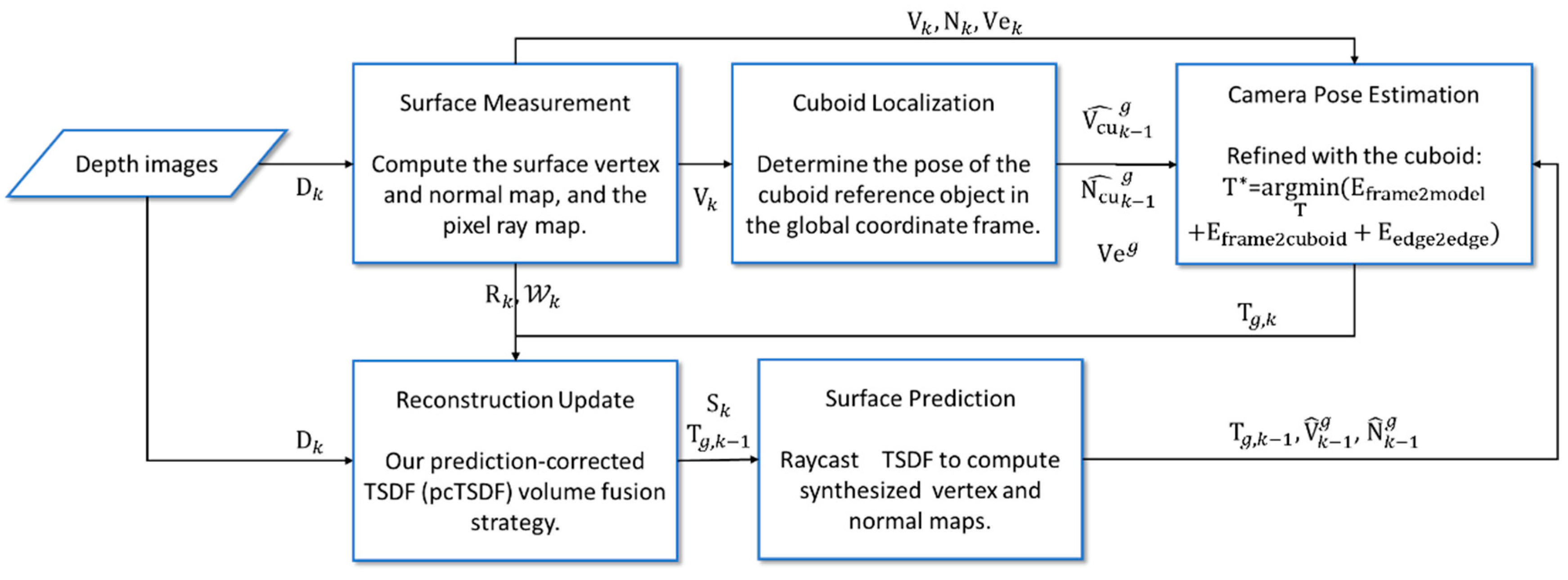
3. Method
3.1. Notation
3.2. Cuboid Localization
3.3. Camera Pose Estimation
3.4. Improved Surface Reconstruction
- are the original TSDF components, and are “ghost” distance value and weight for correction of the existing TSDF prediction;
- and are the view ray and the normal vector in the global coordinate frame respectively, which are used to check if a new surface patch is observed from a different view;
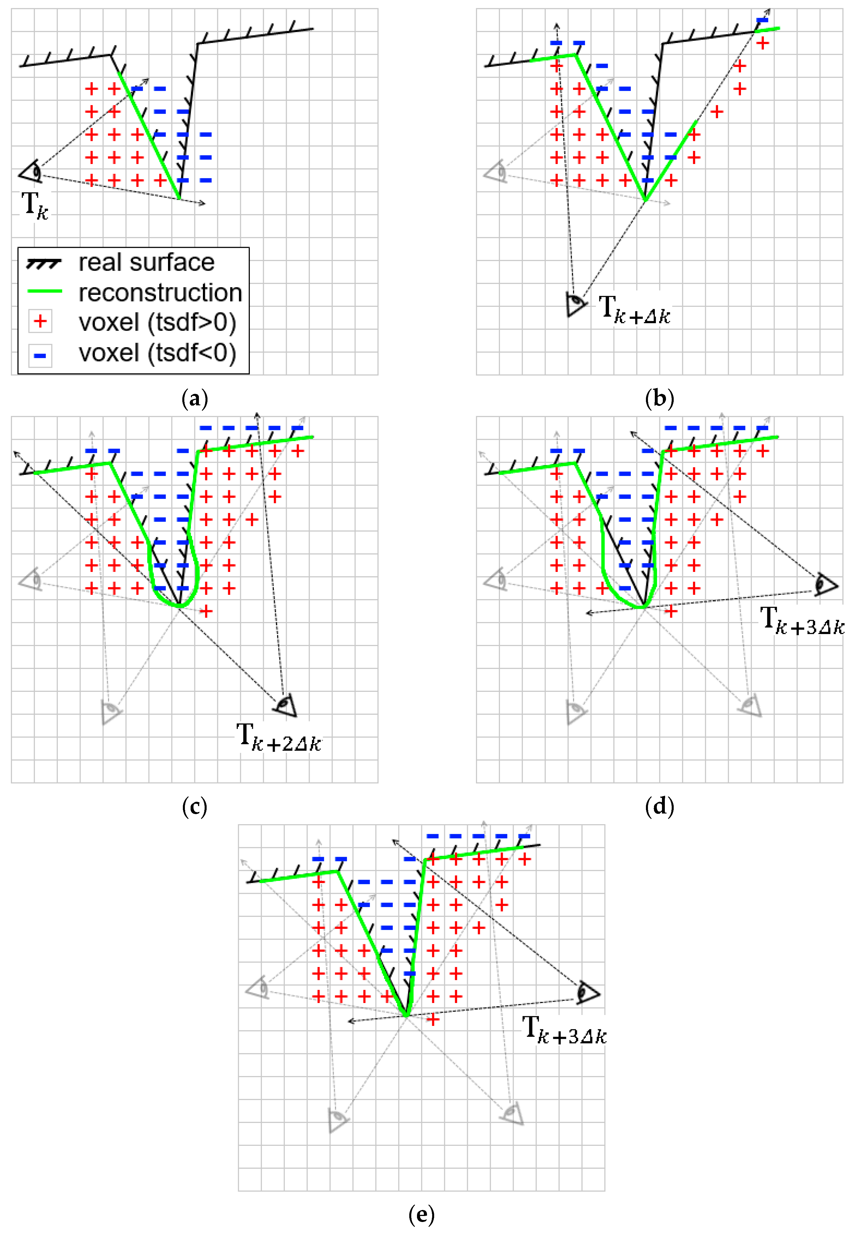
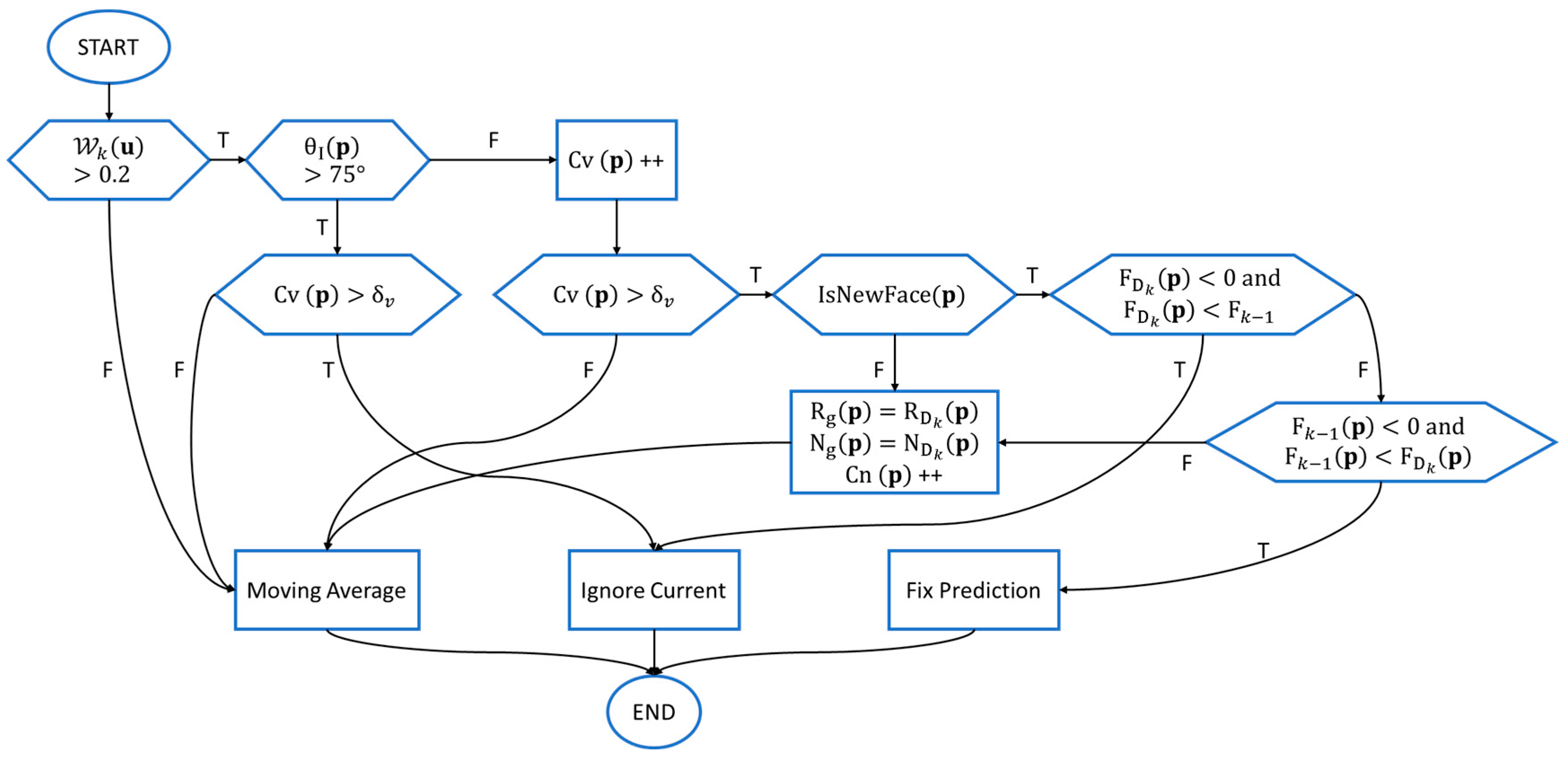
- and are two integer counters as the confidence indices of voxel and its normal vector . When , we think the distance value of voxel has been robustly estimated; when , the normal vector is believed to be stable enough against the measurement noise. A simple Boolean semantic function is defined to check if a new face is observed from a new view point:where the thresholds are set to empirically. We define a weight map for each input frame :with denoting the incidence angle of the view ray to the surface, and is a distance transform map obtained from the contour generator map . For each grid in the TSDF volume, we obtain the adaptive fusion weight and the truncation distance threshold :where is the projection of given the camera pose , and , are the base weight and base truncation distance which are set empirically. Our prediction-corrected TSDF fusion algorithm is then detailed as a flowchart in Figure 7. We categorize the fusion procedure into three sub-strategies:Moving Average: Identical to the TSDF update procedure of KinectFusion, simple moving average TSDF fusion is performed when a voxel has high uncertainty (e.g., at glancing incidence angle or too close to the depth discontinuity edge):Ignore Current: We ignore the TSDF value at the current time when a previously robustly estimated voxel is at glancing incidence angle along the view ray. This is also the case when the current TSDF value with higher uncertainty is observed from a new perspective.Fix Prediction: When a voxel with previously stable TSDF value is observed to increase from a new point of view—either with or —we believe the live TSDF estimation is more trustworthy as a correction of the previous prediction. In the case of measurement noise, we fuse the live estimation into the ghost storage:and replace the global TSDF with the ghost storage when is above a threshold:
4. Evaluation
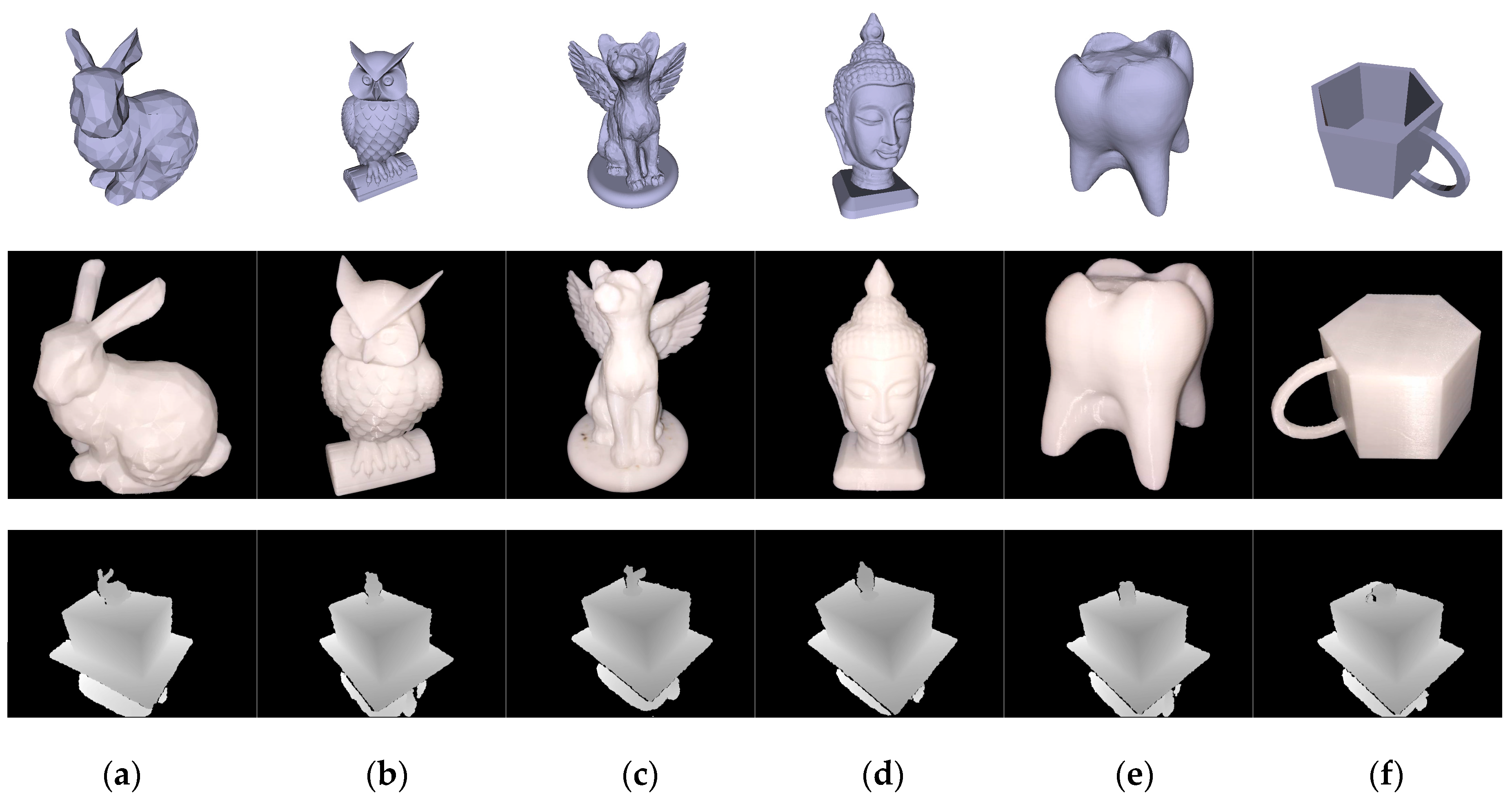
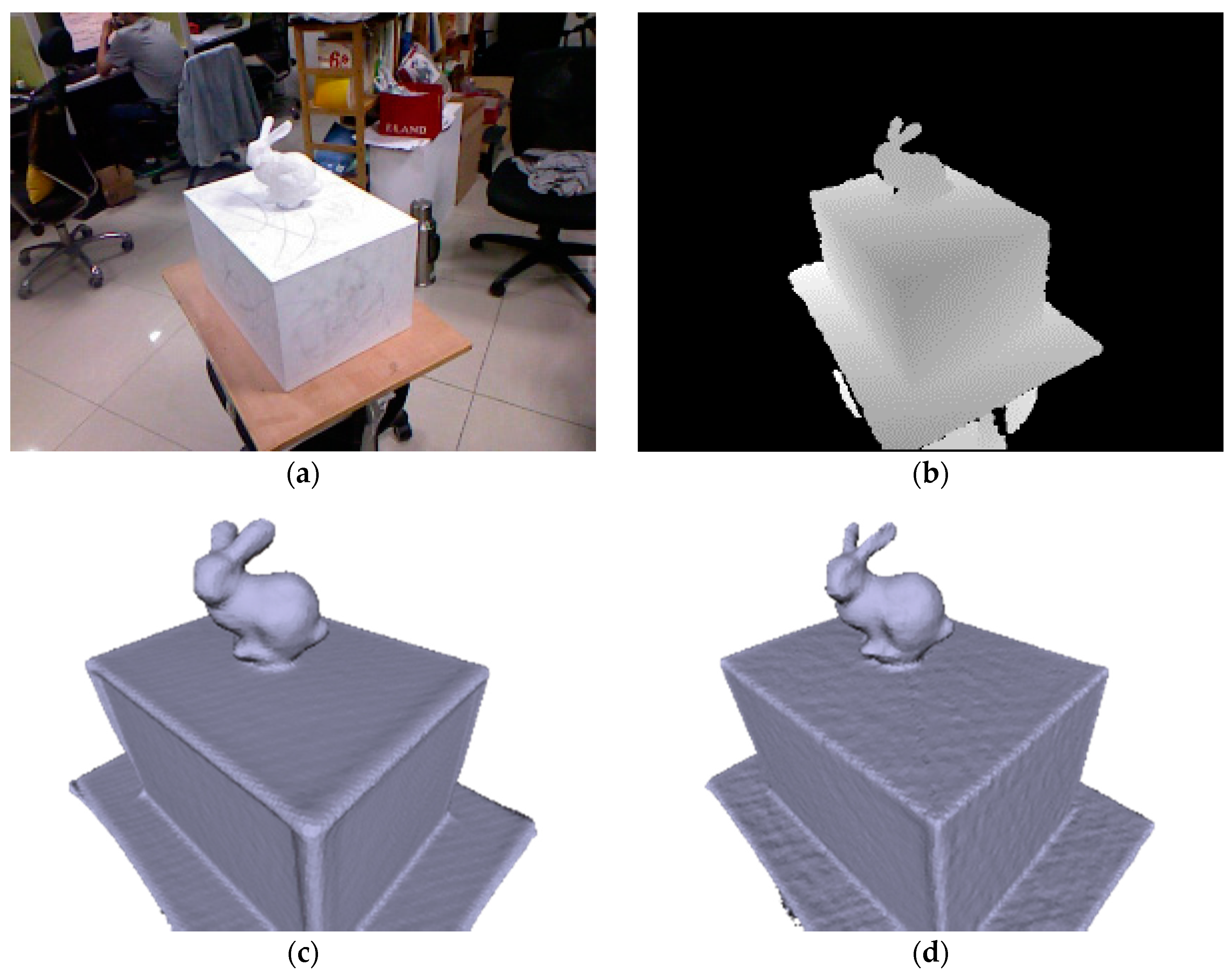
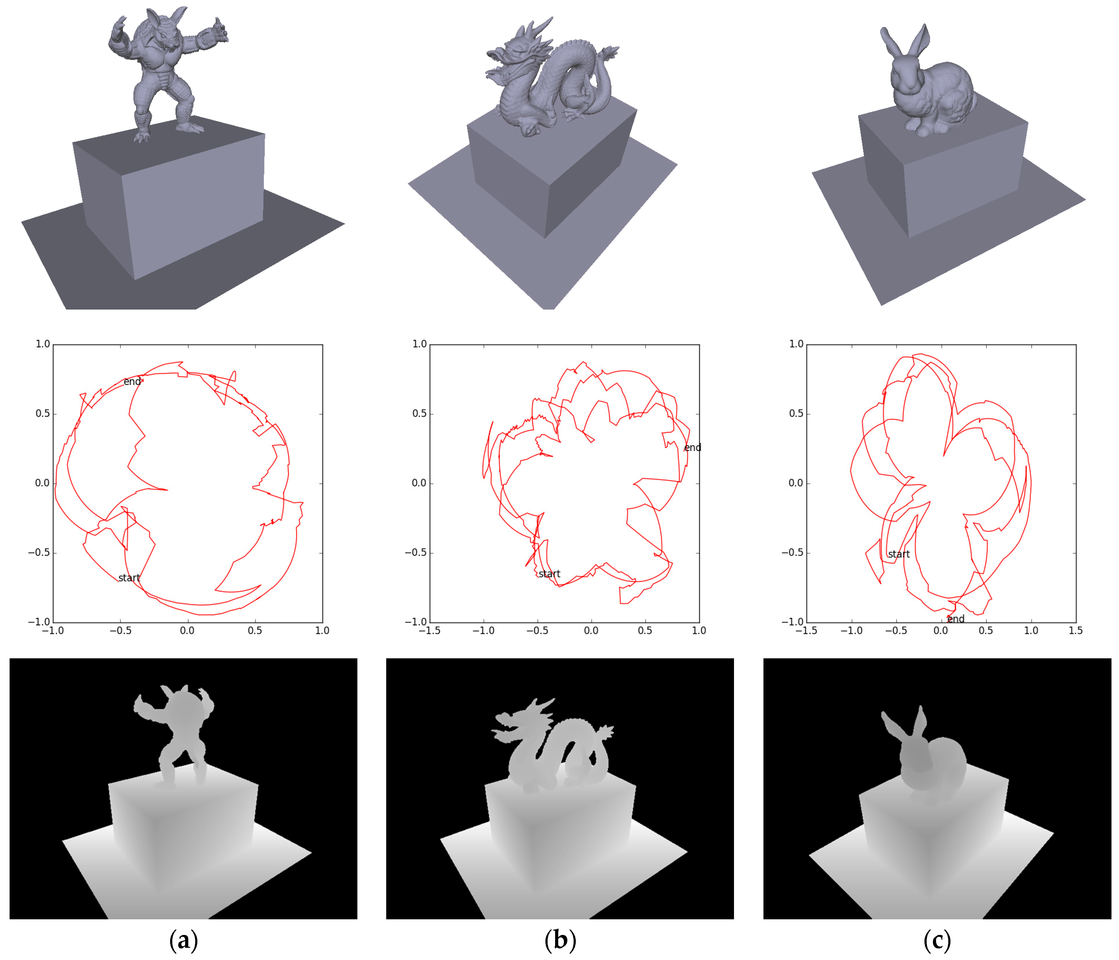
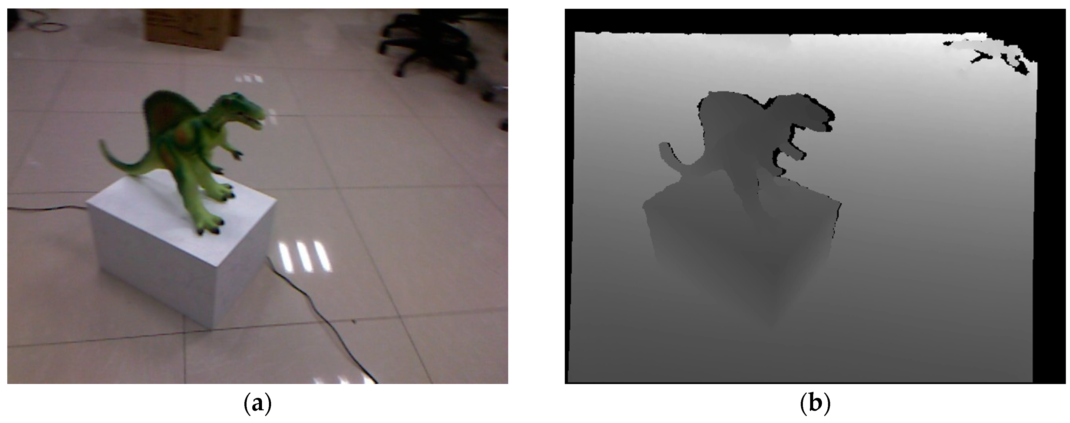
4.1. Dataset
4.2. Error Metrics
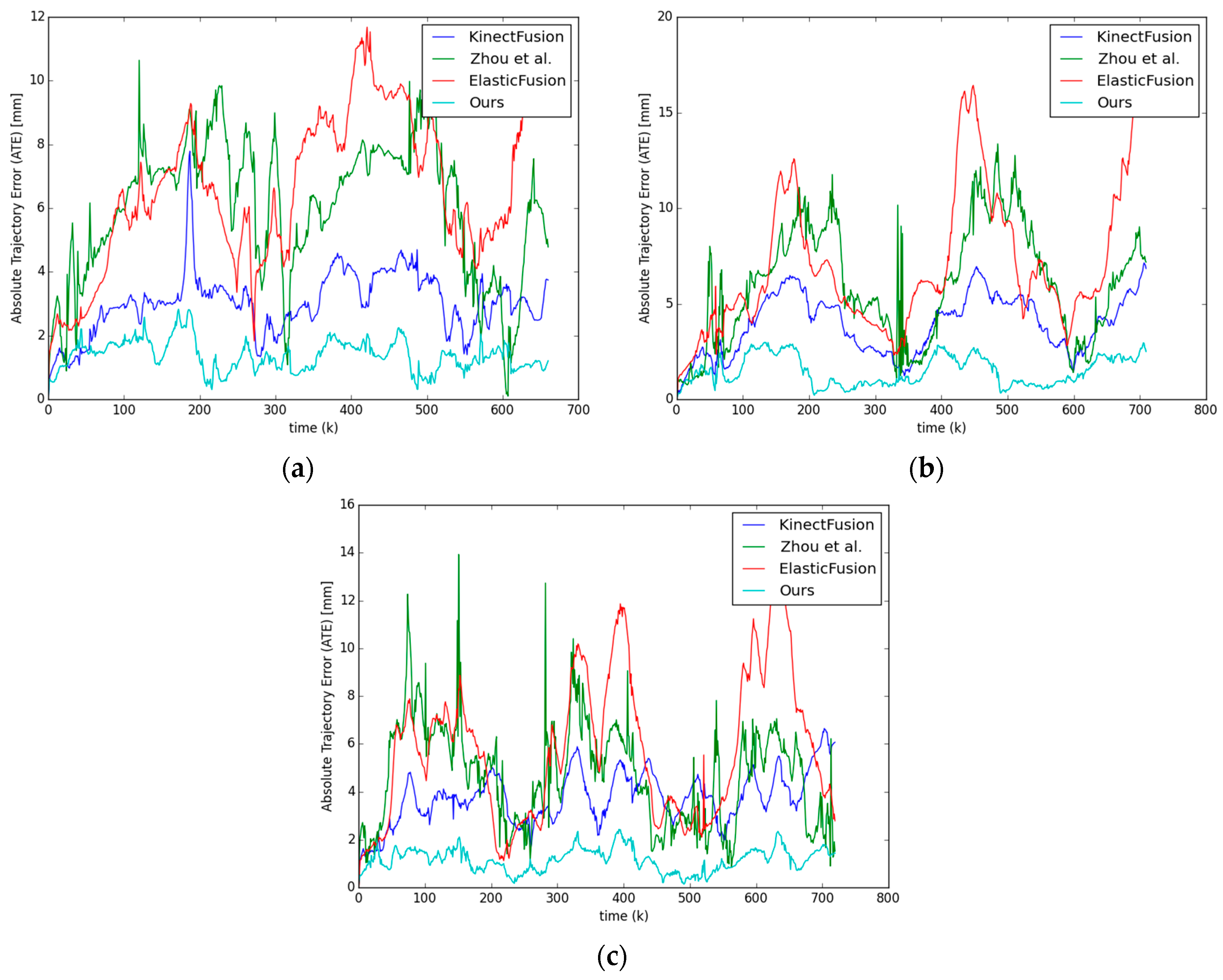
4.3. Camera Trajectory Accuracy
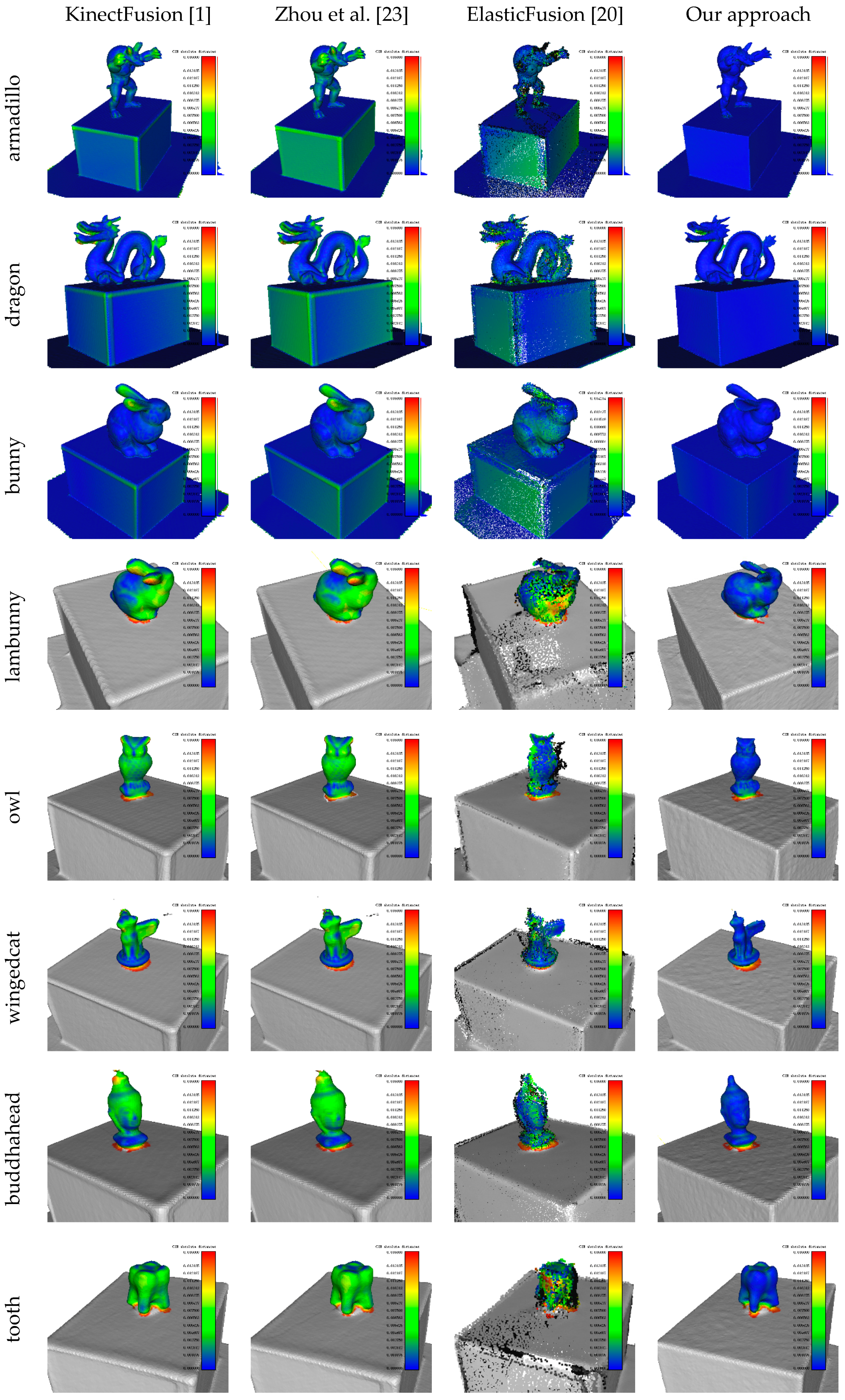
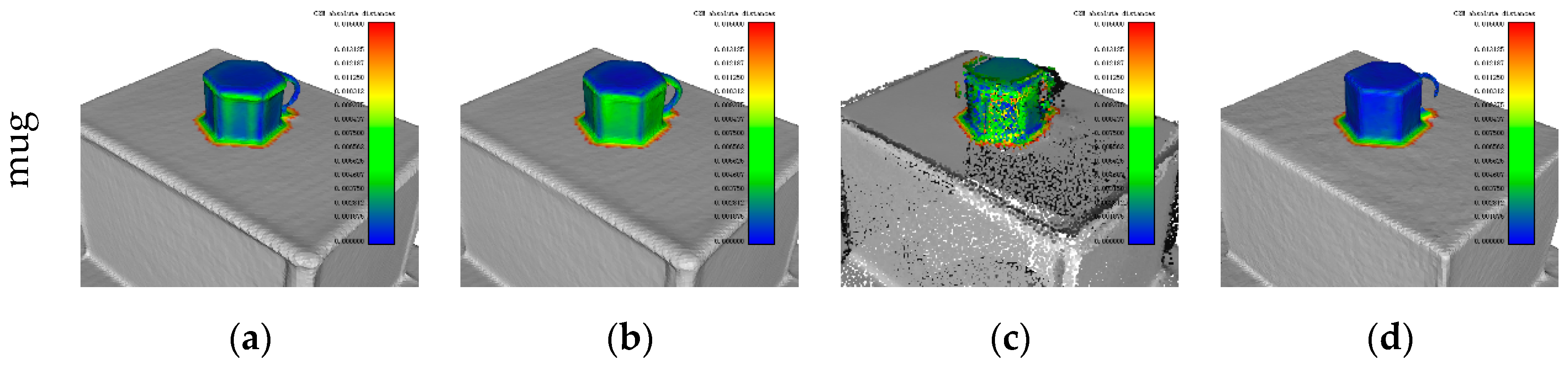
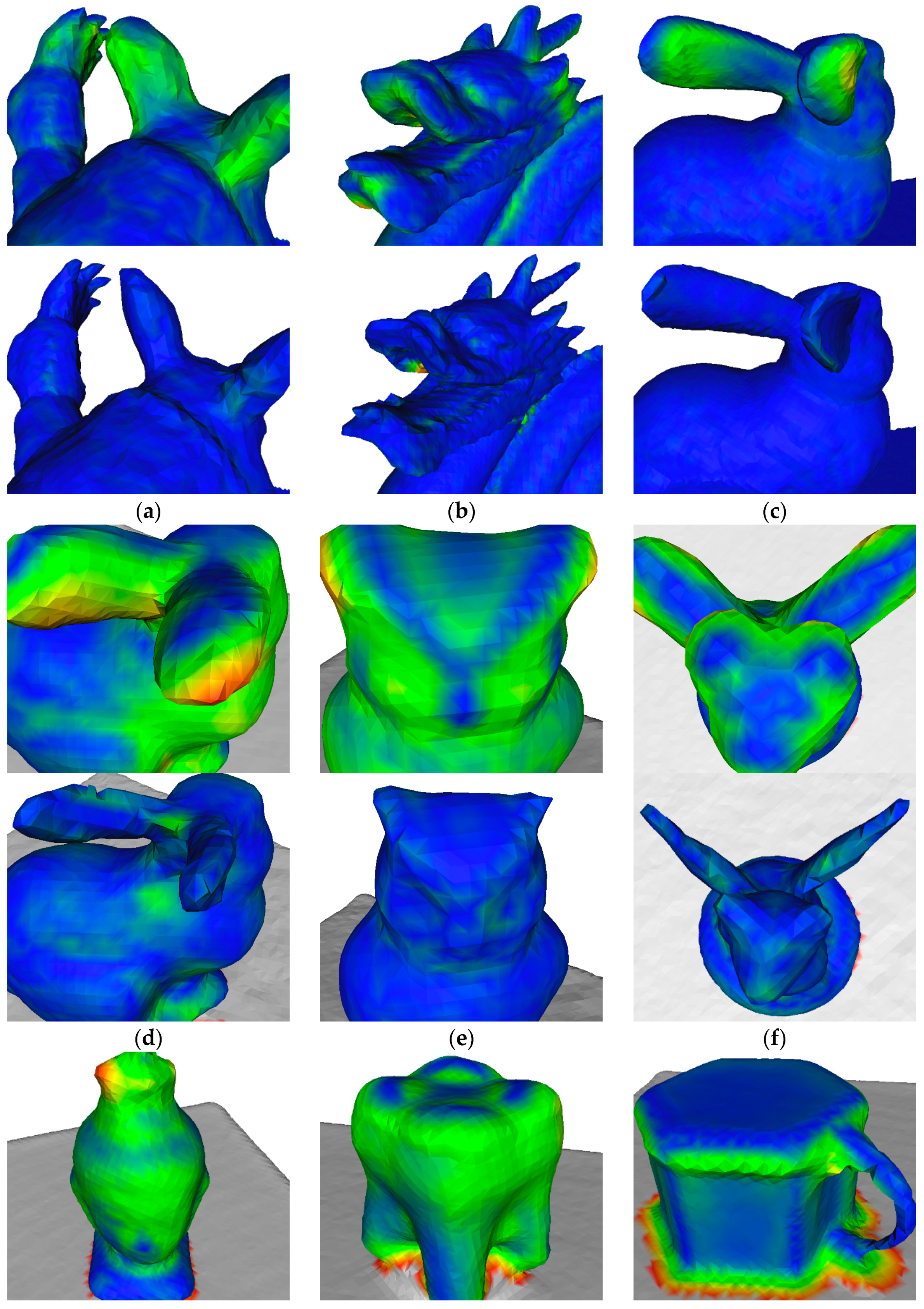
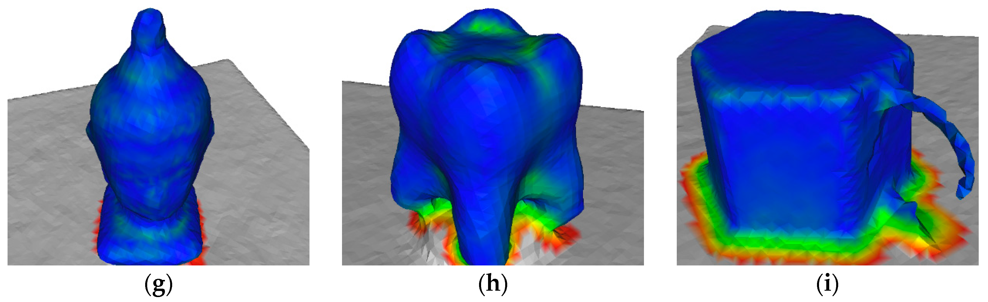
4.4. Surface Reconstruction Accuracy
5. Discussion and Conclusions
Acknowledgments
Author Contributions
Conflicts of Interest
References
- Newcombe, R.A.; Izadi, S.; Hilliges, O.; Molyneaux, D.; Kim, D.; Davison, A.J.; Kohli, P.; Shotton, J.; Hodges, S.; Fitzgibbon, A. KinectFusion: Real-time Dense Surface Mapping and Tracking. In Proceedings of the 2011 10th IEEE International Symposium on Mixed and Augmented Reality (ISMAR ’11), Basel, Switzerland, 26–29 October 2011; IEEE Computer Society: Washington, DC, USA, 2011; pp. 127–136. [Google Scholar]
- Besl, P.J.; McKay, N.D. A method for registration of 3-D shapes. IEEE Trans. Pattern Anal. Mach. Intell. 1992, 14, 239–256. [Google Scholar] [CrossRef]
- Curless, B.; Levoy, M. A Volumetric Method for Building Complex Models from Range Images. In Proceedings of the 23rd Annual Conference on Computer Graphics and Interactive Techniques (SIGGRAPH ’96), New Orleans, LA, USA, 4–9 August 1996; ACM: New York, NY, USA, 1996; pp. 303–312. [Google Scholar]
- Lorensen, W.E.; Cline, H.E. Marching Cubes: A High Resolution 3D Surface Construction Algorithm. In Proceedings of the 14th Annual Conference on Computer Graphics and Interactive Techniques (SIGGRAPH’87), Anaheim, CA, USA, 27–31 July 1987; Volume 21, pp. 163–169. [Google Scholar] [CrossRef]
- Rusinkiewicz, S.; Levoy, M. Efficient variants of the ICP algorithm. In Proceedings of the Third International Conference on 3-D Digital Imaging and Modeling, Quebec City, QC, Canada, 28 May–1 June 2001; pp. 145–152. [Google Scholar]
- Hernandez, C.; Vogiatzis, G.; Cipolla, R. Probabilistic visibility for multi-view stereo. In Proceedings of the 2007 IEEE Conference on Computer Vision and Pattern Recognition, Minneapolis, MN, USA, 17–22 June 2007; pp. 1–8. [Google Scholar]
- Endres, F.; Hess, J.; Sturm, J.; Cremers, D.; Burgard, W. 3-D Mapping with an RGB-D Camera. IEEE Trans. Robot. 2014, 30, 177–187. [Google Scholar] [CrossRef]
- Axelsson, P. Processing of laser scanner data—Algorithms and applications. ISPRS J. Photogramm. Remote Sens. 1999, 54, 138–147. [Google Scholar] [CrossRef]
- Vosselman, G.; Gorte, B.G.; Sithole, G.; Rabbani, T. Recognising structure in laser scanner point clouds. Int. Arch. Photogramm. Remote Sens. Spat. Inf. Sci. 2004, 46, 33–38. [Google Scholar]
- Cui, Y.; Schuon, S.; Chan, D.; Thrun, S.; Theobalt, C. 3D shape scanning with a time-of-flight camera. In Proceedings of the 2010 IEEE Conference on Computer Vision and Pattern Recognition (CVPR), San Francisco, CA, USA, 13–18 June 2010; pp. 1173–1180. [Google Scholar]
- Lange, R.; Seitz, P. Solid-state time-of-flight range camera. IEEE J. Quantum Electron. 2001, 37, 390–397. [Google Scholar] [CrossRef]
- Scharstein, D.; Szeliski, R. High-accuracy stereo depth maps using structured light. In Proceedings of the 2003 IEEE Computer Society Conference on Computer Vision and Pattern Recognition, Madison, WI, USA, 16–22 June 2003; Volume 1, pp. I–195–I–202. [Google Scholar]
- Henry, P.; Krainin, M.; Herbst, E.; Ren, X.; Fox, D. RGB-D mapping: Using Kinect-style depth cameras for dense 3D modeling of indoor environments. Int. J. Robot. Res. 2012, 31, 647–663. [Google Scholar] [CrossRef]
- Segal, A.; Haehnel, D.; Thrun, S. Generalized-ICP. In Proceedings of the Robotics: Science and Systems Conference, Seattle, WA, USA, 28 June–1 July 2009; Volume 2, p. 435. [Google Scholar]
- Nistér, D.; Naroditsky, O.; Bergen, J. Visual odometry. In Proceedings of the 2004 IEEE Computer Society Conference on Computer Vision and Pattern Recognition (CVPR 2004), Washington, DC, USA, 27 June–2 July 2004; Volume 1, pp. I–652–I–659. [Google Scholar]
- Endres, F.; Hess, J.; Engelhard, N.; Sturm, J.; Cremers, D.; Burgard, W. An evaluation of the RGB-D SLAM system. In Proceedings of the 2012 IEEE International Conference on Robotics and Automation (ICRA), St. Paul, MN, USA, 14–18 May 2012; pp. 1691–1696. [Google Scholar]
- Whelan, T.; Kaess, M.; Fallon, M.; Johannsson, H.; Leonard, J.; McDonald, J. Kintinuous: Spatially Extended Kinectfusion. Available online: https://dspace.mit.edu/handle/1721.1/71756 (accessed on 30 September 2017).
- Whelan, T.; Kaess, M.; Johannsson, H.; Fallon, M.; Leonard, J.J.; McDonald, J. Real-time large-scale dense RGB-D SLAM with volumetric fusion. Int. J. Robot. Res. 2015, 34, 598–626. [Google Scholar] [CrossRef]
- Kerl, C.; Sturm, J.; Cremers, D. Dense visual SLAM for RGB-D cameras. In Proceedings of the 2013 IEEE/RSJ International Conference on Intelligent Robots and Systems (IROS), Tokyo, Japan, 3–7 November 2013; pp. 2100–2106. [Google Scholar]
- Whelan, T.; Leutenegger, S.; Moreno, R.S.; Glocker, B.; Davison, A. ElasticFusion: Dense SLAM without A Pose Graph. In Proceedings of the 2015 Robotics: Science and Systems, Rome, Italy, 13–17 July 2015. [Google Scholar]
- Bose, L.; Richards, A. Fast depth edge detection and edge based RGB-D SLAM. In Proceedings of the 2016 IEEE International Conference on Robotics and Automation (ICRA), Stockholm, Sweden, 16–21 May 2016; pp. 1323–1330. [Google Scholar]
- Choi, C.; Trevor, A.J.B.; Christensen, H.I. RGB-D edge detection and edge-based registration. In Proceedings of the 2013 IEEE/RSJ International Conference on Intelligent Robots and Systems, Tokyo, Japan, 3–7 November 2013; pp. 1568–1575. [Google Scholar]
- Zhou, Q.-Y.; Koltun, V. Depth camera tracking with contour cues. In Proceedings of the 2015 IEEE Conference on Computer Vision and Pattern Recognition (CVPR), Boston, MA, USA, 7–12 June 2015; pp. 632–638. [Google Scholar]
- Lefloch, D.; Kluge, M.; Sarbolandi, H.; Weyrich, T.; Kolb, A. Comprehensive Use of Curvature for Robust and Accurate Online Surface Reconstruction. IEEE Trans. Pattern Anal. Mach. Intell. 2017, PP, 1. [Google Scholar] [CrossRef] [PubMed]
- Pumarola, A.; Vakhitov, A.; Agudo, A.; Sanfeliu, A.; Moreno-Noguer, F. PL-SLAM: Real-Time Monocular Visual SLAM with Points and Lines. In Proceedings of the 2017 IEEE International Conference on Robotics and Automation (ICRA), Singapore, 29 May–3 June 2017. [Google Scholar]
- Ma, L.; Kerl, C.; Stückler, J.; Cremers, D. Cpa-slam: Consistent plane-model alignment for direct RGB-D Slam. In Proceedings of the 2016 IEEE International Conference on Robotics and Automation (ICRA), Stockholm, Sweden, 16–21 May 2016; pp. 1285–1291. [Google Scholar]
- Nguyen, T.; Reitmayr, G.; Schmalstieg, D. Structural modeling from depth images. IEEE Trans. Vis. Comput. Graph. 2015, 21, 1230–1240. [Google Scholar] [CrossRef] [PubMed]
- Salas-Moreno, R.F.; Glocken, B.; Kelly, P.H.; Davison, A.J. Dense planar SLAM. In Proceedings of the 2014 IEEE International Symposium on Mixed and Augmented Reality (ISMAR), Munich, Germany, 10–12 September 2014; pp. 157–164. [Google Scholar]
- Taguchi, Y.; Jian, Y.-D.; Ramalingam, S.; Feng, C. Point-plane SLAM for hand-held 3D sensors. In Proceedings of the 2013 IEEE International Conference on Robotics and Automation (ICRA), Karlsruhe, Germany, 6–10 May 2013; pp. 5182–5189. [Google Scholar]
- Hornung, A.; Wurm, K.M.; Bennewitz, M.; Stachniss, C.; Burgard, W. OctoMap: An efficient probabilistic 3D mapping framework based on octrees. Auton. Robots 2013, 34, 189–206. [Google Scholar] [CrossRef]
- Keller, M.; Lefloch, D.; Lambers, M.; Izadi, S.; Weyrich, T.; Kolb, A. Real-time 3D reconstruction in dynamic scenes using point-based fusion. In Proceedings of the 2013 International Conference on 3DTV-Conference, Zurich, Switzerland, 29 June–1 July 2013; pp. 1–8. [Google Scholar]
- Serafin, J.; Grisetti, G. NICP: Dense normal based point cloud registration. In Proceedings of the 2015 IEEE/RSJ International Conference on Intelligent Robots and Systems (IROS), Hamburg, Germany, 28 September–2 October 2015; pp. 742–749. [Google Scholar]
- Rusinkiewicz, S.; Hall-Holt, O.; Levoy, M. Real-time 3D model acquisition. ACM Trans. Graph. 2002, 21, 438–446. [Google Scholar] [CrossRef]
- Weise, T.; Wismer, T.; Leibe, B.; Van Gool, L. In-hand scanning with online loop closure. In Proceedings of the 2009 IEEE 12th International Conference on Computer Vision Workshops (ICCV Workshops), Kyoto, Japan, 27 September–4 October 2009; pp. 1630–1637. [Google Scholar]
- Pfister, H.; Zwicker, M.; Van Baar, J.; Gross, M. Surfels: Surface elements as rendering primitives. In Proceedings of the 27th Annual Conference on Computer Graphics and Interactive Techniques, New Orleans, LA, USA, 23–28 July 2000; pp. 335–342. [Google Scholar]
- Meister, S.; Izadi, S.; Kohli, P.; Hämmerle, M.; Rother, C.; Kondermann, D. When can we use kinectfusion for ground truth acquisition. In Proceedings of the Workshop on Color-Depth Camera Fusion in Robotics, Algarve, Portugal, 7 October 2012; Volume 2. [Google Scholar]
- Rusu, R.B.; Cousins, S. 3D is here: Point Cloud Library (PCL). In Proceedings of the 2011 IEEE International Conference on Robotics and Automation, Shanghai, China, 9–13 May 2011; pp. 1–4. [Google Scholar]
- Feng, C.; Taguchi, Y.; Kamat, V.R. Fast plane extraction in organized point clouds using agglomerative hierarchical clustering. In Proceedings of the 2014 IEEE International Conference on Robotics and Automation (ICRA), Hong Kong, China, 31 May–7 June 2014; pp. 6218–6225. [Google Scholar]
- Khoshelham, K.; Elberink, S.O. Accuracy and resolution of kinect depth data for indoor mapping applications. Sensors 2012, 12, 1437–1454. [Google Scholar] [CrossRef] [PubMed]
- Low, K.-L. Linear Least-Squares Optimization for Point-to-Plane ICP Surface Registration; University of North Carolina: Chapel Hill, NC, USA, 2004; Volume 4. [Google Scholar]
- The Stanford 3D Scanning Repository. Available online: http://graphics.stanford.edu/data/3Dscanrep/ (accessed on 18 July 2017).
- Sturm, J.; Engelhard, N.; Endres, F.; Burgard, W.; Cremers, D. A benchmark for the evaluation of RGB-D SLAM systems. In Proceedings of the 2012 IEEE/RSJ International Conference on Intelligent Robots and Systems (IROS), Vilamoura-Algarve, Portugal, 7–12 October 2012; pp. 573–580. [Google Scholar]
- Handa, A.; Whelan, T.; McDonald, J.B.; Davison, A.J. A Benchmark for RGB-D Visual Odometry, 3D Reconstruction and SLAM. In Proceedings of the IEEE International Conference on Robotics and Automation (ICRA), Hong Kong, China, 31 May–7 June 2014. [Google Scholar]
- CloudCompare—Open Source Project. Available online: http://www.danielgm.net/cc/ (accessed on 19 July 2017).


| Scenario | Intrinsic Matrix | ||||
|---|---|---|---|---|---|
| synthetic | (RGB) | 525.50 | 525.50 | 320.00 | 240.00 |
| real-world | (RGB-D) | 529.22 | 528.98 | 313.77 | 254.10 |
| Synthetic Data | KinectFusion [1] | Zhou et al. [23] | ElasticFusion [20] | NICP [32] | Our Approach |
|---|---|---|---|---|---|
| armadillo | 3.2 | 6.4 | 7.1 | 454.6 | 1.5 |
| dragon | 4.2 | 6.7 | 8.0 | 292.8 | 1.7 |
| bunny | 3.9 | 5.1 | 6.6 | 417.8 | 1.3 |
| Synthetic Data | KinectFusion [1] | Zhou et al. [23] | ElasticFusion [20] | Our Approach |
|---|---|---|---|---|
| armadillo | ||||
| dragon | ||||
| bunny |
| Real-World Data | KinectFusion [1] | Zhou et al. [23] | ElasticFusion [20] | Our Approach |
|---|---|---|---|---|
| lambunny | ||||
| owl | ||||
| wingedcat | ||||
| buddhahead | ||||
| tooth | ||||
| mug |
© 2017 by the authors. Licensee MDPI, Basel, Switzerland. This article is an open access article distributed under the terms and conditions of the Creative Commons Attribution (CC BY) license (http://creativecommons.org/licenses/by/4.0/).
Share and Cite
Zhang, C.; Hu, Y. CuFusion: Accurate Real-Time Camera Tracking and Volumetric Scene Reconstruction with a Cuboid. Sensors 2017, 17, 2260. https://doi.org/10.3390/s17102260
Zhang C, Hu Y. CuFusion: Accurate Real-Time Camera Tracking and Volumetric Scene Reconstruction with a Cuboid. Sensors. 2017; 17(10):2260. https://doi.org/10.3390/s17102260
Chicago/Turabian StyleZhang, Chen, and Yu Hu. 2017. "CuFusion: Accurate Real-Time Camera Tracking and Volumetric Scene Reconstruction with a Cuboid" Sensors 17, no. 10: 2260. https://doi.org/10.3390/s17102260
APA StyleZhang, C., & Hu, Y. (2017). CuFusion: Accurate Real-Time Camera Tracking and Volumetric Scene Reconstruction with a Cuboid. Sensors, 17(10), 2260. https://doi.org/10.3390/s17102260