
Towards an Improved LAI Collection Protocol via Simulated and Field-Based PAR Sensing


Abstract
:
1. Introduction
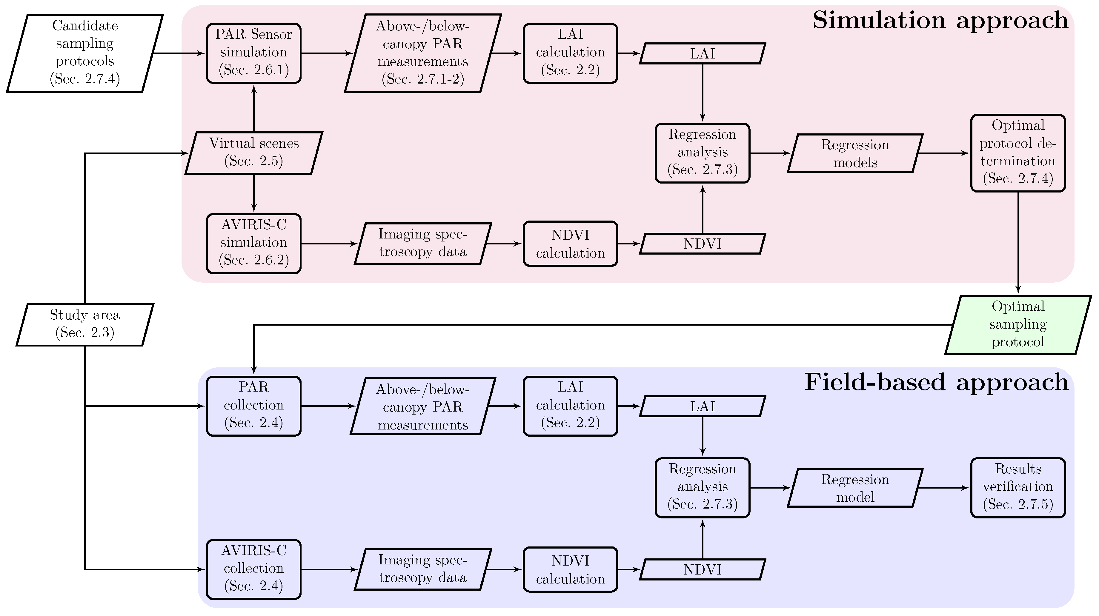
2. Methods
2.1. DIRSIG Background
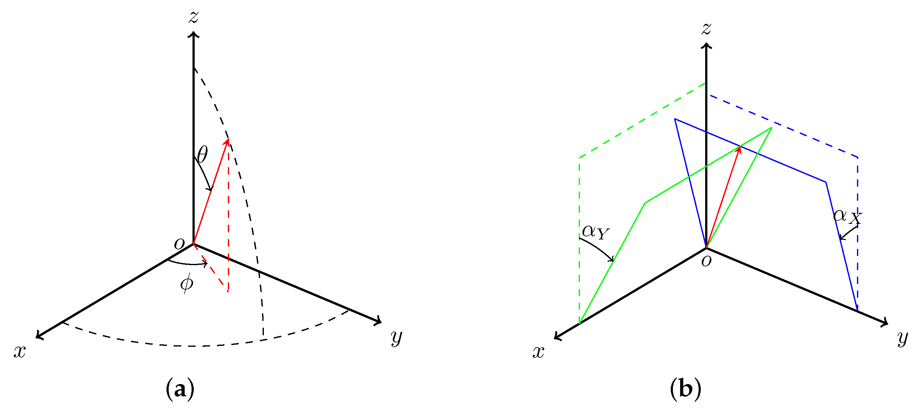
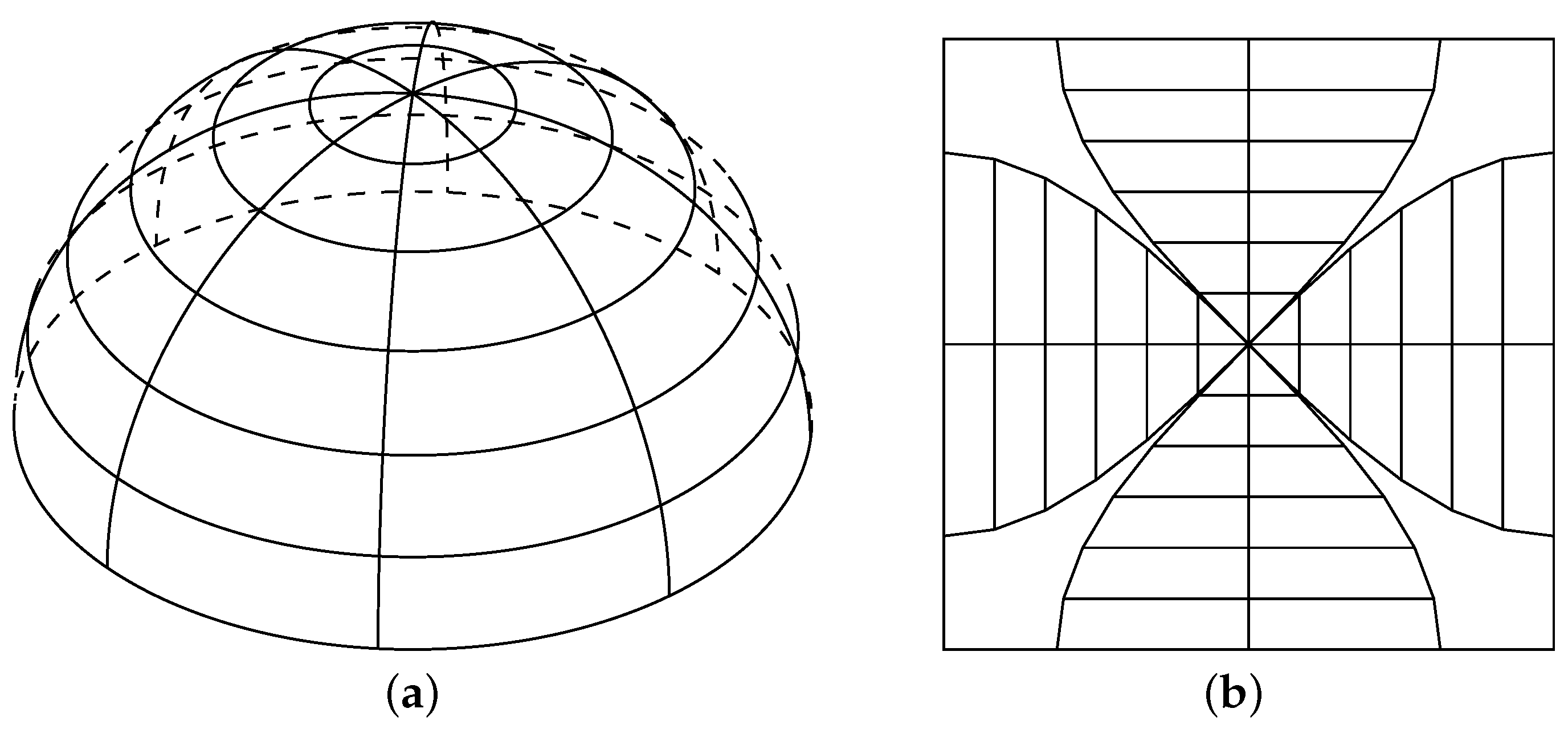
2.2. A Description of the Relevant LAI Theory
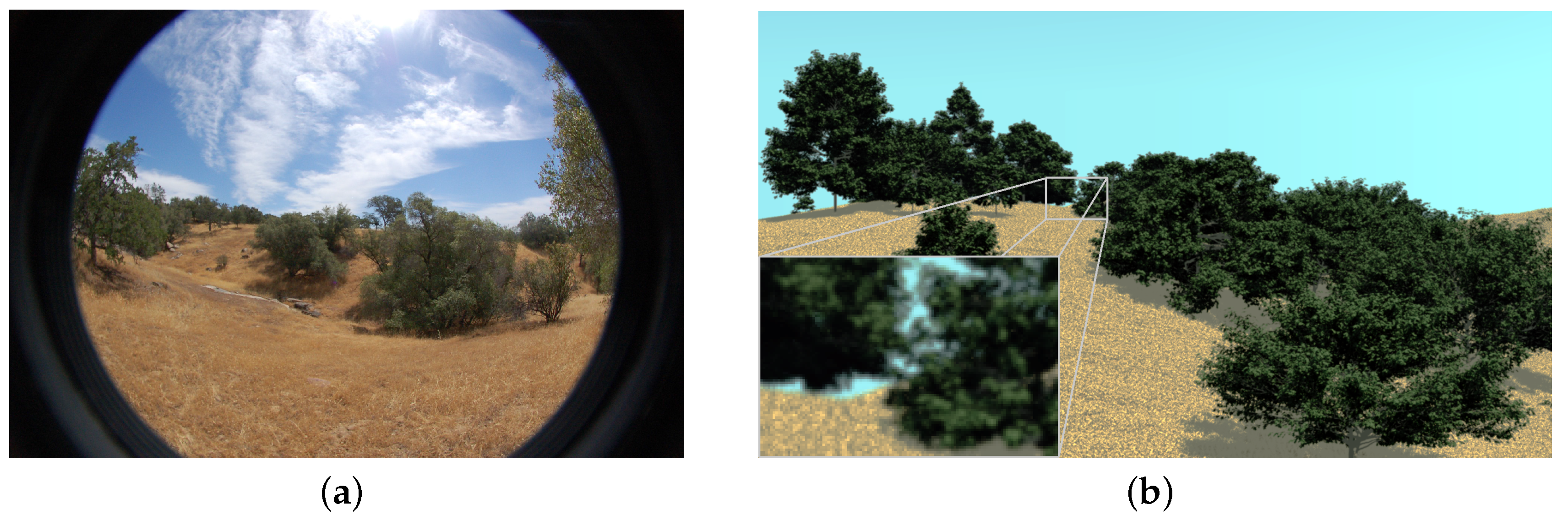
2.3. Study Areas
2.4. Field Inventory and Airborne Imagery Data
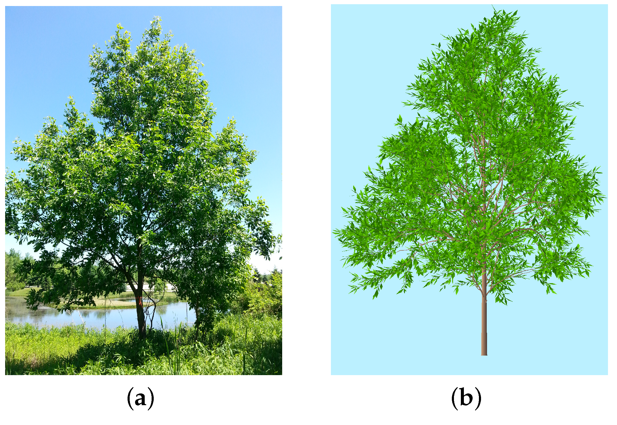
2.5. Virtual Scene Development
2.6. DIRSIG Simulation Design
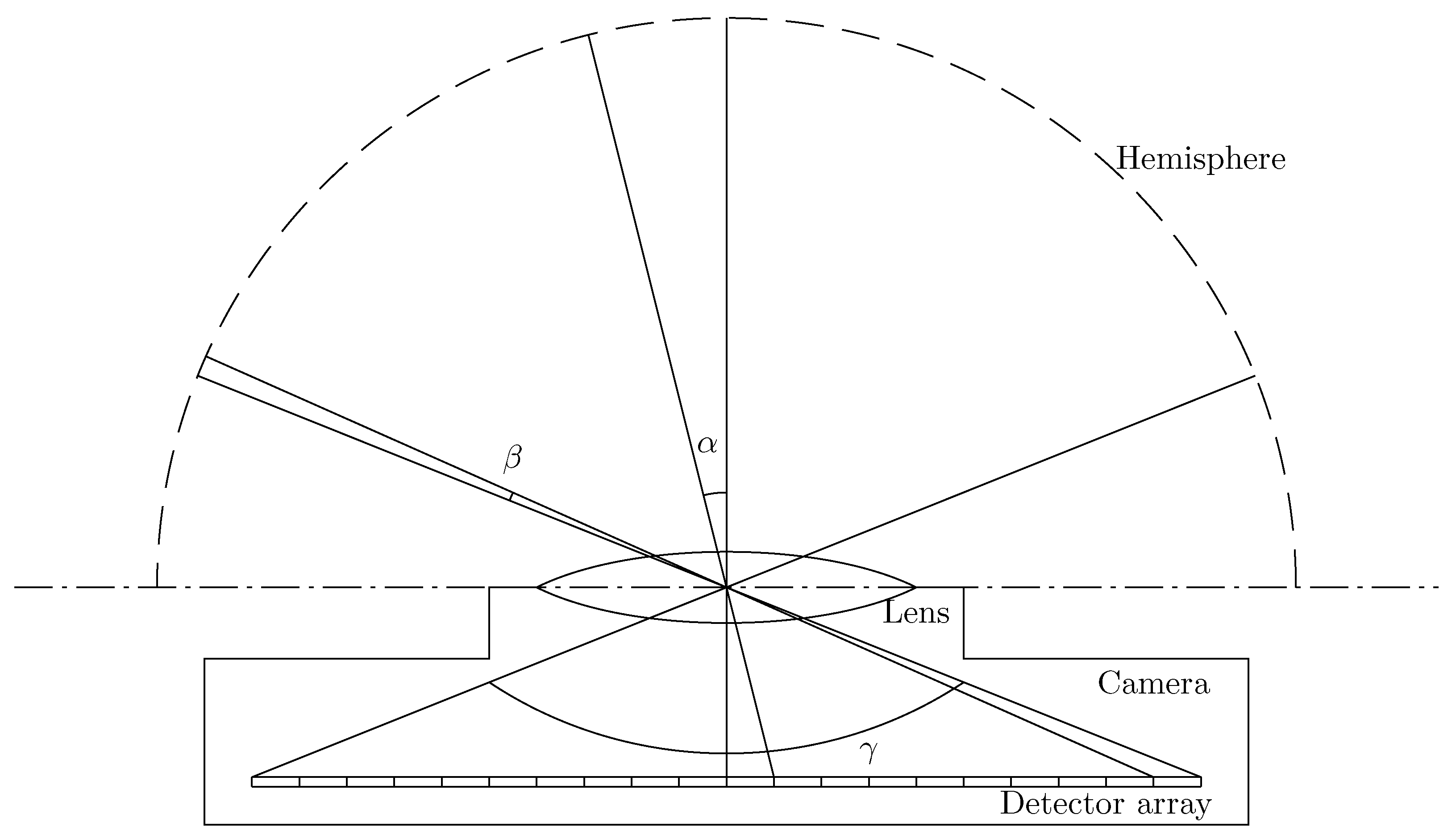
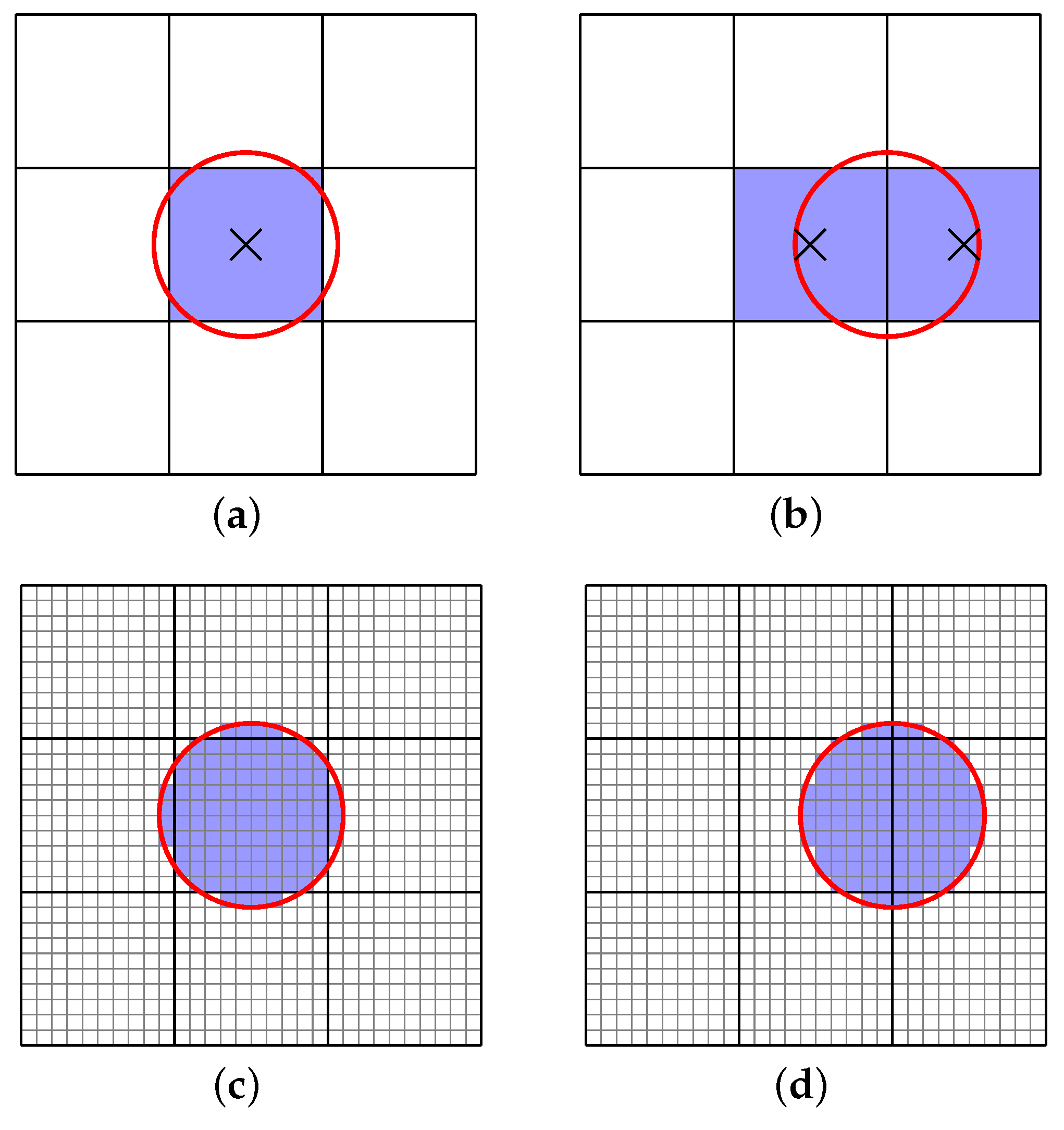
2.6.1. Development of a Simulated PAR Sensor
2.6.2. Simulation of AVIRIS-C Sensor
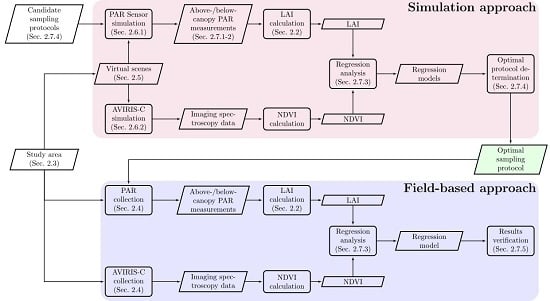
2.7. Experiment Design
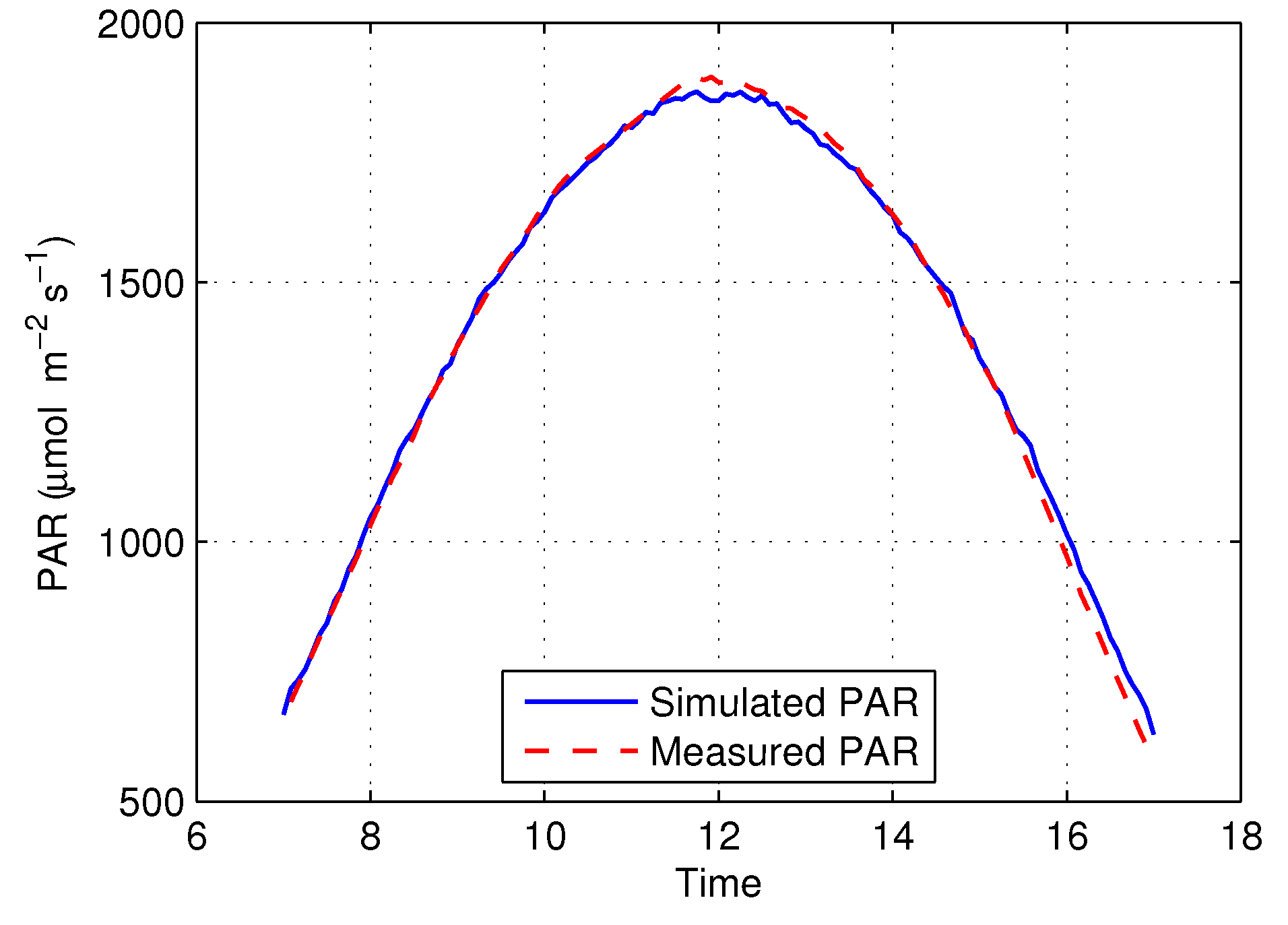
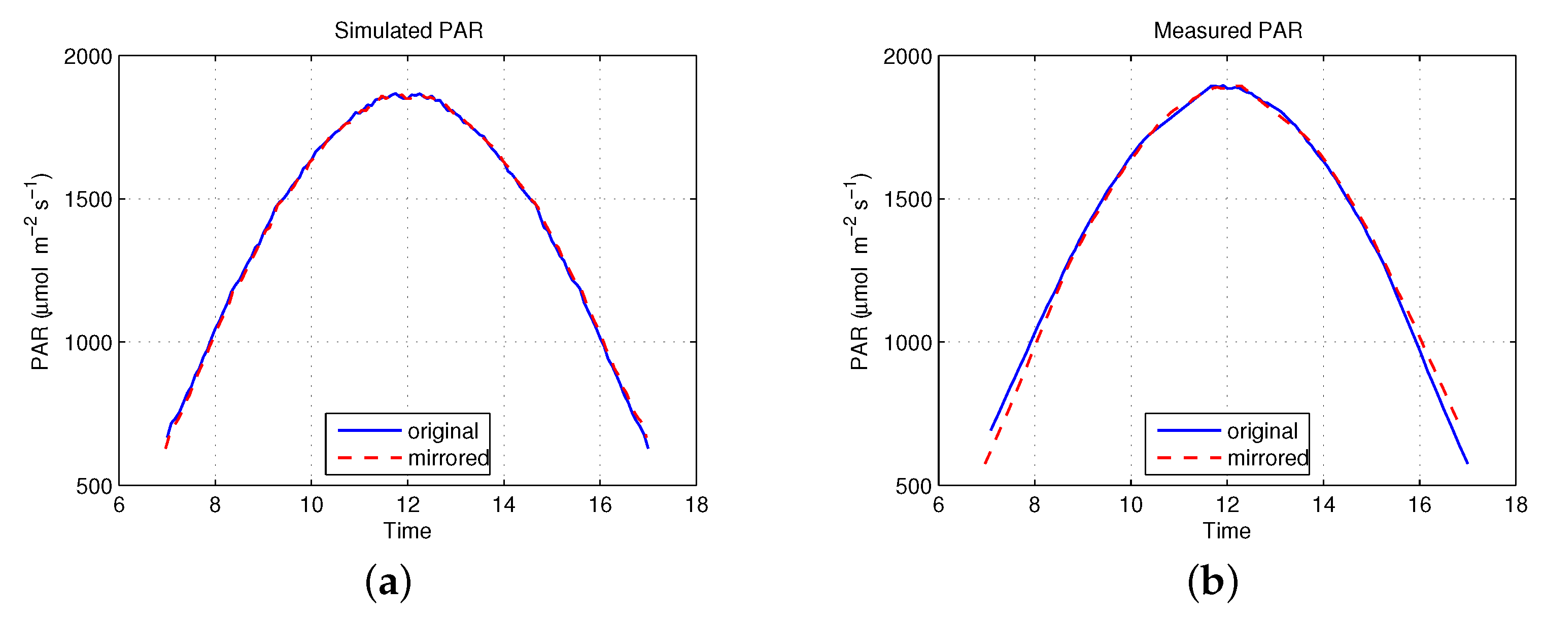
2.7.1. Experiment 1a: Validating Simulated Above-Canopy PAR
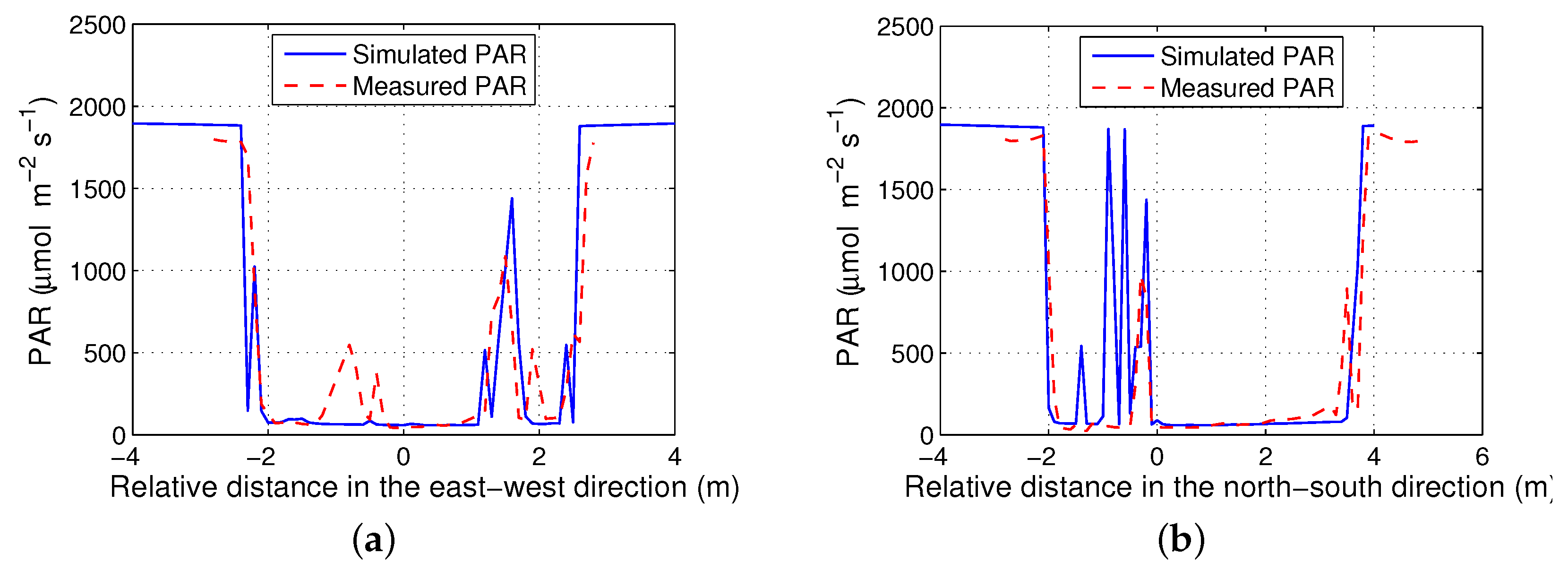
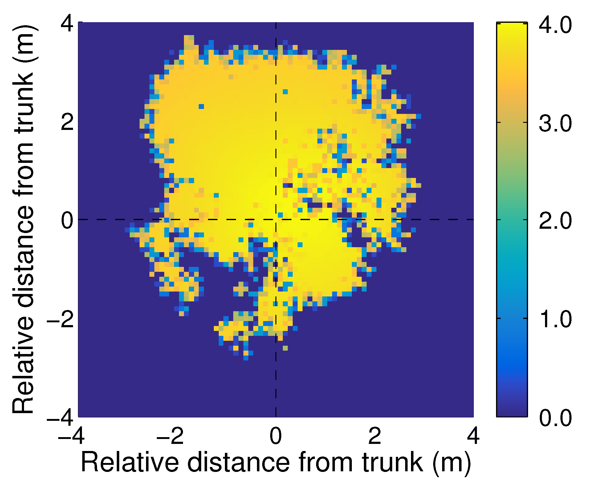
2.7.2. Experiment 1b: Validating Simulated PAR and LAI for a Single Crown
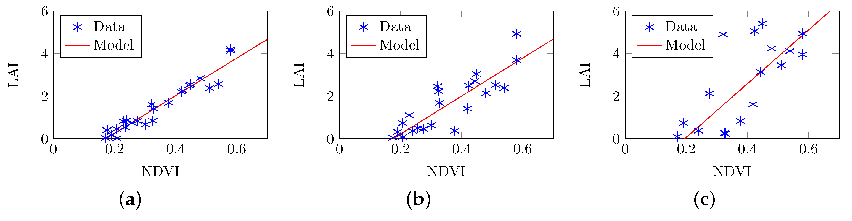
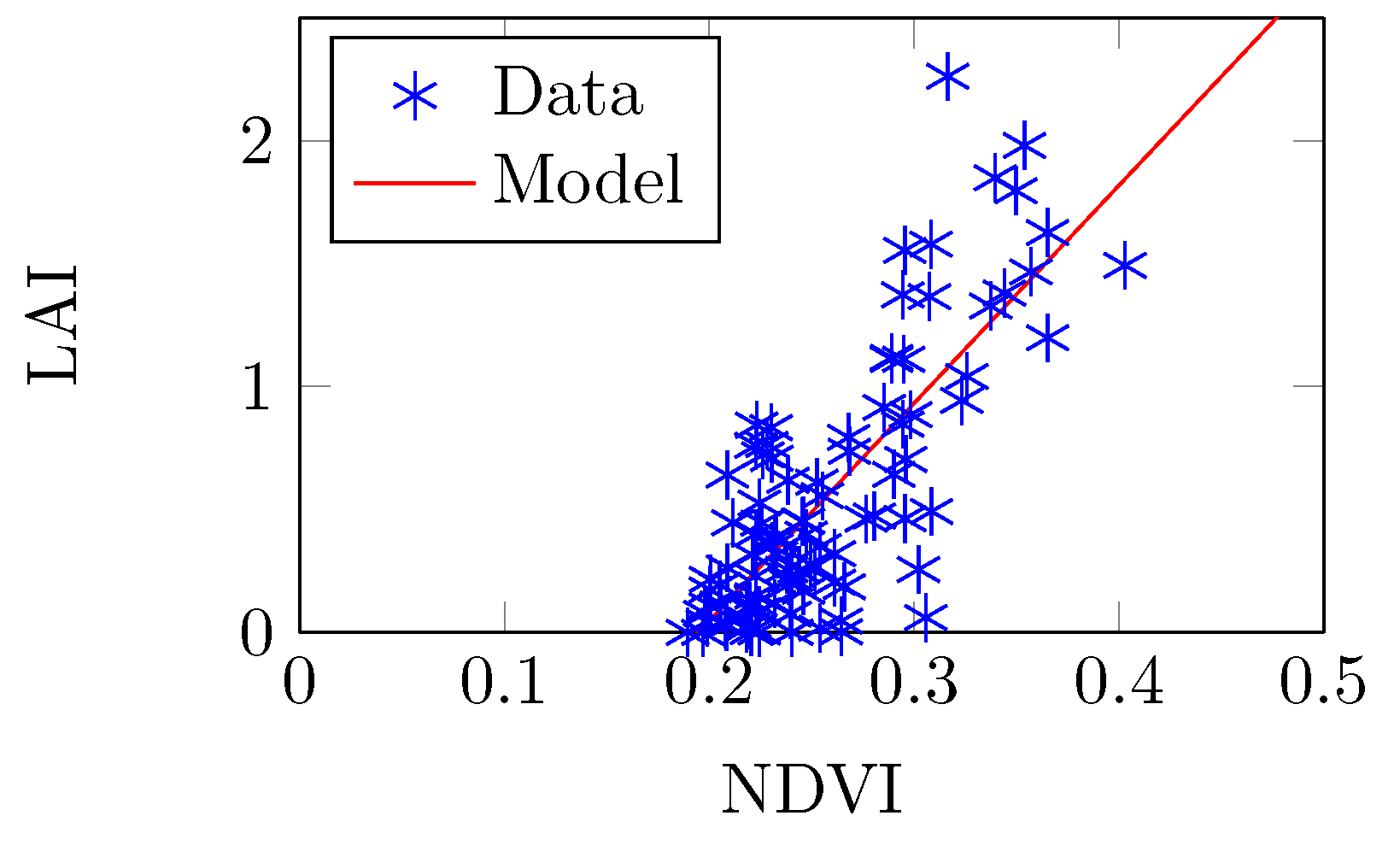
2.7.3. Experiment 1c: Validating Estimated LAI from Simulated PAR for the Forest Site Using Regression to Model NDVI
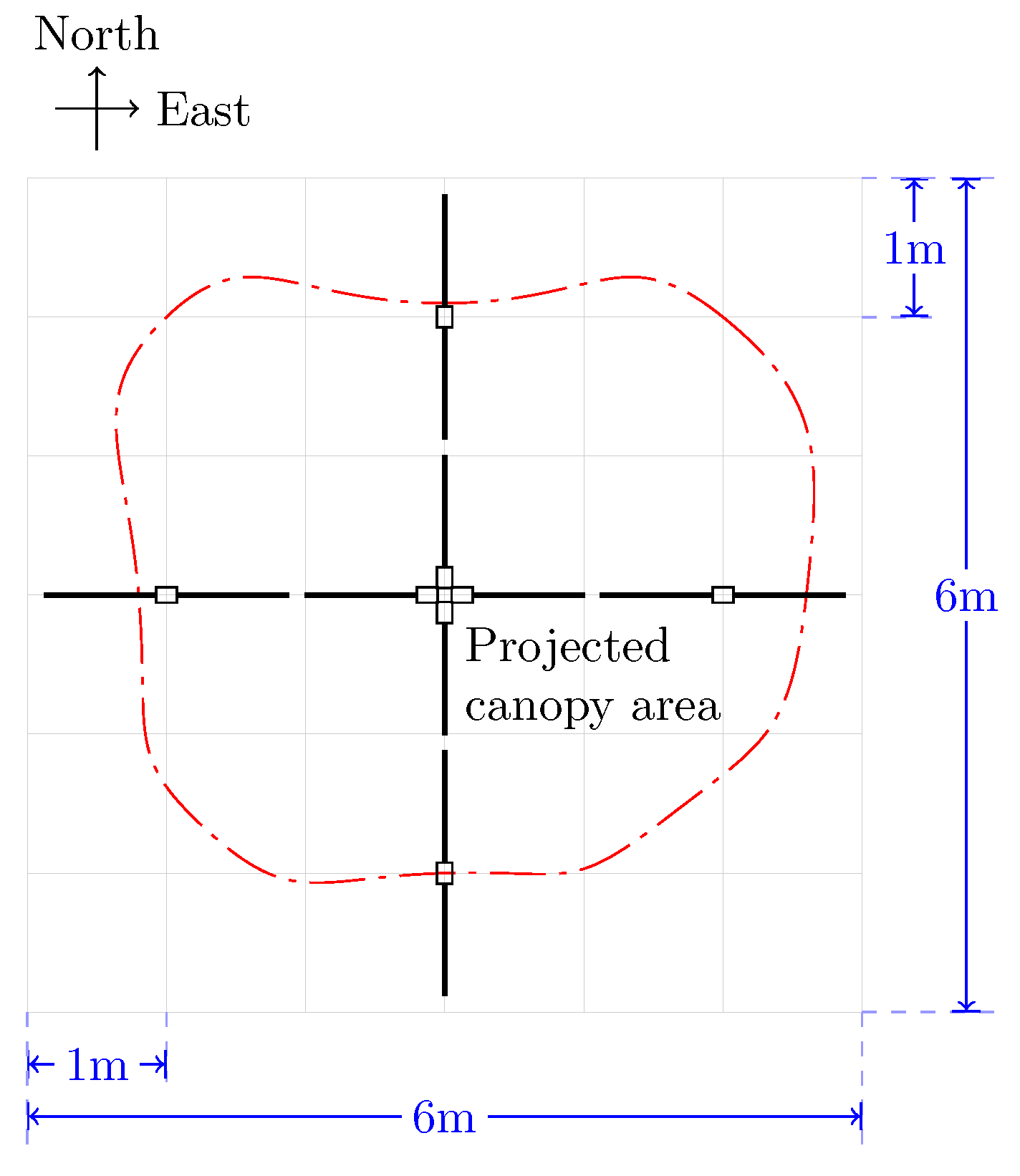
2.7.4. Experiment 2a: Determining Optimal Spacing by Comparing PAR to NDVI for Forest Sites at Various Intervals
2.7.5. Experiment 2b: Comparing in Situ LAI Estimates to NDVI to Verify Simulated Results
3. Results and Discussion
3.1. Experiment 1a: Simulated Above-Canopy PAR
3.2. Experiment 1b: Simulated PAR and LAI for a Single Crown
3.3. Experiment 1c: Estimated LAI from Simulated PAR for the Forest Site Using Regression to Model NDVI
3.4. Experiment 2a: Optimal Spacing by Comparing PAR to NDVI for the Forest Site at Various Intervals
3.5. Experiment 2b: Comparing in Situ LAI Estimates to NDVI to Verify Simulated Results
4. Conclusions
Acknowledgments
Author Contributions
Conflicts of Interest
References
- Hook, S.J.; Turpie, K.; Veraverbeke, S.; Wright, R.; Anderson, M.; Prakash, A.; Mars, J.; Quattrochi, D. NASA 2014 The Hyperspectral Infrared Imager (HyspIRI)—Science Impact of Deploying Instruments on Separate Platforms; Jet Propulsion Laboratory, California Institute of Technology: Pasadena, CA, USA, 2014. [Google Scholar]
- Yao, W.; van Leeuwen, M.; Romanczyk, P.; Kelbe, D.; van Aardt, J. Assessing the impact of sub-pixel vegetation structure on imaging spectroscopy via simulation. Proc. SPIE 2015, 9472, 94721K. [Google Scholar]
- Watson, D.J. Comparative physiological studies on the growth of field crops: I. Variation in net assimilation rate and leaf area between species and varieties, and within and between years. Ann. Bot. 1947, 11, 41–76. [Google Scholar] [CrossRef]
- Chen, J.M.; Black, T.A. Defining leaf area index for non-flat leaves. Plant Cell Environ. 1992, 15, 421–429. [Google Scholar] [CrossRef]
- Lang, A.R.G. Application of some of Cauchy’s theorems to estimation of surface areas of leaves, needles and branches of plants, and light transmittance. Agric. For. Meteorol. 1991, 55, 191–212. [Google Scholar] [CrossRef]
- Running, S.W. A bottom-up evolution of terrestrial ecosystem modeling. In Modeling the Earth System; Ojima, D., Ed.; UCAR/Office for Interdisciplinary Earth Studies: Boulder, CO, USA, 1990; pp. 263–280. [Google Scholar]
- Bonan, G.B. Importance of leaf area index and forest type when estimating photosynthesis in boreal forests. Remote Sens. Environ. 1993, 43, 303–314. [Google Scholar] [CrossRef]
- Bonan, G.B. Land-atmosphere interactions for climate system models: Coupling biophysical, biogeochemical, and ecosystem dynamical processes. Remote Sens. Environ. 1995, 51, 57–73. [Google Scholar] [CrossRef]
- Jonckheere, I.; Fleck, S.; Nackaerts, K.; Muys, B.; Coppin, P.; Weiss, M.; Baret, F. Review of methods for in situ leaf area index determination: Part I. Theories, sensors and hemispherical photography. Agric. For. Meteorol. 2004, 121, 19–35. [Google Scholar] [CrossRef]
- Daughtry, C.S. Direct measurements of canopy structure. Remote Sens. Rev. 1990, 5, 45–60. [Google Scholar] [CrossRef]
- Chen, J.M.; Rich, P.M.; Gower, S.T.; Norman, J.M.; Plummer, S. Leaf area index of boreal forests: Theory, techniques, and measurements. J. Geophys. Res. Atmos. (1984–2012) 1997, 102, 29429–29443. [Google Scholar] [CrossRef]
- Running, S.W.; Nemani, R.R.; Peterson, D.L.; Band, L.E.; Potts, D.F.; Pierce, L.L.; Spanner, M.A. Mapping regional forest evapotranspiration and photosynthesis by coupling satellite data with ecosystem simulation. Ecology 1989, 70, 1090–1101. [Google Scholar] [CrossRef]
- Turner, D.P.; Cohen, W.B.; Kennedy, R.E.; Fassnacht, K.S.; Briggs, J.M. Relationships between leaf area index and Landsat TM spectral vegetation indices across three temperate zone sites. Remote Sens. Environ. 1999, 70, 52–68. [Google Scholar] [CrossRef]
- Verrelst, J.; Rivera, J.P.; Veroustraete, F.; Muñoz-Marí, J.; Clevers, J.G.; Camps-Valls, G.; Moreno, J. Experimental Sentinel-2 LAI estimation using parametric, non-parametric and physical retrieval methods—A comparison. ISPRS J. Photogramm. Remote Sens. 2015, 108, 260–272. [Google Scholar] [CrossRef]
- Novelli, A.; Tarantino, E.; Fratino, U.; Iacobellis, V.; Romano, G.; Gentile, F. A data fusion algorithm based on the Kalman filter to estimate leaf area index evolution in durum wheat by using field measurements and MODIS surface reflectance data. Remote Sens. Lett. 2016, 7, 476–484. [Google Scholar] [CrossRef]
- Weiss, M.; Baret, F.; Smith, G.J.; Jonckheere, I.; Coppin, P. Review of methods for in situ leaf area index (LAI) determination: Part II. Estimation of LAI, errors and sampling. Agric. For. Meteorol. 2004, 121, 37–53. [Google Scholar] [CrossRef]
- AccuPAR PAR/LAI Ceptometer Model LP-80 Operator’s Manual. Available online: http://manuals.decagon.com/Manuals/10242_AccuparLP80_Web.pdf (accessed on 29 February 2015).
- Wilhelm, W.W.; Ruwe, K.; Schlemmer, M.R. Comparison of three leaf area index meters in a corn canopy. Crop Sci. 2000, 40, 1179–1183. [Google Scholar] [CrossRef]
- Facchi, A.; Baroni, G.; Boschetti, M.; Gandolfi, C. Comparing opticaland direct methods for leafarea index determination in a maize crop. J. Agric. Eng. 2010, 41, 33–40. [Google Scholar] [CrossRef]
- Tewolde, H.; Sistani, K.R.; Rowe, D.E.; Adeli, A.; Tsegaye, T. Estimating cotton leaf area index nondestructively with a light sensor. Agron. J. 2005, 97, 1158–1163. [Google Scholar] [CrossRef]
- Johnson, M.V.V.; Kiniry, J.R.; Burson, B.L. Ceptometer deployment method affects measurement of fraction of intercepted photosynthetically active radiation. Agron. J. 2010, 102, 1132–1137. [Google Scholar] [CrossRef]
- Hyer, E.J.; Goetz, S.J. Comparison and sensitivity analysis of instruments and radiometric methods for LAI estimation: Assessments from a boreal forest site. Agric. For. Meteorol. 2004, 122, 157–174. [Google Scholar] [CrossRef]
- Yao, W.; van Leeuwen, M.; Romanczyk, P.; Kelbe, D.; Brown, S.; Kerekes, J.; van Aardt, J. Towards robust forest leaf area index assessment using an imaging spectroscopy simulation approach. In Proceedings of the 2015 IEEE International Geoscience and Remote Sensing Symposium (IGARSS), Milan, Milan, 26–31 July 2015; pp. 5403–5406.
- Avery, T.E.; Burkhart, H.E. Forest Measurements; Waveland Press: Long Grove, IL, USA, 2001. [Google Scholar]
- Schott, J.R.; Brown, S.D.; Raqueno, R.V.; Gross, H.N.; Robinson, G. An advanced synthetic image generation model and its application to multi/hyperspectral algorithm development. Can. J. Remote Sens. 1999, 25, 99–111. [Google Scholar] [CrossRef]
- Schott, J.R.; Raqueno, R.V.; Salvaggio, C. Incorporation of a time-dependent thermodynamic model and a radiation propagation model into IR 3D synthetic image generation. Opt. Eng. 1992, 31, 1505–1516. [Google Scholar] [CrossRef]
- Ientilucci, E.J.; Brown, S.D.; Schott, J.R.; Raqueno, R.V. Multispectral simulation environment for modeling low-light-level sensor systems. In Proceeding of SPIE 3434, Image Intensifiers and Applications; and Characteristics and Consequences of Space Debris and Near-Earth Objects, San Diego, CA, USA, 23 July 1998; International Society for Optics and Photonics (SPIE): Bellingham, WA, USA, 1998; p. 1019. [Google Scholar]
- Gartley, M.; Goodenough, A.; Brown, S.; Kauffman, R.P. A comparison of spatial sampling techniques enabling first principles modeling of a synthetic aperture RADAR imaging platform. Proc. SPIE 2010, 7699, 76990N. [Google Scholar]
- Monsi, M.; Saeki, T. Uber den Lichtfaktor in den Pflanzengesellschaften und seine Bedeutung fur die Stoffproduktion. Jpn. J. Bot. 1953, 14, 22–52. [Google Scholar]
- Monsi, M.; Saeki, T. On the factor light in plant communities and its importance for matter production. Ann. Bot. 2005, 95, 549–567. [Google Scholar] [CrossRef] [PubMed]
- Norman, J.M.; Jarvis, P.G. Photosynthesis in Sitka spruce (Picea sitchensis (Bong.) Carr.): V. Radiation penetration theory and a test case. J. Appl. Ecol. 1975, 12, 839–878. [Google Scholar] [CrossRef]
- Norman, J.M.; Campbell, G.S. Chapter 14: Canopy Structure. In Plant Physiological Ecology: Field Methods and Instrumentation; Pearcey, R., Mooney, H.A., Rundel, P., Eds.; Springer: Dordrecht, The Netherlands, 1989; pp. 301–325. [Google Scholar]
- Campbell, G.S. Extinction coefficients for radiation in plant canopies calculated using an ellipsoidal inclination angle distribution. Agric. For. Meteorol. 1986, 36, 317–321. [Google Scholar] [CrossRef]
- Kampe, T.U.; Johnson, B.R.; Kuester, M.; Keller, M. NEON: The first continental-scale ecological observatory with airborne remote sensing of vegetation canopy biochemistry and structure. J. Appl. Remote Sens. 2010, 4, 043510. [Google Scholar] [CrossRef]
- Kampe, T.; Leisso, N.; Musinsky, J.; Petroy, S.; Karpowicz, B.; Krause, K.; Crocker, R.I.; DeVoe, M.; Penniman, E.; Guadagno, T.; et al. TM-005: The NEON 2013 Airborne Campaign at Domain 17 Terrestrial and Aquatic Sites in California. 2013. Available online: http://www.neoninc.org/data-resources/papers-publications/ (accessed on 15 March 2016).
- Onyx Computing, Inc. OnyxTREE [Software]. 1992–2011. Available online: http://www.onyxtree.com (accessed on 1 June 2016).
- Jones, B.W. Discovering the Solar System, 2nd ed.; Wiley: Hoboken, NJ, USA, 2007. [Google Scholar]
- Reda, I.; Andreas, A. Solar position algorithm for solar radiation applications. Sol. Energy 2004, 76, 577–589. [Google Scholar] [CrossRef]
- Berk, A.; Anderson, G.P.; Bernstein, L.S.; Acharya, P.K.; Dothe, H.; Matthew, M.W.; Adler-Golden, S.M.; Chetwynd, J.H., Jr.; Richtsmeier, S.C.; Pukall, B.; et al. MODTRAN4 radiative transfer modeling for atmospheric correction. Proc. SPIE 1999, 3756, 348. [Google Scholar]
- Richardson, A.J.; Weigand, C.L. Distinguishing vegetation from soil background information. Photogramm. Eng. Remote Sens. 1977, 43, 1541–1552. [Google Scholar]
- Gong, P.; Pu, R.; Biging, G.S.; Larrieu, M.R. Estimation of forest leaf area index using vegetation indices derived from Hyperion hyperspectral data. IEEE Trans. Geosci. Remote Sens. 2003, 41, 1355–1362. [Google Scholar] [CrossRef]
- Lüdeke, M.; Janecek, A.; Kohlmaier, G.H. Modelling the seasonal CO2 uptake by land vegetation using the global vegetation index. Tellus B 2002, 43, 188–196. [Google Scholar] [CrossRef]
- Wang, Q.; Adiku, S.; Tenhunen, J.; Granier, A. On the relationship of NDVI with leaf area index in a deciduous forest site. Remote Sens. Environ. 2005, 94, 244–255. [Google Scholar] [CrossRef]
- Kleinbaum, D.G.; Kupper, L.L. Applied Regression Analysis and Other Multivariable Methods; Duxbury Press: Pacific Grove, CA, USA, 1978. [Google Scholar]
- Pagano, M.; Gauvreau, K. Principles of Biostatistics, 2nd ed.; Duxbury Press: Pacific Grove, CA, USA, 2000. [Google Scholar]
- Oberkampf, W.L.; DeLand, S.M.; Rutherford, B.M.; Diegert, K.V.; Alvin, K.F. Error and uncertainty in modeling and simulation. Reliab. Eng. Syst. Saf. 2002, 75, 333–357. [Google Scholar] [CrossRef]


| Parameter | Value (Unit) |
|---|---|
| Height | 7.4 (m) |
| Crown width (in West-East direction) | 4.8 (m) |
| Crown width (in South-North direction) | 4.1 (m) |
| DBH (at the first branch, 1.2 m from ground) | 18 (cm) |
| LAI | 3.5 |
| ID | Type | Height | Crown Dia. | Instance 1 | Instance 2 | Instance 3 | |||
|---|---|---|---|---|---|---|---|---|---|
| x | y | x | y | x | y | ||||
| 1 | Broadleaf | 9.78 | 17.34 | 2.96 | −15.16 | – | – | – | – |
| 2 | Broadleaf | 10.87 | 11.82 | 5.76 | −2.86 | – | – | – | – |
| 3-1 | Conifer | 13.16 | 12.66 | −7.67 | −9.15 | – | – | – | – |
| 3-2 | Conifer | 15.15 | 10.57 | −1.81 | −7.25 | – | – | – | – |
| 4 | Broadleaf | 5.97 | 4.15 | −13.14 | 2.44 | 8.16 | 6.64 | 8.36 | 13.44 |
| 5-1 | Broadleaf | 6.44 | 10.14 | −4.04 | 19.14 | – | – | – | – |
| 5-2 | Broadleaf | 8.47 | 11.35 | 0.96 | 14.64 | – | – | – | – |
| 6-1 | Broadleaf | 10.77 | 18.27 | 17.06 | 9.14 | 39.86 | −37.14 | – | – |
| 6-2 | Broadleaf | 9.05 | 16.39 | 17.26 | 3.14 | 13.26 | 3.14 | 9.14 | −42.28 |
| 7 | Conifer | 15.07 | 14.27 | −24.64 | −8.01 | – | – | – | – |
| 8 | Broadleaf | 14.12 | 13.64 | −27.03 | 4.77 | – | – | – | – |
| 9 | Broadleaf | 8.94 | 8.04 | −10.36 | −36.14 | −12.57 | −40.43 | – | – |
| 10 | Broadleaf | 8.27 | 12.94 | −37.85 | −27.50 | – | – | – | – |
| 11 | Broadleaf | 11.76 | 20.80 | 22.03 | −12.72 | – | – | – | – |
| 12 | Broadleaf | 9.41 | 14.40 | 29.52 | −27.52 | – | – | – | – |
| 13 | Broadleaf | 12.05 | 17.81 | 39.08 | 10.37 | – | – | – | – |
| 14 | Broadleaf | 9.90 | 16.17 | 27.08 | 35.93 | – | – | – | – |
| 15 | Broadleaf | 7.65 | 9.93 | −0.61 | 34.50 | −41.71 | 16.43 | – | – |
| 16 | Broadleaf | 8.06 | 12.11 | −22.58 | 15.23 | – | – | – | – |
| 17-1 | Broadleaf | 8.78 | 10.01 | −29.84 | 28.82 | – | – | – | – |
| 17-2 | Broadleaf | 7.12 | 7.91 | −28.71 | 22.43 | – | – | – | – |
| 18 | Conifer | 12.33 | 6.84 | −16.50 | 26.40 | – | – | – | – |
| 19 | Broadleaf | 9.65 | 10.25 | −14.13 | 33.29 | −13.06 | 39.82 | – | – |
| 20 | Broadleaf | 15.64 | 10.65 | −21.79 | 39.31 | – | – | – | – |
| 21 | Broadleaf | 5.98 | 3.95 | −39.43 | 39.86 | −39.16 | −21.52 | −19.78 | 1.09 |
| 22 | Broadleaf | 5.96 | 5.47 | −35.29 | 0.43 | – | – | – | – |
| Parameter | Value (Unit) |
|---|---|
| Scan rate | 12 (Hz) |
| IFOV | 0.8 (m rad) |
| Number of bands | 224 |
| Spectral range | 380–2500 (nm) |
| Spectral sampling | 10 (nm) |
| Spectral response | Gaussian, FWHM = 10 (nm) |
| Flight altitude | 18.5 (km) |
| Flight speed | 177.6 (m/s) |
| Interval | Number of Measurements | Number of Measurements |
|---|---|---|
| in an Plot | in a Square | |
| 5 m | 1360 | 45 |
| 10 m | 720 | 30 |
| 15 m | 400 | 15 |
| Pair | Slope | Intercept | |||
|---|---|---|---|---|---|
| Model 1 | Model 2 | Test Statistic (T) | Probability (p) | Test Statistic (T) | Probability (p) |
| 5 m-interval | 10 m-interval | −0.091 | 0.928 | 0.148 | 0.883 |
| 5 m-interval | 15 m-interval | −1.936 | 0.059 | 1.343 | 0.186 |
© 2016 by the authors; licensee MDPI, Basel, Switzerland. This article is an open access article distributed under the terms and conditions of the Creative Commons Attribution (CC-BY) license (http://creativecommons.org/licenses/by/4.0/).
Share and Cite
Yao, W.; Kelbe, D.; Leeuwen, M.V.; Romanczyk, P.; Aardt, J.V. Towards an Improved LAI Collection Protocol via Simulated and Field-Based PAR Sensing. Sensors 2016, 16, 1092. https://doi.org/10.3390/s16071092
Yao W, Kelbe D, Leeuwen MV, Romanczyk P, Aardt JV. Towards an Improved LAI Collection Protocol via Simulated and Field-Based PAR Sensing. Sensors. 2016; 16(7):1092. https://doi.org/10.3390/s16071092
Chicago/Turabian StyleYao, Wei, David Kelbe, Martin Van Leeuwen, Paul Romanczyk, and Jan Van Aardt. 2016. "Towards an Improved LAI Collection Protocol via Simulated and Field-Based PAR Sensing" Sensors 16, no. 7: 1092. https://doi.org/10.3390/s16071092