
Automatic Censoring CFAR Detector Based on Ordered Data Difference for Low-Flying Helicopter Safety


Abstract
:1. Introduction
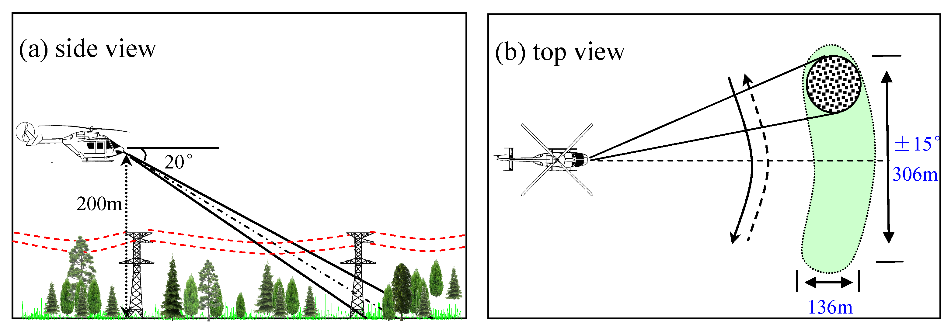
2. Target Detection Model of a Low-Flying Helicopter
3. FOD-CFAR Processor
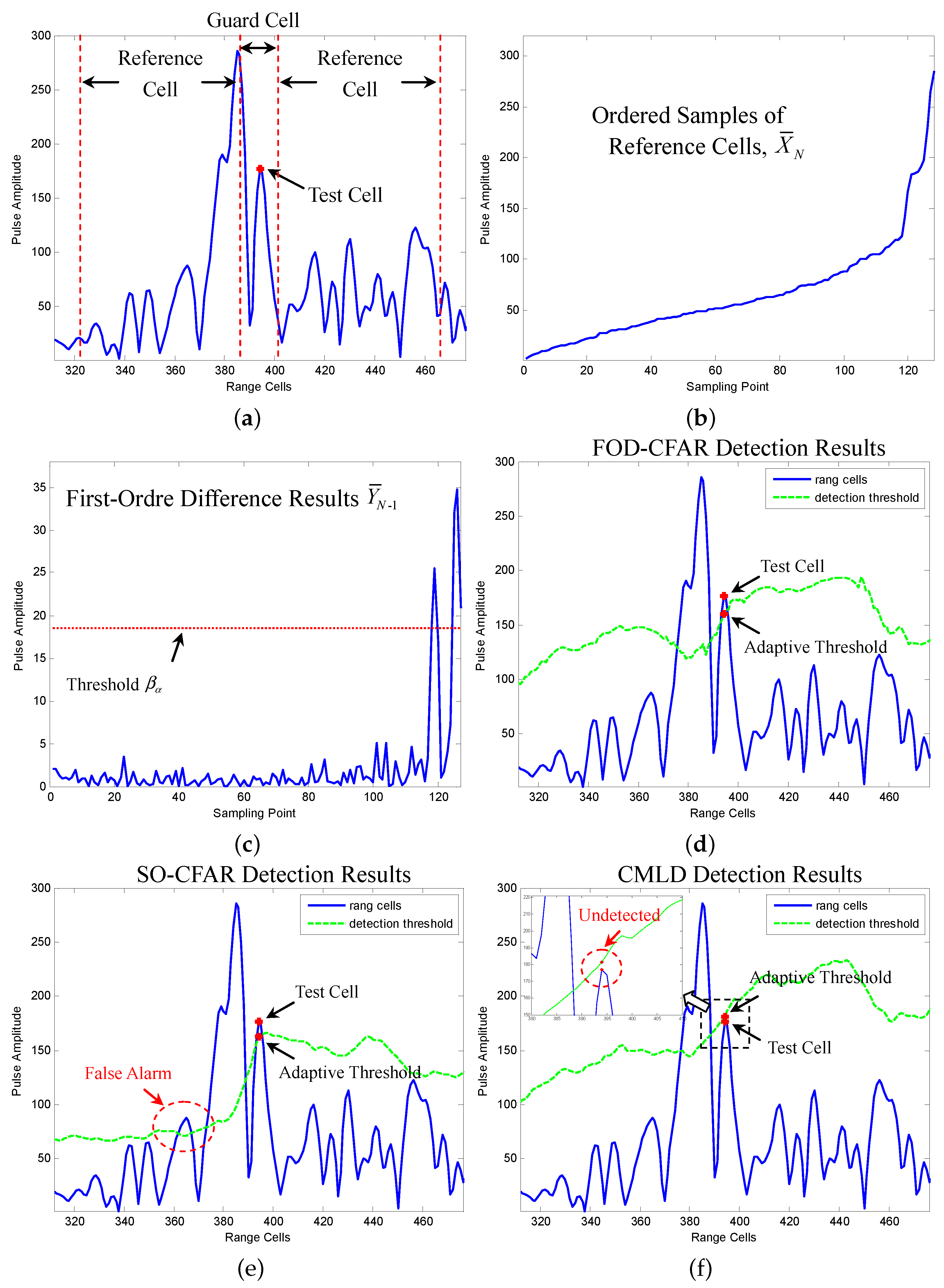
3.1. Idea Behind FOD-CFAR
3.2. Description of the FOD-CFAR Algorithm
- The reference cells are first ranked to form the ordered samples:
- After computing the first-order forward difference of , we obtained:
- We use p lowest cells of ordered samples to calculate the threshold . The implementation method of is described in the next section.
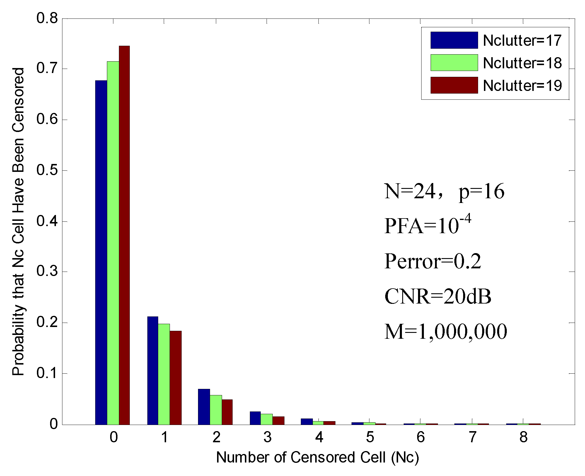
- Then, is compared to the corresponding threshold , and a binary decision is made in favor of or according to the hypothesis test:Hypothesis corresponds to the case where the reference cell is declared nonhomogeneous, while denotes the hypothesis where the reference cell is declared homogeneous. While the hypothesis is true, we find , which is greater than . Then, we decide that the ordered subset corresponds to homogeneous returns. After that, the highest cells will be censored. In the censoring process, k corresponds to the estimated number of samples to be reserved in the reference window, and denotes the estimated number of samples to be censored from the upper end of ordered samples .
- After censoring the unwanted ranked cells, the remaining k samples are combined to form an estimate of the background power level:
- Next, the corresponding scaling factor is selected based on the k and the desired probability of false alarm (PFA). The implementation method of is described in the next section.
- Finally, a target present decision is made if the value of the test cell exceeds the adaptive threshold according to the hypothesis test:Here, denotes the presence of a target in the test cell, while corresponds to the absence of a target in the test cell.
- In the automatic censoring process, the proposed CFAR detector does not require any prior knowledge about the background environment. It makes FOD-CFAR more suitable to a changing environment.
- The detector discussed here employs a fixed detection threshold to reject interference targets, and it is not a cell-by-cell censoring procedure, which allows acceptance or rejection of the ordered cells by performing a successive threshold design. It can bring some benefits to computational efficiency.
4. FOD-CFAR Parameter Selection
4.1. Threshold
4.2. Scaling Factor
5. Performance Results
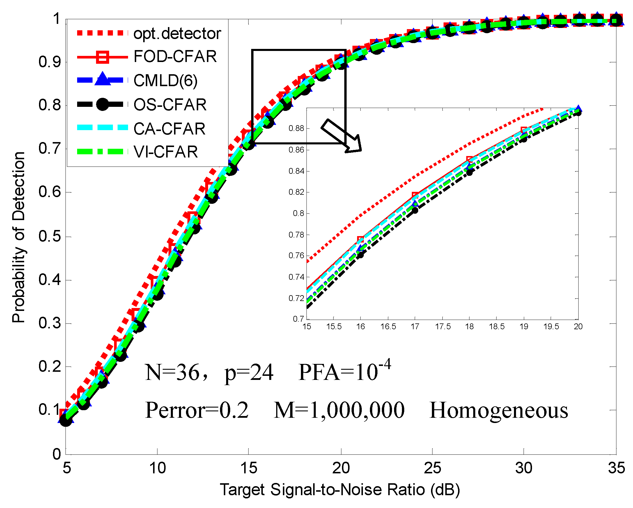
5.1. Scenario 1: Homogeneous Environment
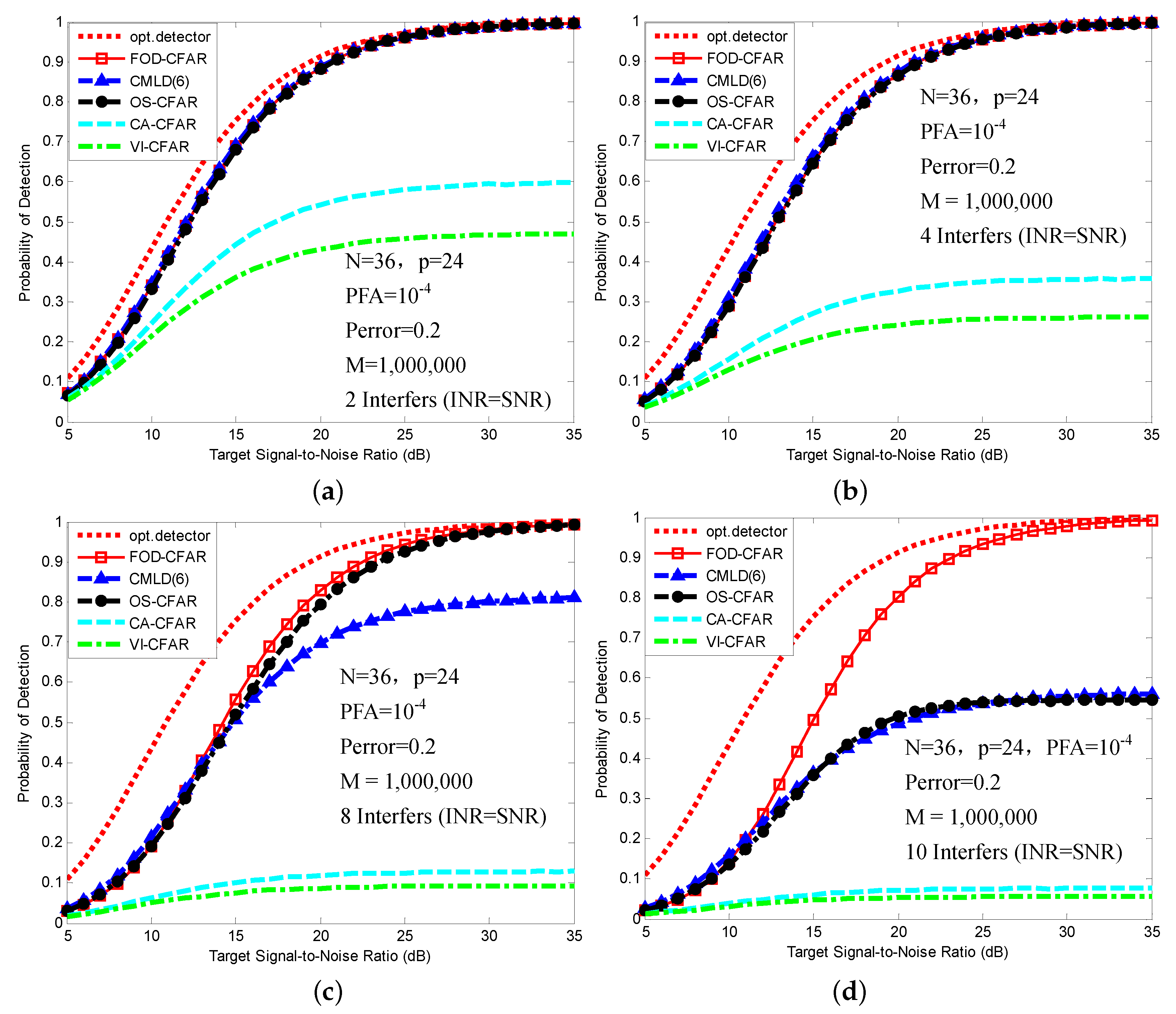
5.2. Scenario 2: Multiple Target Situations
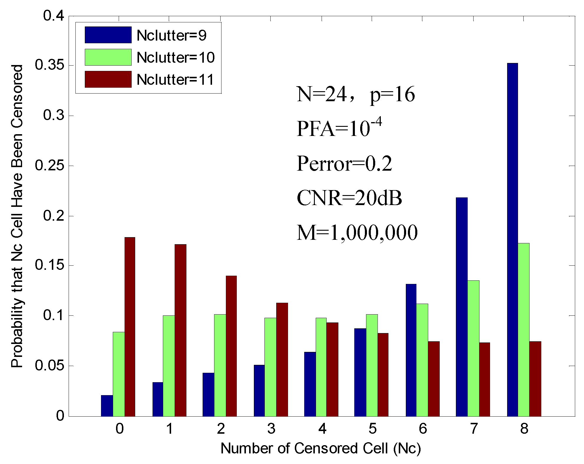
5.3. Scenario 3: Clutter Edge Environment
5.4. Time Complexity Analysis
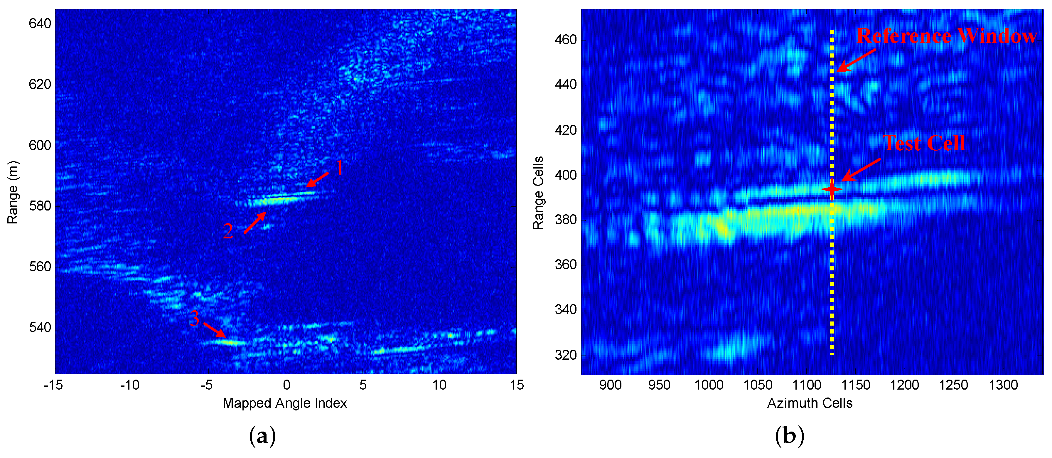
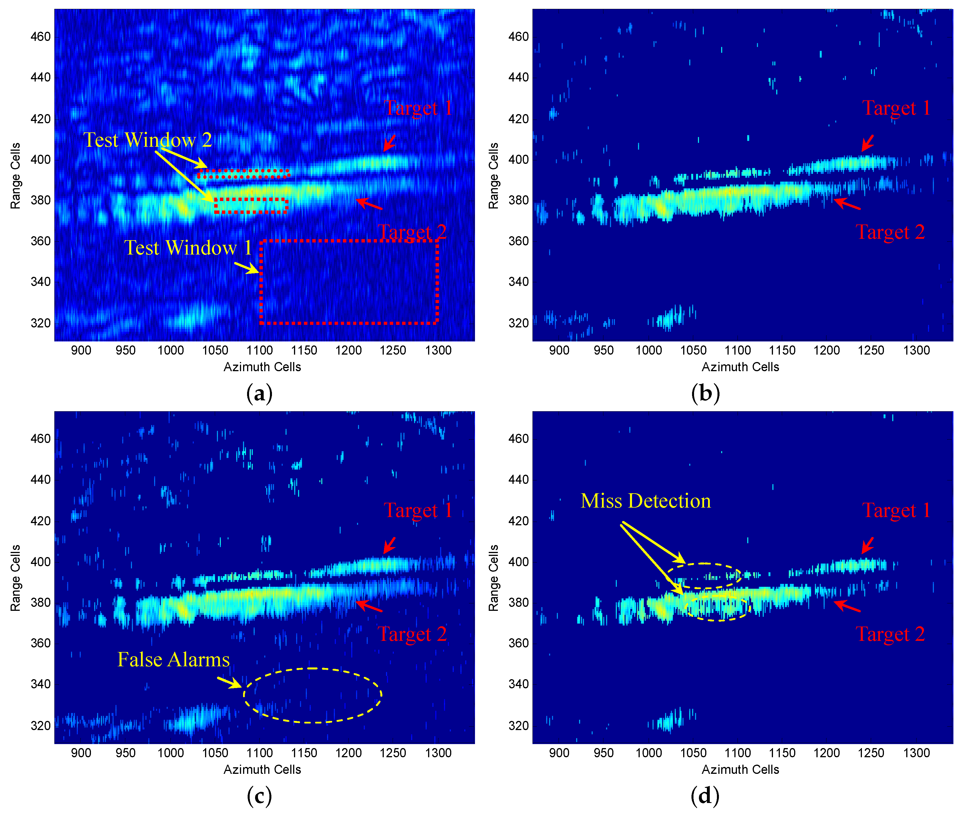
5.5. Experimental Results
6. Conclusions
Acknowledgments
Author Contributions
Conflicts of Interest
References
- Mangogno, A.J. Development of a helicopter obstacle detection and air data. In Proceedings of the IEEE 20th Digital Avionics Conference, Daytona Beach, CA, USA, 14–18 October 2001; pp. 1A41–1A47.
- Almsted, L.D.; Becker, R.C.; Zelenka, R.E. Affordable MMW aircraft collision avoidance system. In Proceedings of the AeroSense’97, International Society for Optics and Photonics, lOrlando, FL, USA, 26 June 1997; pp. 57–63.
- Seidel, C.; Schwartz, I.; Kielhorn, P. Helicopter collision avoidance and brown-out recovery with HELLAS. In Proceedings of the SPIE Europe Security and Defence, International Society for Optics and Photonics, Cardiff, UK, 2 October 2008; pp. 71140G–71140G.
- Bhanu, B.; Das, S.; Roberts, B.; Duncan, D. A system for obstacle detection during rotorcraft low altitude flight. IEEE Trans. Aerosp. Electron. Syst. 1996, 32, 875–897. [Google Scholar] [CrossRef]
- Lynch, D. Introduction to RF Stealth; Scitech Publishing: Raleigh, NC, USA, 2004. [Google Scholar]
- Skolnick, M. Radar Handbook; McGraw-Hill Companies: New York, NY, USA, 2008. [Google Scholar]
- Malaek, S.; Kosari, A. Novel minimum time trajectory planning in terrain following flights. IEEE Trans. Aerosp. Electron. Syst. 2007, 43, 2–12. [Google Scholar] [CrossRef]
- Malaek, S.; Kosari, A. Dynamic based cost functions for TF/TA flights. IEEE Trans. Aerosp. Electron. Syst. 2012, 48, 44–63. [Google Scholar] [CrossRef]
- Ariyur, K.B.; Lommel, P.; Enns, D.F. Reactive inflight obstacle avoidance via radar feedback. In Proceedings of the 2005 IEEE American Control Conference, Portland, OR, USA, 8–10 June 2005; pp. 2978–2982.
- Goshi, D.S.; Case, T.J.; McKitterick, J.B.; Bui, L.Q. Multifunctional millimeter-wave radar system for helicopter safety. In Proceedings of the International Society for Optics and Photonics, SPIE Defense, Security, and Sensing, Baltimore, MD, USA, 23–27 April 2012; pp. 83610A–83610A.
- Kumar, B.A.; Ghose, D. Radar-assisted collision avoidance/guidance strategy for planar flight. IEEE Trans. Aerosp. Electron. Syst. 2001, 37, 77–90. [Google Scholar] [CrossRef]
- Migliaccio, C.; Nguyen, B.; Pichot, C.; Yonemoto, N.; Yamamoto, K.; Yamada, K.; Nasui, H.; Mayer, W.; Gronau, A.; Menzel, W. Millimeter-wave radar for rescue helicopters. In Proceedings of the 9th International Conference on Control, Automation, Robotics and Vision, Singapore, Singapore, 5–8 December 2006; pp. 1–6.
- Yonemoto, N.; Yamamoto, K.; Yamada, K.; Yasui, H.; Tanaka, N.; Migliaccio, C.; Dauvignac, J.Y.; Pichot, C. Performance of obstacle detection and collision warning system for civil helicopters. In Proceedings of the Defense and Security Symposium on International Society for Optics and Photonics, Orlando, FL, USA, 17–21 April 2006; pp. 622608–622608.
- Kwag, Y.K.; Chung, C.H. UAV based collision avoidance radar sensor. In Proceedings of the IEEE International Geoscience and Remote Sensing Symposium, Barcelona, Spain, 23–27 July 2007; pp. 639–642.
- Ma, Q.; Goshi, D.S.; Shih, Y.C.; Sun, M.T. An algorithm for power line detection and warning based on a millimeter-wave radar video. IEEE Trans. Image Process. 2011, 20, 3534–3543. [Google Scholar] [PubMed]
- Goshi, D.; Mai, K.; Liu, Y.; Bui, L. A millimeter-wave sensor development system for small airborne platforms. In Proceedings of the 2012 IEEE Radar Conference (RADAR), Glasgow, UK, 22–25 October 2012; pp. 510–515.
- Finn, H.; Johnson, R. Adaptive detection mode with threshold control as a function of spatially sampled clutter-level estimates. RCA Rev. 1968, 29, 414–464. [Google Scholar]
- Weiss, M. Analysis of some modified cell-averaging CFAR processors in multiple-target situations. IEEE Trans. Aerosp. Electron. Syst. 1982, 18, 102–114. [Google Scholar] [CrossRef]
- Li, Y.; Wei, Y.; Li, B.; Alterovitz, G. Modified Anderson-Darling Test-Based Target Detector in Non-Homogenous Environments. Sensors 2014, 14, 16046–16061. [Google Scholar] [CrossRef] [PubMed]
- Gini, F.; Rangaswamy, M. Knowledge Based Radar Detection, Tracking and Classification; John Wiley & Sons: Hoboken, NJ, USA, 2008. [Google Scholar]
- Smith, M.E.; Varshney, P.K. Intelligent CFAR processor based on data variability. IEEE Trans. Aerosp. Electron. Syst. 2000, 36, 837–847. [Google Scholar] [CrossRef]
- Khalighi, M.A.; Bastani, M.H. Adaptive CFAR processor for nonhomogeneous environments. IEEE Trans. Aerosp. Electron. Syst. 2000, 36, 889–897. [Google Scholar] [CrossRef]
- Sarma, A.; Tufts, D.W. Robust adaptive threshold for control of false alarms. IEEE Signal Process. Lett. 2001, 8, 261–263. [Google Scholar] [CrossRef]
- Tabet, L.; Soltani, F. A generalized switching CFAR processor based on test cell statistics. Signal Image Video Process. 2009, 3, 265–273. [Google Scholar] [CrossRef]
- Kim, J.H.; Bell, M.R. A Computationally Efficient CFAR Algorithm Based on a Goodness-of-Fit Test for Piecewise Homogeneous Environments. IEEE Trans. Aerosp. Electron. Syst. 2013, 49, 1519–1535. [Google Scholar] [CrossRef]
- De Maio, A.; Farina, A.; Foglia, G. Design and experimental validation of knowledge-based constant false alarm rate detectors. IET Radar Sonar Navig. 2007, 1, 308–316. [Google Scholar] [CrossRef]
- Wang, W.; Ji, Y.; Lin, X. A Novel Fusion-Based Ship Detection Method from Pol-SAR Images. Sensors 2015, 15, 25072–25089. [Google Scholar] [CrossRef] [PubMed]
- Hammoudi, Z.; Soltani, F. Distributed CA-CFAR and OS-CFAR detection using fuzzy spaces and fuzzy fusion rules. IEE Radar Sonar Navig. 2004, 151, 135–142. [Google Scholar] [CrossRef]
- Hammoudi, Z.; Soltani, F. Distributed IVI-CFAR detection in non-homogeneous environments. Signal Process. 2004, 84, 1231–1237. [Google Scholar] [CrossRef]
- Cao, T.T. Constant false-alarm rate algorithm based on test cell information. IEE Radar Sonar Navig. 2008, 2, 200–213. [Google Scholar] [CrossRef]
- Trunk, G.V. Range resolution of targets using automatic detectors. IEEE Trans. Aerosp. Electron. Syst. 1978, 14, 750–755. [Google Scholar] [CrossRef]
- Hansen, V.; Sawyers, J. Detectability Loss Due to Greatest of Selection in a Cell-Averaging CFAR. IEEE Trans. Aerosp. Electron. Syst. 1980, 1, 115–118. [Google Scholar] [CrossRef]
- Tan, Y.; Li, Q.; Li, Y.; Tian, J. Aircraft Detection in High-Resolution SAR Images Based on a Gradient Textural Saliency Map. Sensors 2015, 15, 23071–23094. [Google Scholar] [CrossRef] [PubMed]
- Rohling, H. Radar CFAR thresholding in clutter and multiple target situations. IEEE Trans. Aerosp. Electron. Syst. 1983, 19, 608–621. [Google Scholar] [CrossRef]
- Gandhi, P.P.; Kassam, S.A. Analysis of CFAR processors in nonhomogeneous background. IEEE Trans. Aerosp. Electron. Syst. 1988, 24, 427–445. [Google Scholar] [CrossRef]
- Rickard, J.T.; Dillard, G.M. Adaptive detection algorithms for multiple-target situations. IEEE Trans. Aerosp. Electron. Syst. 1977, 13, 338–343. [Google Scholar] [CrossRef]
- Himonas, S.D.; Barkat, M. Automatic censored CFAR detection for nonhomogeneous environments. IEEE Trans. Aerosp. Electron. Syst. 1992, 28, 286–304. [Google Scholar] [CrossRef]
- Farrouki, A.; Barkat, M. Automatic censoring CFAR detector based on ordered data variability for nonhomogeneous environments. IEE Radar Sonar Navig. 2005, 152, 43–51. [Google Scholar] [CrossRef]
- Zaimbashi, A.; Norouzi, Y. Automatic dual censoring cell-averaging CFAR detector in non-homogenous environments. Signal Process. 2008, 88, 2611–2621. [Google Scholar] [CrossRef]
- Boudemagh, N.; Hammoudi, Z. Automatic censoring CFAR detector for heterogeneous environments. AEU-Int. J. Electron. Commun. 2014, 68, 1253–1260. [Google Scholar] [CrossRef]
- Cao, T.T.V.; Palmer, J.; Berry, P.E. False alarm control of CFAR algorithms with experimental bistatic radar data. In Proceedings of the 2010 IEEE Radar Conference, Arlington, USA, 10–14 May 2010; pp. 156–161.
- Wang, C.; Liao, M.; Li, X. Ship detection in SAR image based on the alpha-stable distribution. Sensors 2008, 8, 4948–4960. [Google Scholar] [CrossRef]
- Meng, X. Performance analysis of ordered-statistic greatest of-constant false alarm rate with binary integration for M-sweeps. IEE Radar Sonar Navig. 2010, 4, 37–48. [Google Scholar] [CrossRef]
- Pourmottaghi, A.; Taban, M.; Gazor, S. A CFAR detector in a nonhomogenous Weibull clutter. IEEE Trans. Aerosp. Electron. Syst. 2012, 48, 1747–1758. [Google Scholar] [CrossRef]
- Zaimbashi, A.; Taban, M.R.; Nayebi, M.M.; Norouzi, Y. Weighted order statistic and fuzzy rules CFAR detector for Weibull clutter. Signal Process. 2008, 88, 558–570. [Google Scholar] [CrossRef]
- Cui, G.; Maio, A.; Carotenuto, V.; Pallotta, L. Performance prediction of the incoherent detector for a weibull fluctuating target. IEEE Trans. Aerosp. Electron. Syst. 2014, 50, 2176–2184. [Google Scholar]
- Cui, G.; DeMaio, A.; Piezzo, M. Performance prediction of the incoherent radar detector for correlated generalized Swerling-chi fluctuating targets. IEEE Trans. Aerosp. Electron. Syst. 2013, 49, 356–368. [Google Scholar] [CrossRef]


| () | m | |||||
|---|---|---|---|---|---|---|
| () | 2 | 0.9269 | 0.9757 | 0.9922 | 0.9975 | 0.9998 |
| 4 | 0.8316 | 0.9419 | 0.9811 | 0.9940 | 0.9994 | |
| 8 | 0.4554 | 0.7687 | 0.9187 | 0.9734 | 0.9973 | |
| () | 4 | 0.8490 | 0.9483 | 0.9832 | 0.9947 | 0.9995 |
| 8 | 0.6398 | 0.8646 | 0.9546 | 0.9854 | 0.9985 | |
| 12 | 0.2735 | 0.6454 | 0.8679 | 0.9559 | 0.9955 | |
| () | |||||||
|---|---|---|---|---|---|---|---|
| 0.5 | 0.4 | 0.3 | 0.2 | 0.1 | 0.05 | 0.01 | |
| () | 3.2 | 3.9 | 4.8 | 6.0 | 8.2 | 10.7 | 16.9 |
| () | 3.2 | 3.8 | 4.7 | 5.9 | 8.1 | 10.4 | 16.3 |
| Interference Cell | Censored Cell () | |||
|---|---|---|---|---|
| 15 dB | 20 dB | 25 dB | ||
| 2 | 2 | 61.13% | 75.70% | 81.22% |
| 4 | 4 | 44.73% | 70.02% | 81.49% |
| 8 | 8 | 19.91% | 55.78% | 79.53% |
| 10 | 10 | 11.40% | 46.65% | 76.54% |
| General Parameters | Value |
|---|---|
| Frequency | 35 GHz |
| Flight Speed | 30 m/s |
| Flight Altitude | 200 m |
| Pitch Angle | 20 |
| Scan Coverage | ±15 |
| Horizontal Beam Width | 4 |
| Vertical Beam Width | 4.5 |
| Antenna Scan Rate | 60/s |
| Signal Bandwidth | 200 MHz |
| Pulse width | 1 s |
| PRF | 4000 Hz |
| CFAR Detector | Number of False Alarms (NFA) | Number of Misdetections (NMD) | Response Time (RT) |
|---|---|---|---|
| SO-CFAR | 197 | 154 | 0.81 s |
| CMLD | 0 | 427 | 0.98 s |
| FOD-CFAR | 0 | 246 | 2.44 s |
| Total Number | 8000 | 820 |
© 2016 by the authors; licensee MDPI, Basel, Switzerland. This article is an open access article distributed under the terms and conditions of the Creative Commons Attribution (CC-BY) license (http://creativecommons.org/licenses/by/4.0/).
Share and Cite
Jiang, W.; Huang, Y.; Yang, J. Automatic Censoring CFAR Detector Based on Ordered Data Difference for Low-Flying Helicopter Safety. Sensors 2016, 16, 1055. https://doi.org/10.3390/s16071055
Jiang W, Huang Y, Yang J. Automatic Censoring CFAR Detector Based on Ordered Data Difference for Low-Flying Helicopter Safety. Sensors. 2016; 16(7):1055. https://doi.org/10.3390/s16071055
Chicago/Turabian StyleJiang, Wen, Yulin Huang, and Jianyu Yang. 2016. "Automatic Censoring CFAR Detector Based on Ordered Data Difference for Low-Flying Helicopter Safety" Sensors 16, no. 7: 1055. https://doi.org/10.3390/s16071055
APA StyleJiang, W., Huang, Y., & Yang, J. (2016). Automatic Censoring CFAR Detector Based on Ordered Data Difference for Low-Flying Helicopter Safety. Sensors, 16(7), 1055. https://doi.org/10.3390/s16071055