1. Introduction
Wireless sensor networks (WSNs) are formed by a set of spatially-distributed sensors that connect to each other. Each sensor node is formed by: (i) a micro controller; (ii) one or more sensors; and (iii) a wireless transceiver. These nodes may have some degree of autonomy. Their function is to monitor their physical environment and report to sink nodes, which redirect data to the appropriate destination. A key issue in WSNs is how to deploy the network as efficiently as possible in terms of coverage and energy efficiency. Deployment has a strong impact on connectivity and throughput [
1]. Deployment of large WSNs presents a number of problems [
2]. In many applications, networks have to be deployed over a large, potentially dynamic area, so predefining an optimal configuration may be difficult. Furthermore, if a node breaks or runs out of battery, part of the network might get isolated. WSNs usually rely on a mesh topology, which is more redundant, but also more robust and easier to expand and modify. Unfortunately, it is also hard to set up and maintain.
Deployment can be simplified if WSNs can reconfigure themselves. If a node fails, part of the network may adjust to fill the gap as long as nodes can reposition themselves and/or change its roles. Mobile WSNs (MWSNs) can modify their positions to reorganize the network on a needs basis [
3]. MWSNs are useful both for self-deployment, as nodes can move towards their most adequate position, and self-repair, so live nodes can cover dead ones. In order to move autonomously, MWSNs may be deployed by multiple robots systems (MRSs). In this case, nodes also include motors and sensors, and their micro controllers run a basic control system in addition to the WSN code.
The main goal of MWSN deployment is to use as few nodes as possible to cover a given area and to extend the WSN lifetime as much as possible before batteries need to be replaced. A node battery life mostly depends on the amount of traffic that it is generating/routing, so some parts of the WSN will fail earlier than others. In these cases, robots reorganize their positions to keep it working [
4]. Robot deployment requires autonomous navigation skills, but also coordination and localization techniques. GPS is not appropriate in certain environments due to occlusions and the multi-path effect [
5]. Active localization is typically computationally less expensive than passive localization or tracking, so most MWSN systems rely on received signal strength (RSS)-based triangulation. Sometimes, a static beacon infrastructure is fixed for mobile nodes to locally position themselves [
6,
7]. In these cases, deployed nodes can act themselves as beacons for the rest [
5,
8].
There are two different strategies for autonomous self-deployment [
9,
10]. Deliberative systems build a model of the environment, including the relative locations of the nodes and events, to predict their best deployment positions. This methodology is frequently used for static deployment, where nodes are not expected to move afterwards and distribution needs to be optimized as much as possible [
11]. In MWSNs, a master node gathers information about the whole network, makes all decisions and commands the other nodes where to move. This process is computationally expensive and usually involves techniques like genetic algorithms [
12] or, in order to distribute the calculation, particle swarm optimization [
13,
14,
15] and artificial bee colonies [
16]. In order to reduce the computational complexity, deployment can be incremental, i.e., nodes are deployed one at a time, with each node making use of information gathered by the previously-deployed nodes to determine its ideal deployment location [
5]. Even in this case, deployment requires specific hardware to support intense computation and clearly involves a higher traffic load, especially in the vicinity of the node running the optimization algorithm. Distributed implementations of deliberative algorithms may reduce computational load and provide a better traffic distribution up to some point [
17].
Alternatively, reactive systems consider that local dispersion leads naturally to global dispersion, so each node makes decisions according to local factors, e.g., RSS. This approach involves a lower computational load and less intense, better distributed communication. In exchange, deployment is not necessarily optimized. Reactive systems are distributed by nature.
In this work, we evaluate two different reactive deployment approaches: rule-based deployment and behavior-based deployment. In rule-based deployment algorithms, nodes move following mutually exclusive rules until a termination condition is met: afterward, nodes stay in place [
18,
19]. In behavior-based deployment, each node presents a number of basic nuclear behaviors that are combined into an emergent motion action: a node stops when these behaviors reach an equilibrium, i.e., emergent motion is null. Examples of such algorithms are the well-known virtual potential and forces approaches [
20,
21,
22]. Both rule-based deployment and behavior-based deployment present complementary advantages and drawbacks. Rule-based deployment may be adjusted to conform specific topologies, e.g., bus or ring networks, and to fit environment constraints, e.g., deploy along a land boundary. Furthermore, some nodes usually stop early during deployment, before their odometry-based localization is too affected by errors. Stationary nodes can be used as beacons for RSS-based localization for the rest [
8]. However, these methods tend to return poorer coverage, and deployed networks are hard to recover when nodes start to fail. Furthermore, depending on the resulting topology, the load in the nodes may present significant variations. Behavior-based deployment is usually more popular in MWSNs, and there are many implementations in the field. They typically provide better coverage, and they can rearrange in case a node fails. However, nodes tend to move larger distances on average. Furthermore, localization in these cases is harder because there are no natural beacons: any node may move at any time during deployment depending on the behavior of its surrounding nodes.
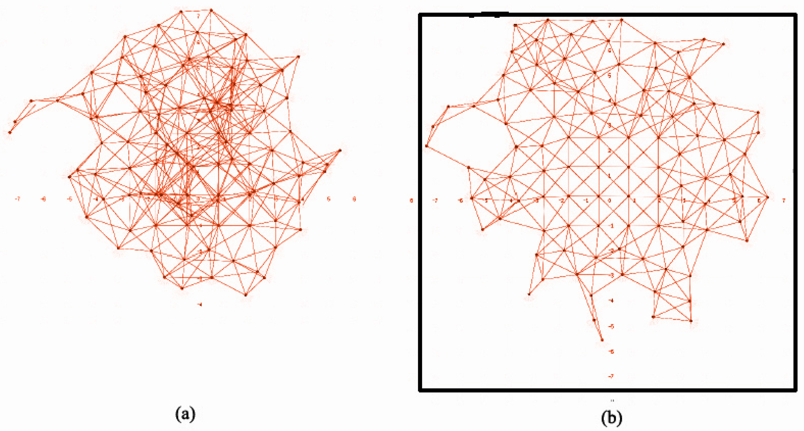
The goal of our work is to compare a representative rule-based deployment algorithm with a behavior-based one. We have specifically chosen the backbone dispersion algorithm (BDA) [
23] and the social potential fields (SPF) [
24] because both are particularly fit to run on a robot swarm. These algorithms are introduced in
Section 2. We have adapted BDA to run on obstacle-avoiding robots during deployment and SPF to preserve connectivity in the network, since it was originally designed for robot swarms. Our evaluation metrics are described in
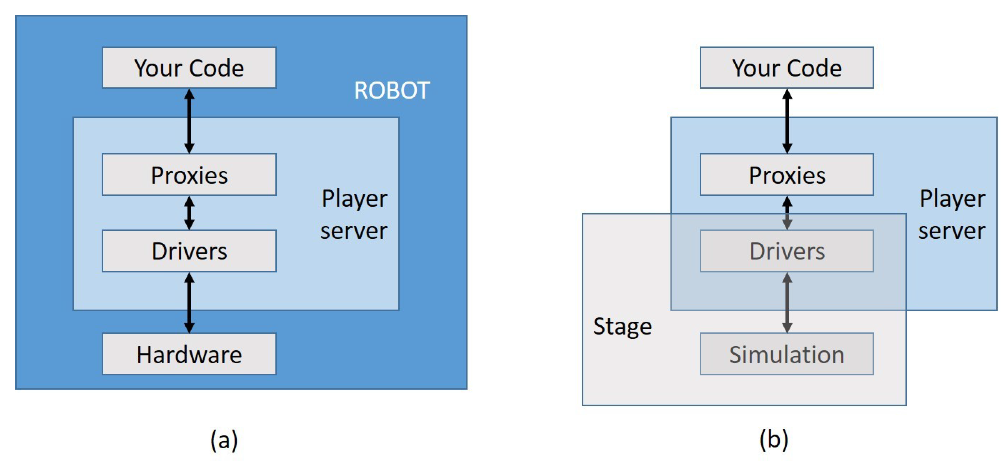
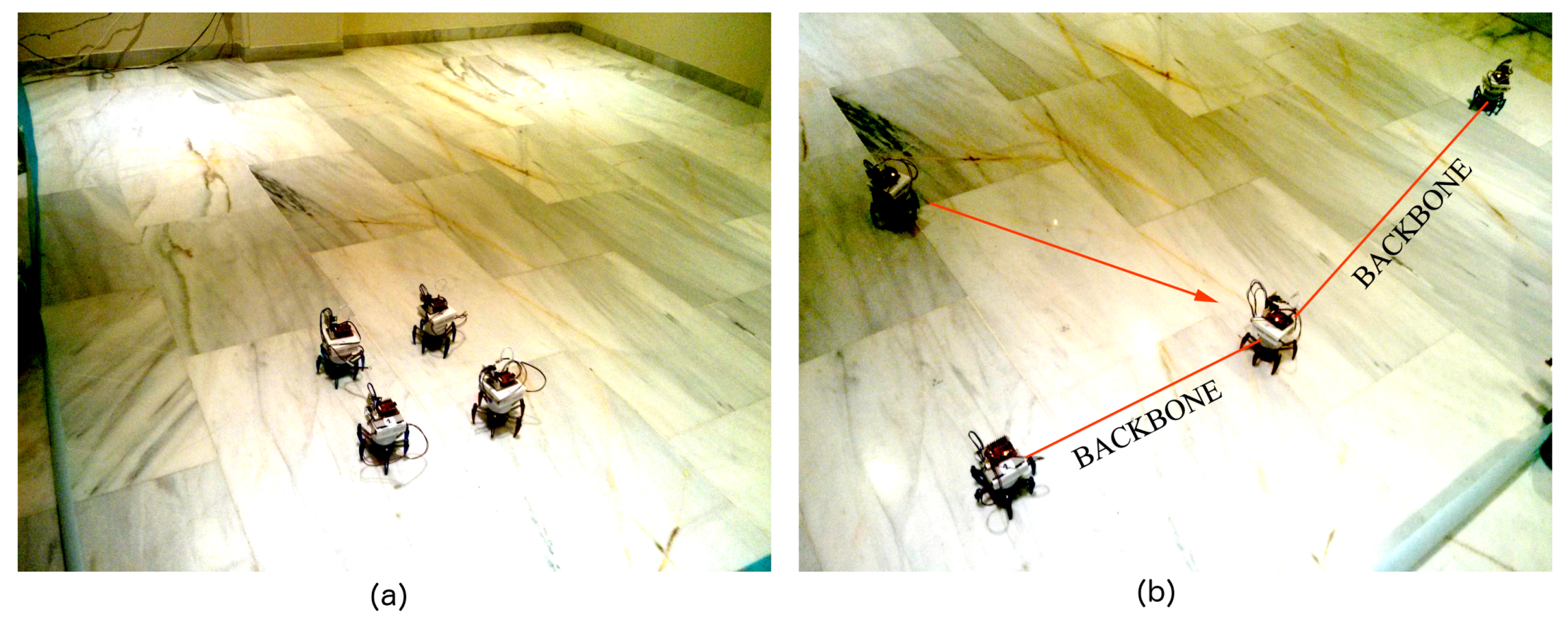
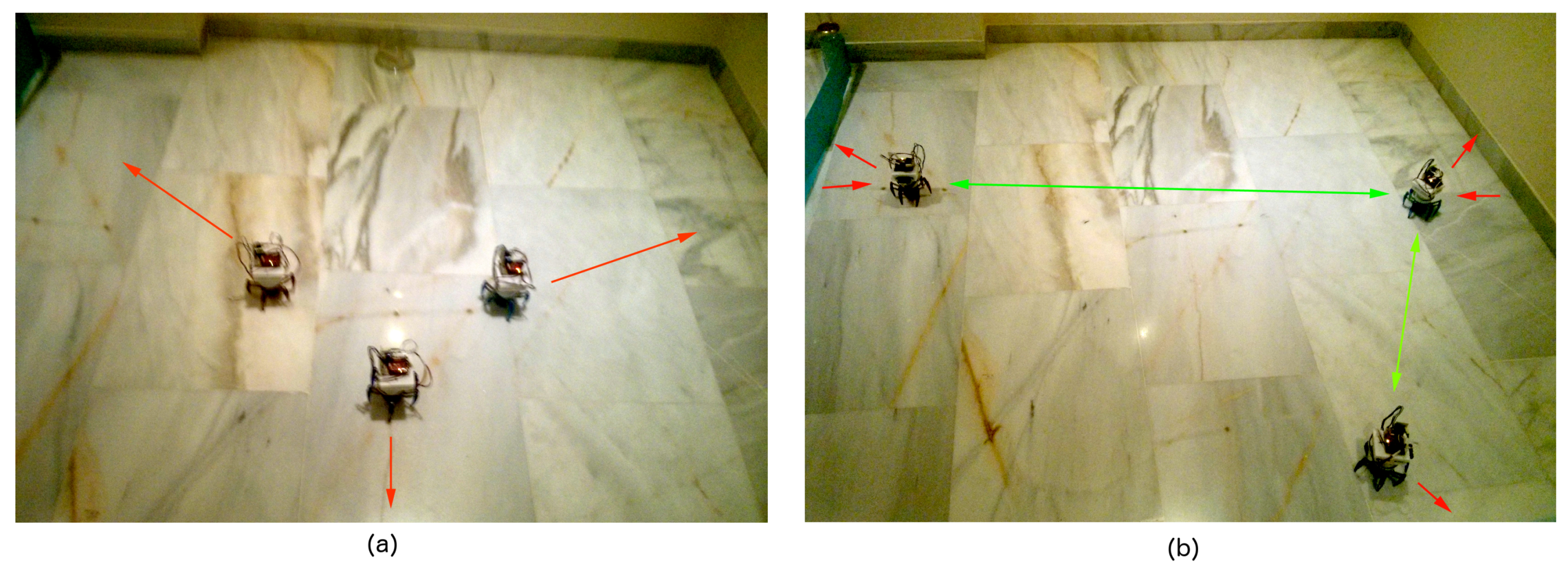
Section 3. Performance depends on the number of nodes in the network. One of the contributions of this work is that we have extended the Player/Stage environment, typically used to test robot behaviors, for network deployment. Hence, we can use the same code in simulations and real tests. Experiments with a large number of nodes have been performed under simulation. We have also validated our conclusions with a very reduced set of nodes in real environments. Networks this small are not fit to extract conclusions about deployment, but these tests confirm the simulation results and provide insight about the difficulties of real-world deployment. Our experimental setup is presented in
Section 4.1. Then, results are presented in
Section 4. Finally, conclusions are presented in
Section 5.
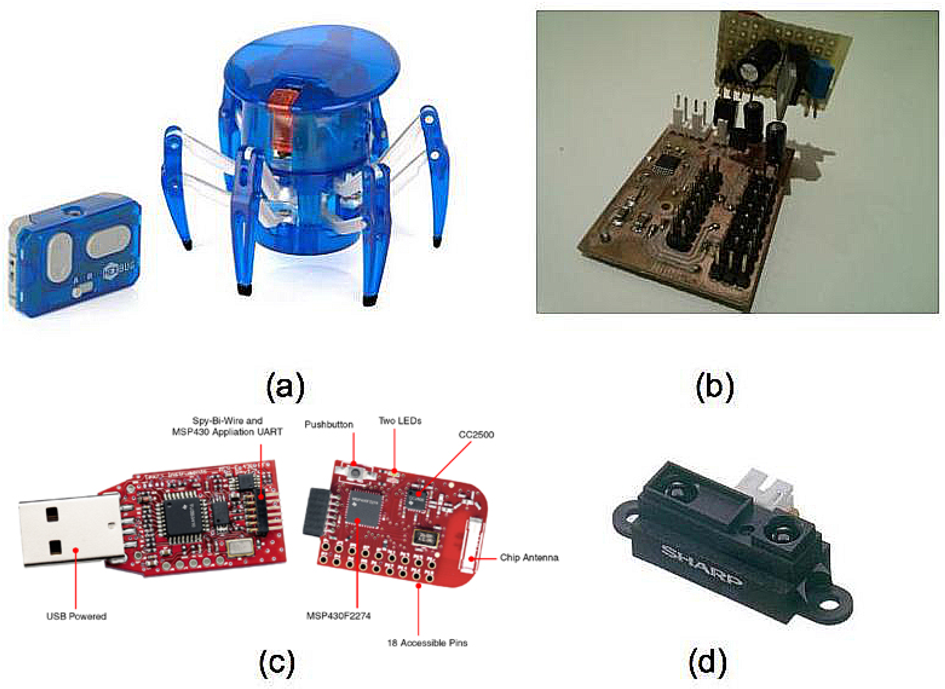
In this work, nodes are robots equipped with a communication module, one or more sensors and a processing unit, plus onboard short-range sensors to prevent collisions.
2. Chosen Deployment Algorithms
The BDA [
23] is a representative rule-based deployment algorithm, where a node moves randomly until it fulfills a termination condition. A node reasons in terms of how many nodes to which it can connect. BDA does not require localization information [
25]. Connectivity is determined by RSS. Collisions between robots are avoided using onboard range sensors. Once a robot stops, it will not move again.
BDA [
23] relies on creating a connected node structure, i.e., a backbone. It uses the following deployment rules. If a node is connected to:
at least two robots and one of them belongs to the backbone: the robot keeps moving randomly and avoiding obstacles to spread the network as much as possible.
a single robot that belongs to the backbone: to prevent loss of connectivity, the robot stops until it gets connected to another robot that travels nearby.
at least a robot, but none of these robots belong to the backbone: the robot joins the backbone, stops and notifies its change of status to the rest of the network.
no robot: the robot moves backwards until it finds some robot with which to connect.
This algorithm is simple and requires little communication among nodes. This implementation is not fit for self-healing because, when nodes stop, they are not supposed to move anymore. Furthermore, it is not adequate for hierarchical networks, where nodes adopt roles depending on their location and connectivity.
We have chosen an implementation of the SPF algorithm to represent behavior-based deployment algorithms. This algorithm was originally proposed for swarm robots [
24], but we have adapted it to mobile WSN deployment. SPF relies on modeling a set of simple attraction and repulsion forces corresponding to goals or constraints, e.g., avoiding collisions, traveling as far as possible from other nodes, etc. We have added an additional behavior for deployment: preserve connectivity with at least another node. All of these forces are combined into an emergent motion vector. Nodes stop moving when this motion vector is null. In practice, nodes stop when this vector is under a threshold
to reduce sensitivity to noise, errors and small changes in the environment. Deployment finishes when all robots stop moving. However, any major change in its input instance (e.g., a nearby node fails or moves) may make a robot move again.
In our implementation of SPF, each robot
i is affected by three types of forces.
Repulsion force(s) that pushes the robot away from nearby robots or obstacles to prevent collisions.
Repulsion force(s) that aims at expanding the network by keeping robots away from each other.
An attraction force (clustering force) . Attraction grows along with to prevent the loss of communication.
is the distance between robots
i and
j. Unlike in BDA, in SPF, we need to estimate robot locations to calculate their relative distances. These locations are always available under simulation. In real rests, locations are estimated using the robots odometry, assuming that they move at a constant speed from their original position, until some of them stop moving. Then, these robots are used as beacons for RSS-based trilateration [
8]. The trilateration method in [
8] would need to be adapted for our specific radiofrequency (RF) chipset for real tests. However, since our number of real robots is so reduced, we simply assume that there will be localization errors. For larger swarms in real tests, it could be advisable to use a transceiver with integrated location, as presented in [
26].
As proposed in [
24], all forces are estimated for every node
j in the vicinity of
i and then combined into an emergent motion vector. Force parameters are heuristically set, depending on the hardware features of the robots, mainly size and RF chipset. In this work, we have heuristically obtained the following parameters from tests with our real robots:
This value has been adjusted so that robots farther than one meter do not affect each other. However, since we have set to 0.5 to avoid oscillations, this force only operates when robots are closer than 60 cm from each other. The same equation applies to robots and static obstacles.
We have adjusted the clustering force parameters to affect robots when they are at least 1.5 m away:
Finally, the second repulsion force is adjusted to keep a distance of approximately two meters between each of two robots:
We use these parameters obtained from real robots also in simulations. The overall behavior of the network is that nodes tend to move away from each other in every direction, avoiding collisions with each other and any obstacle in the way and preserving connectivity to cover an area as large as they can. No specific structure is constructed in this case.
3. Evaluation Parameters
Evaluation of network deployment requires the definition of a set of quality parameters.
Coverage is a typical quality measure in networks. Gage [
27] defines three types of coverage: (i) blanket coverage, focused on achieving a static arrangement of nodes that maximizes the total detection area; (ii) barrier coverage, focused on minimizing the probability of undetected penetration through the barrier; and (iii) sweep coverage, equivalent to a moving barrier. The most fitting one for our work is blanket coverage, i.e., any point of the region is sensed by at least one sensor. If a single node
i covers a round area
, given
N sensors in a full area
A, coverage
C can be calculated as the ratio between the union ∪ of all
and
A:
Equation (
4) can be modeled using a probabilistic grid of
M cells [
28], where we assign to each cell
i a probability
of detecting an event on that specific cell. Several nodes might detect an event at cell
i independently, so we obtain
in terms of the probability of an event going undetected at cell
i (
):
N being the number of nodes and
being the probability of node
j detecting an event at cell
i.
Then, coverage
C is obtained as:
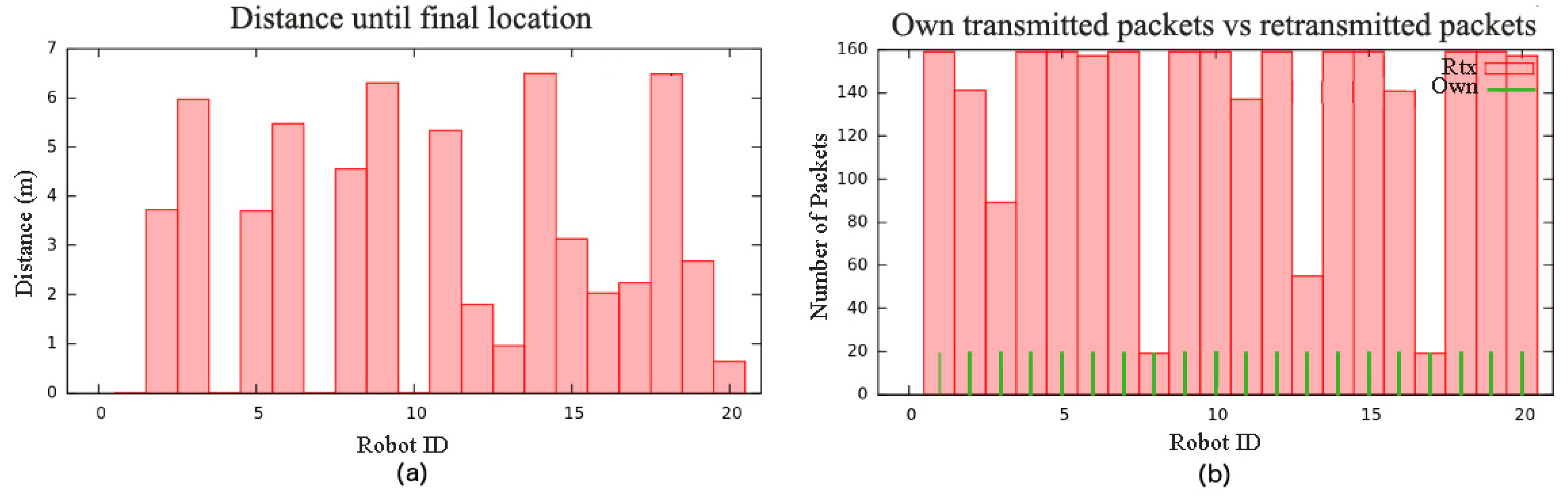
Energetic efficiency is another accepted quality parameter in mesh networks. There are two different energy costs in these networks: (i) deployment and (ii) maintenance. Deployment costs mostly depend on two parameters [
29]: distance
d traveled by each node to its final location; and time
t to reach its final location. After deployment is complete, energy cost is usually related to how homogeneously nodes are distributed. Uniformity
U for
N nodes can be defined as:
being the number of nodes in the vicinity of node
i,
being the distance between nodes
i and
j and
being the average distance between node
i and its closest nodes. A high
U usually leads to higher network lifetime because traffic load tends to be better distributed among nodes.
The network lifetime also depends on energy consumption.
Energy consumption depends on many factors, including separation among nodes, routing strategies and packet losses. In order to evaluate them indirectly, energetic efficiency can be roughly approximated by the average power that nodes require to send a message to the network
:
being the average power required at node
i to send a message to the rest of the network, obtained as:
being the power required to send a message from node
i to node
j.
In networks where messages need to be retransmitted through
k nodes, it is necessary to add the power required for each hop:
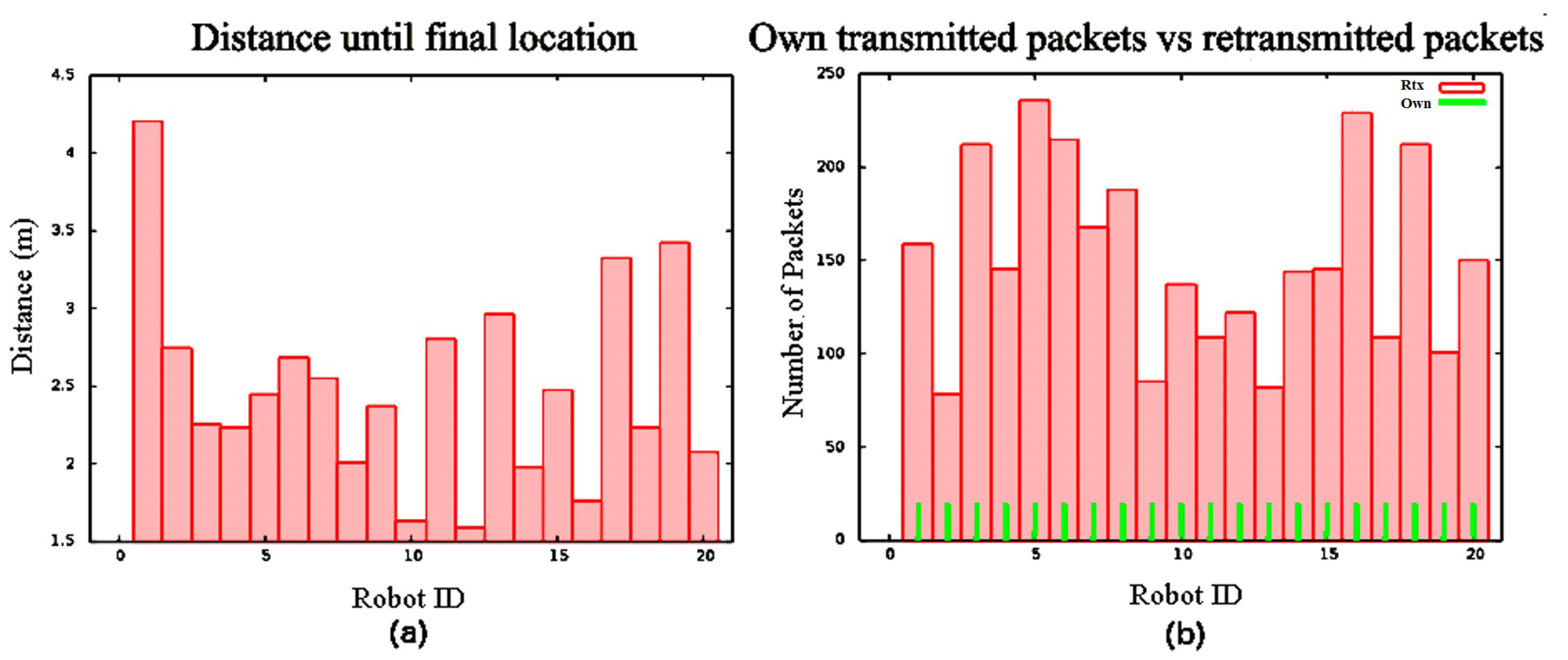
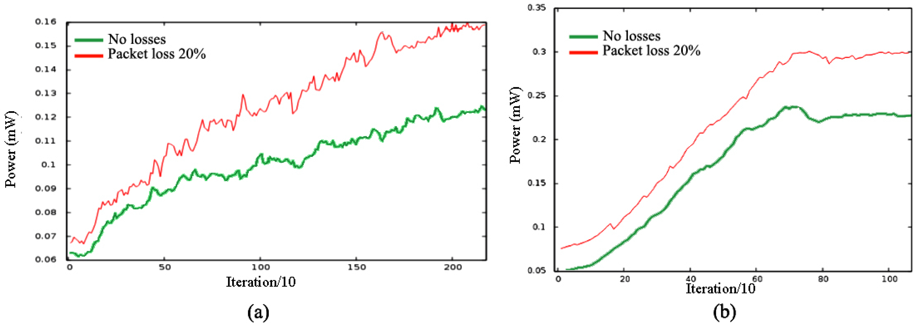
In this work, we are also going to measure unbalance in the network after deployment as the ratio between the number of messages that the most loaded node is routing with respect to the number of messages transmitted by the least loaded node. When mesh networks are not well balanced, some nodes run out of battery much earlier than others and full areas of the network may get disconnected. Unbalance is also related to the deviation in the number of routed packages per sent message in the network (). A large deviation means that some nodes are routing far more messages than others.
5. Conclusions
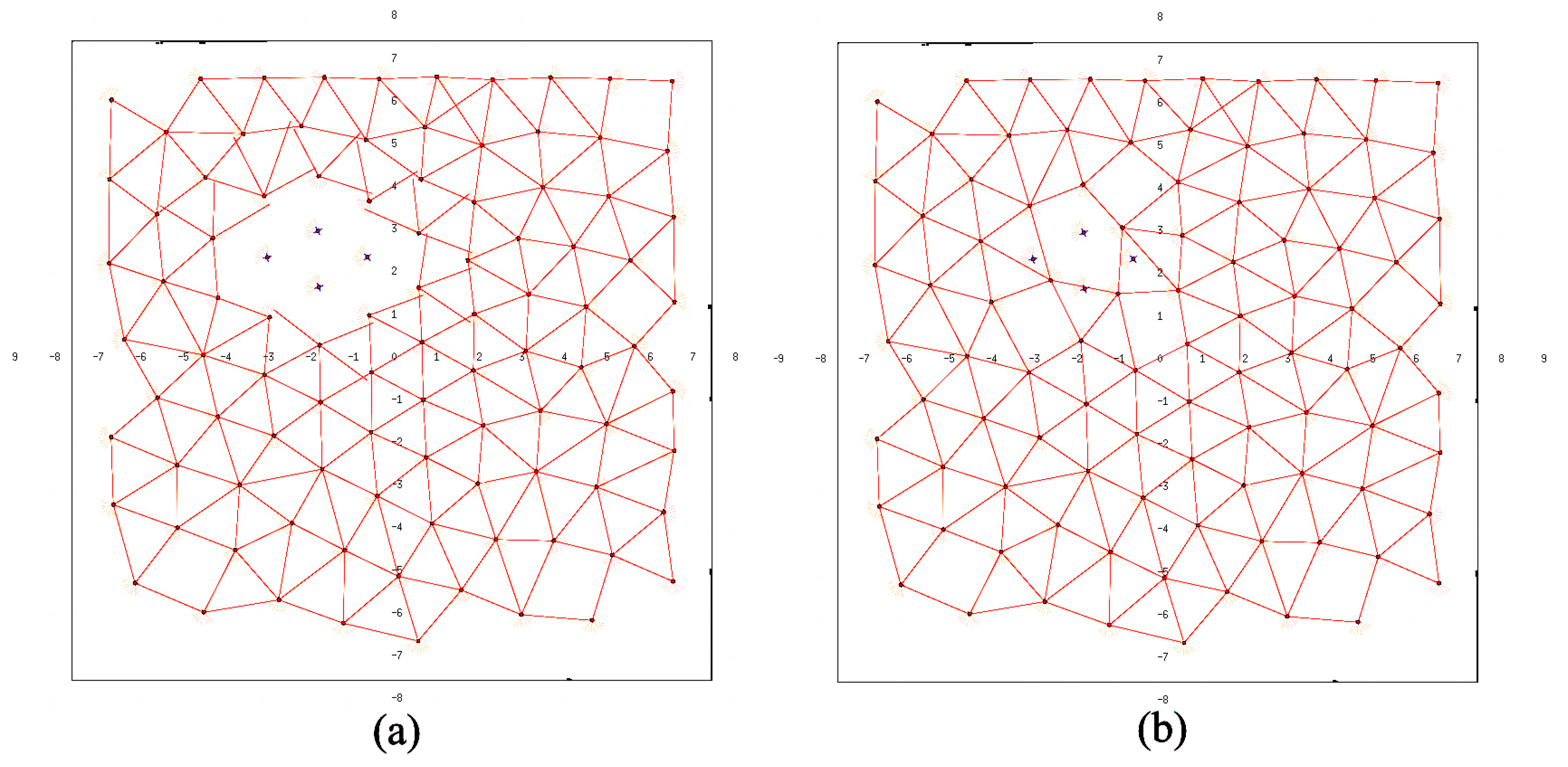
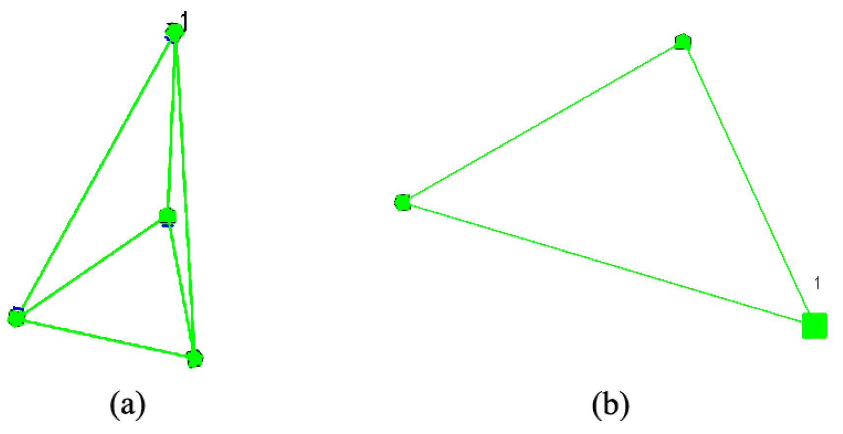
This work has presented an experimental evaluation of rule-based (BDA) and behavior-based (SPF) reactive deployment algorithms for mobile WSNs. Both algorithms have been extensively tested under simulation in environments with and without obstacles for different numbers of nodes. Conclusions extracted from simulations have been validated in a real environment using a very reduced number of nodes. These tests also provided insight about the effect of noise and errors in the evaluated parameters. However, results in real environments cannot be conclusive unless a much larger number of nodes is involved in the tests.
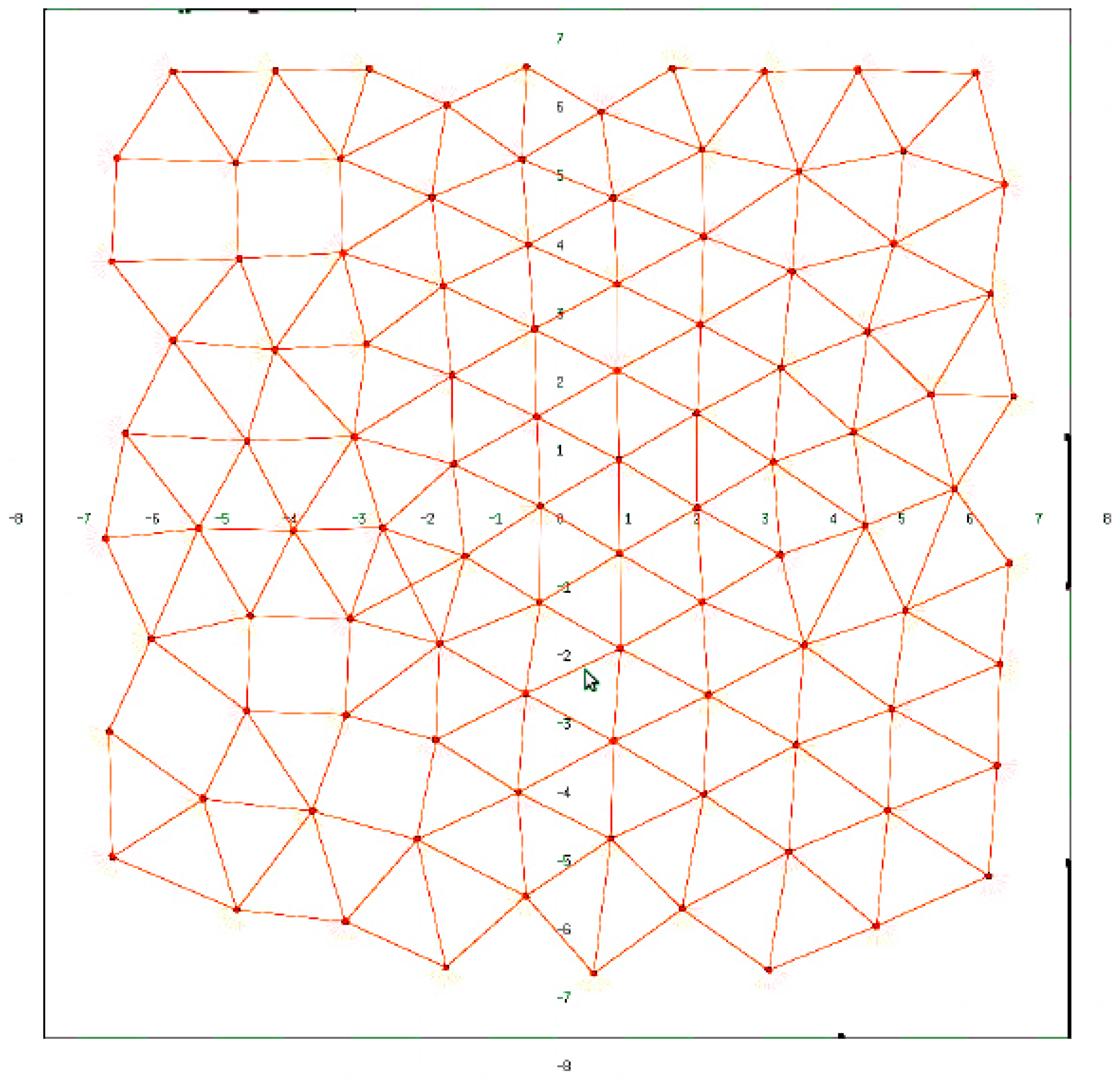
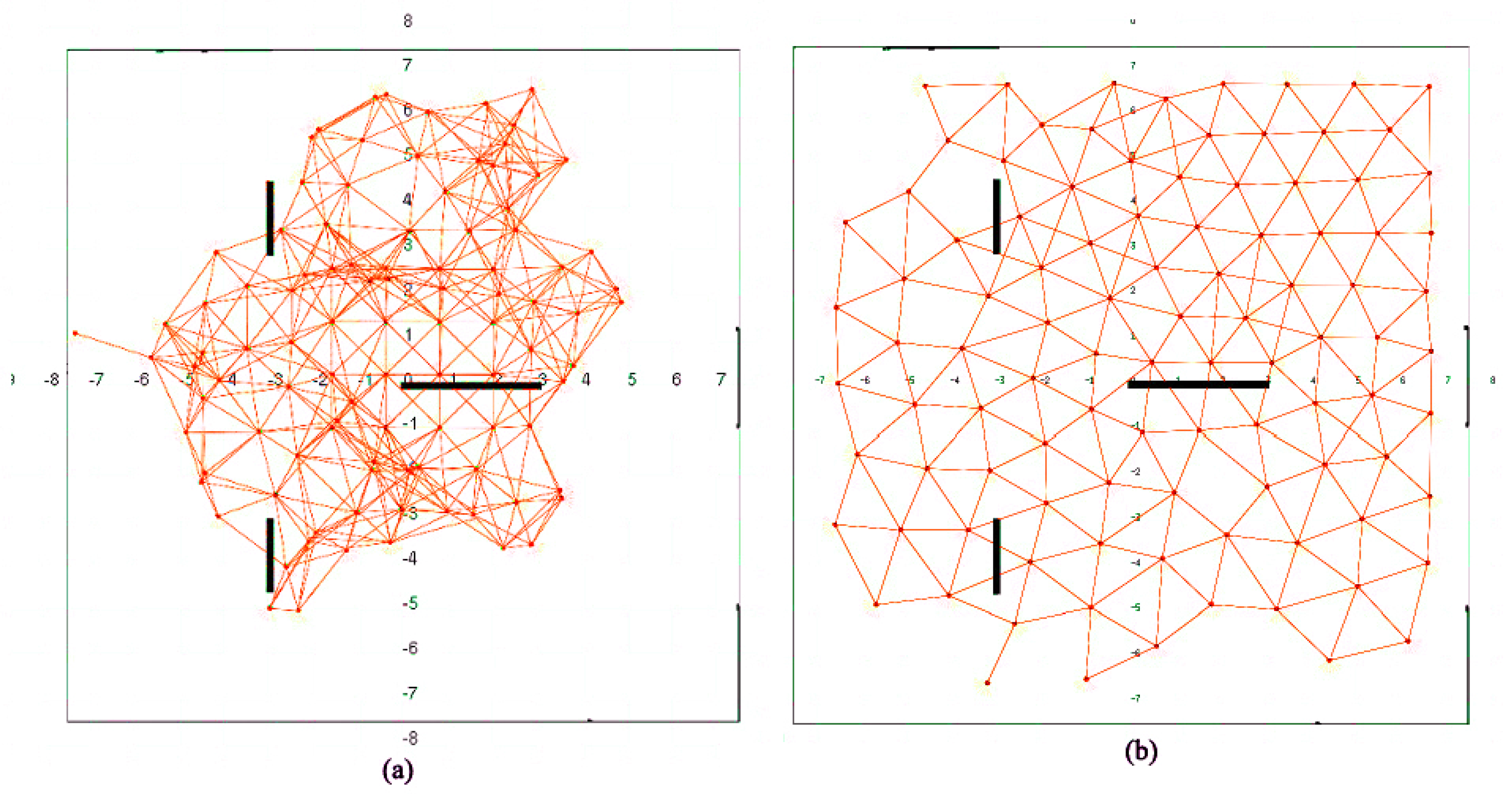
The main conclusions of our evaluations are the following ones. SPF provides faster and more uniform deployment and a better coverage. Furthermore, the network load is better balanced after deployment in this case, meaning that although some nodes transmit more messages than others, unbalance is not as large as after BDA deployment. A better balance leads to a longer network life. Average power and after deployment are actually greater in SPF, mostly because nodes are more separated. However, these parameters may change from one node to the next, contributing to unbalance. SPF deployment also adapts better than BDA to areas with obstacles. All of these effects become more significant in large networks. BDA, however, is less dependent on localization and may offer better results if deployment needs to follow a set of fixed rules.
In brief, SPF seems more suitable for deployment in large, dynamic, unstructured areas, as long as node localization is reliable. Future work will focus on extending this study to hierarchical WSNs.


 ,
, 


