
Joint Maximum Likelihood Time Delay Estimation of Unknown Event-Related Potential Signals for EEG Sensor Signal Quality Enhancement


 and
and 
Abstract
:1. Introduction
2. Signal Model and Conventional TDE Schemes
3. Proposed Optimum and Sub-Optimum TDE Scheme
3.1. Proposed Optimum TDE Scheme
3.2. Proposed Sub-Optimum TDE Scheme
4. Performance Evaluation
4.1. Simulation Setup
4.1.1. Signal Selection
4.1.2. TDE Performance Evaluation
4.2. Simulation Result
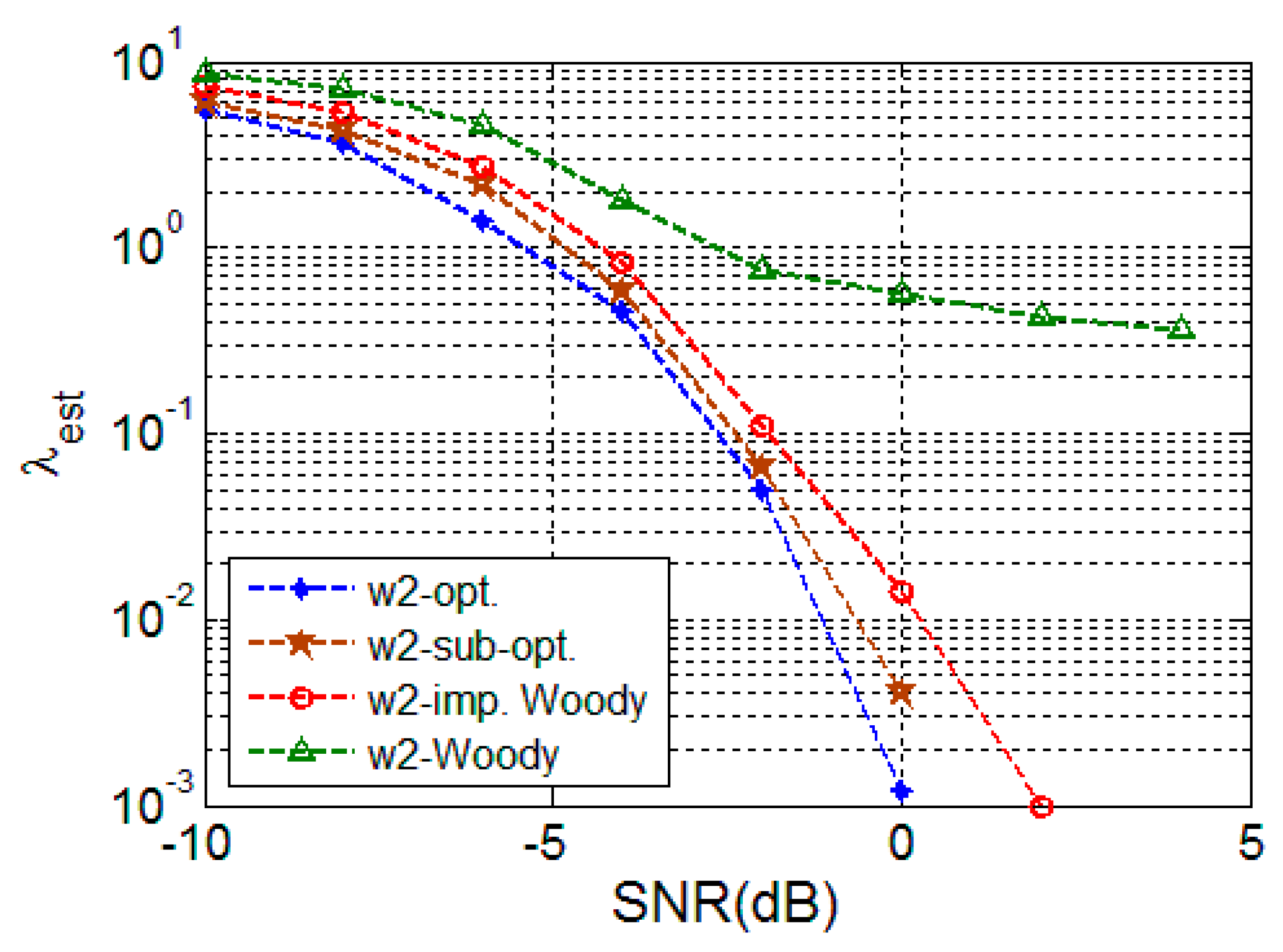
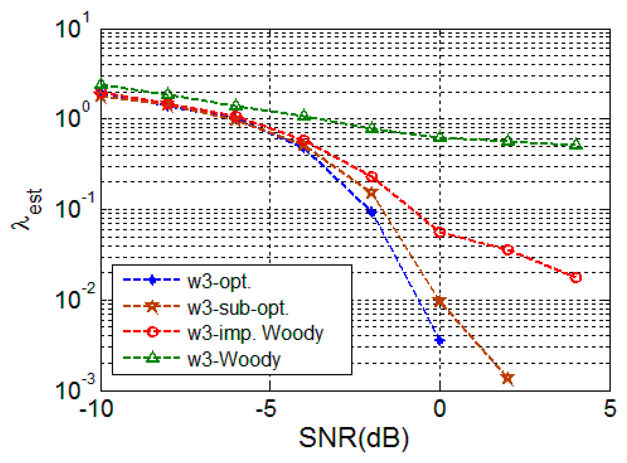
4.2.1. Random Signal
4.2.2. Deterministic Signal
4.2.3. EEG Signal
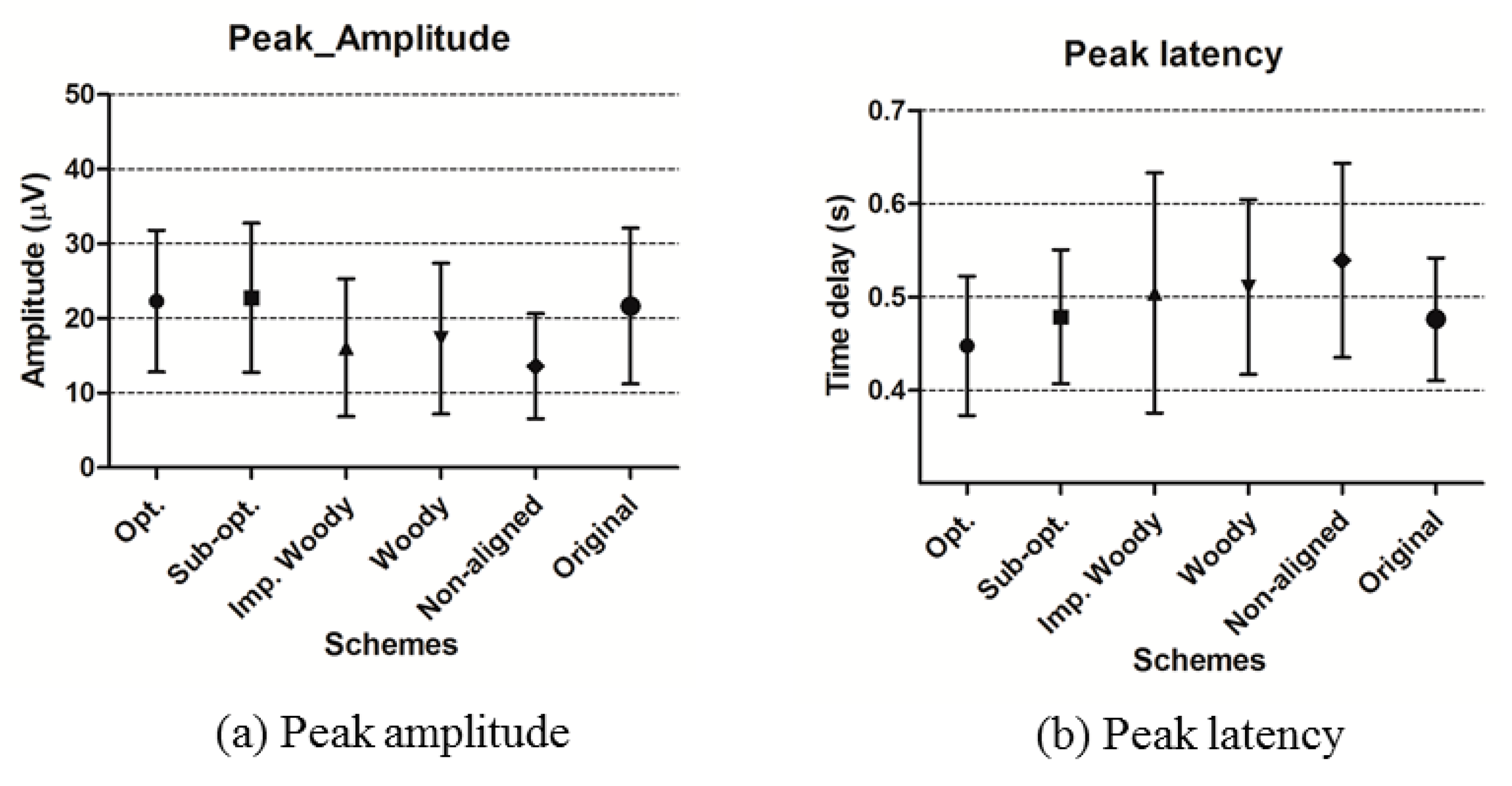
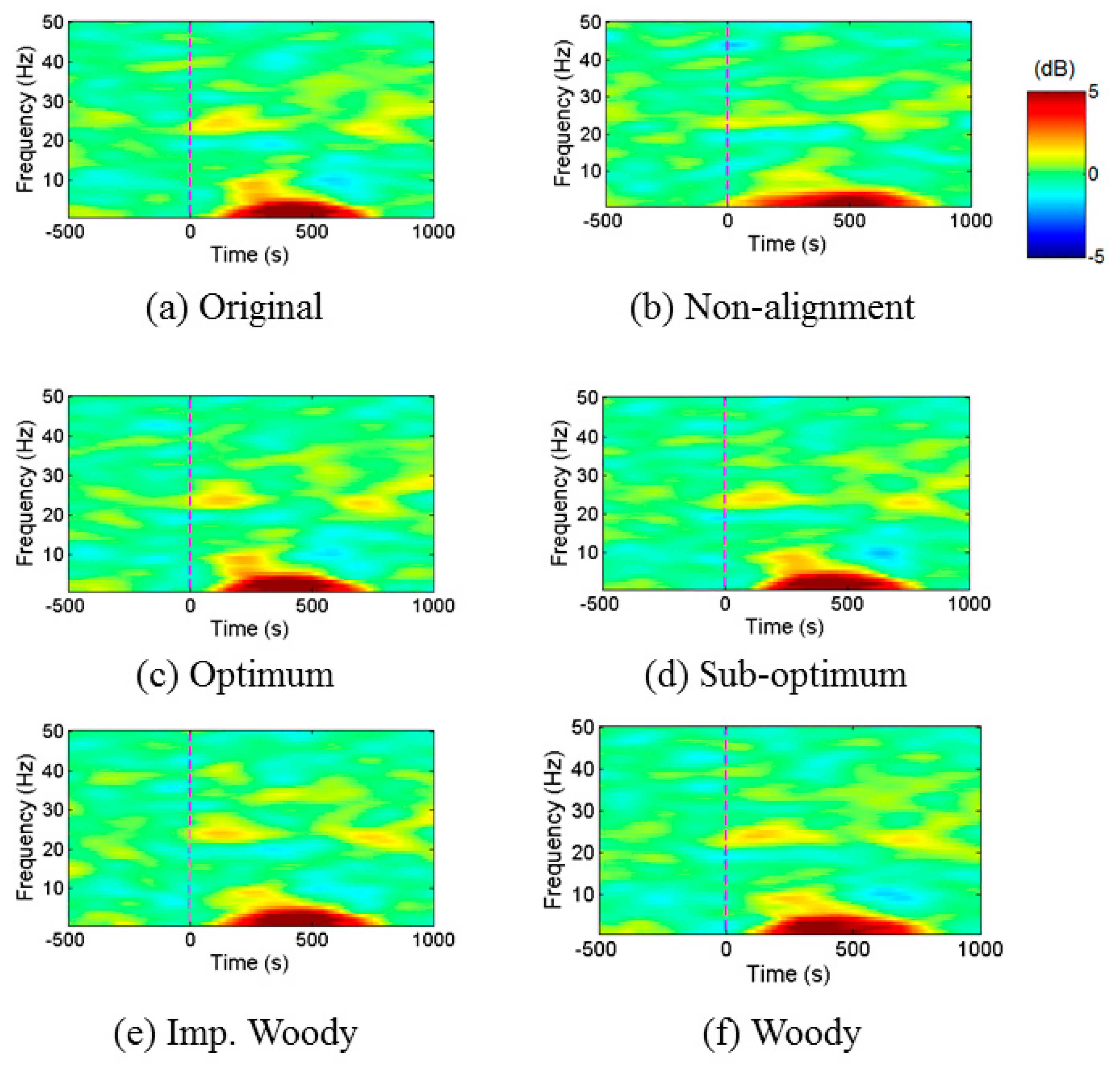
4.2.4. ERP Analysis
5. Conclusions
Acknowledgments
Author Contributions
Conflicts of Interest
References
- Liao, L.-D.; Wang, I.-J.; Chen, S.-F.; Chang, J.-Y.; Lin, C.-T. Design, fabrication and experimental validation of a novel dry-contact sensor for measuring electroencephalography signals without skin preparation. Sensors 2011, 11, 5819–5834. [Google Scholar] [CrossRef] [PubMed]
- Lopez-Gordo, M.A.; Sanchez-Morillo, D.; Pelayo Valle, F. Dry EEG electrodes. Sensors 2014, 14, 12847–12870. [Google Scholar] [CrossRef] [PubMed]
- Alba, N.A.; Sclabassi, R.J.; Sun, M.; Cui, X.T. Novel hydrogel-based preparation-free EEG electrode. IEEE Trans. Neural Syst. Rehabil. Eng. 2010, 18, 415–423. [Google Scholar] [CrossRef] [PubMed]
- Lu, J.; Xie, K.; McFarland, D.J. Adaptive spatio-temporal filtering for movement related potentials in EEG-based brain-computer interfaces. IEEE Trans. Neural Syst. Rehabil. Eng. 2014, 22, 847–857. [Google Scholar] [PubMed]
- Spyrou, L.; Sanei, S.; Took, C.C. Estimation and location tracking of the P300 subcomponents from single-trial EEG. In Proceedings of the IEEE International Conference on Acoustics, Speech and Signal Processing, Honolulu, HI, USA, 16–20 April 2007; pp. 1149–1152.
- Speier, W.; Arnold, C.; Lu, J.; Deshpande, A.; Pouratian, N. Integrating language information with a hidden Markov model to improve communication rate in the P300 speller. IEEE Trans. Neural Syst. Rehabil. Eng. 2014, 22, 678–684. [Google Scholar] [CrossRef] [PubMed]
- Friedman, D. Cognition and aging: A highly selective overview of event-related potential (ERP) data. J. Clin. Exp. Neuropsychol. 2003, 25, 702–720. [Google Scholar] [CrossRef] [PubMed]
- Thornton, A.R.D.; Harmer, M.; Lavoie, B.A. Selective attention increases the temporal precision of the auditory N-100 event-related potential. Hear. Res. 2007, 230, 73–79. [Google Scholar] [CrossRef] [PubMed]
- McFarland, D.J.; Cacace, A.T. Separating stimulus-locked and unlocked components of the auditory event-related potential. Hear. Res. 2004, 193, 111–120. [Google Scholar] [CrossRef] [PubMed]
- Daou, H.; Labeau, F. Dynamic dictionary for combined EEG compression and seizure detection. IEEE J. Biomed. Health Inf. 2014, 18, 247–256. [Google Scholar] [CrossRef] [PubMed]
- Gath, I.; Feuerstein, C.; Pham, D.T.; Rondouin, G. On the tracking of rapid dynamic changes in seizure EEG. IEEE Trans. Biomed. Eng. 1992, 39, 952–958. [Google Scholar] [CrossRef] [PubMed]
- Harris, B.; Gath, I.; Rondouin, G.; Feuerstein, C. On time delay estimation of epileptic EEG. IEEE Trans. Biomed. Eng. 1994, 41, 820–829. [Google Scholar] [CrossRef] [PubMed]
- Meste, O.; Rix, H. Jitter statistics estimation in alignment processes. Signal Process. 1996, 51, 41–53. [Google Scholar] [CrossRef]
- Aricò, P.; Aloise, F.; Schettini, F.; Salinari, S.; Mattia, D.; Cincotti, F. Influence of P300 latency jitter on event related potential-based brain–computer interface performance. J. Neural Eng. 2014, 11, 035008. [Google Scholar] [CrossRef] [PubMed]
- Franz, M.; Nickel, M.; Ritter, A.; Miltner, W.; Weiss, T. Somatosensory spatial attention modulates amplitudes, latencies, and latency JITTER of laser-evoked brain potentials. J. Neurophysiol. 2015, 113, 2760–2768. [Google Scholar] [CrossRef] [PubMed]
- Lainscsek, C.; Hernandez, M.E.; Poizner, H.; Sejnowski, T.J. Delay differential analysis of electroencephalographic data. Neural Comput. 2015, 27, 615–627. [Google Scholar] [CrossRef] [PubMed]
- Chen, J.; Benesty, J.; Huang, Y. Robust time delay estimation exploiting redundancy among multiple microphones. IEEE Trans. Speech Audio Process. 2003, 11, 549–557. [Google Scholar] [CrossRef]
- Wen, F.; Wan, Q. Robust time delay estimation for speech signals using information theory: A comparison study. EURASIP J. Audio Speech Music Process. 2011, 2011, 1–10. [Google Scholar] [CrossRef]
- Woody, C.D. Characterization of an adaptive filter for the analysis of variable latency neuroelectric signals. Med. Biol. Eng. 1967, 5, 539–554. [Google Scholar] [CrossRef]
- Tuan, P.D.; Möcks, J.; Köhler, W.; Gasser, T. Variable latencies of noisy signals: Estimation and testing in brain potential data. Biometrika 1987, 74, 525–533. [Google Scholar] [CrossRef]
- Li, R.; Principe, J.C.; Bradley, M.; Ferrari, V. A spatiotemporal filtering methodology for single-trial ERP component estimation. IEEE Trans. Biomed. Eng. 2009, 56, 83–92. [Google Scholar] [PubMed]
- Jarchi, D.; Sanei, S.; Principe, J.C.; Makkiabadi, B. A new spatiotemporal filtering method for single-trial estimation of correlated ERP subcomponents. IEEE Trans. Biomed. Eng. 2011, 58, 132–143. [Google Scholar] [CrossRef] [PubMed]
- Cabasson, A.; Meste, O. Time delay estimation: A new insight into the Woody’s method. IEEE Signal Process. Lett. 2008, 15, 573–576. [Google Scholar] [CrossRef]
- Graichen, U.; Witte, H.; Haueisen, J. Analysis of induced components in electroencephalograms using a multiple correlation method. BioMed. Eng. Online 2009, 8. [Google Scholar] [CrossRef] [PubMed]
- Jaśkowski, P. Amplitudes and latencies of single-trial ERP’s estimated by a maximum-likelihood method. IEEE Trans. Biomed. Eng. 1999, 46, 987–993. [Google Scholar] [CrossRef] [PubMed]
- Mäkinen, V.; Tiitinen, H.; May, P. Auditory event-related responses are generated independently of ongoing brain activity. Neuroimage 2005, 24, 961–968. [Google Scholar] [CrossRef] [PubMed]
- Makeig, S.; Delorme, A.; Westerfield, M.; Jung, T.-P.; Townsend, J.; Courchesne, E.; Sejnowski, T.J. Electroencephalographic brain dynamics following manually responded visual targets. PLoS Biol. 2004, 2, 747–762. [Google Scholar] [CrossRef] [PubMed]
- Gasser, T.; Möcks, J.; Verleger, R. SELAVCO: A method to deal with trial-to-trial variability of evoked potentials. Electroencephal. Clin. Neurophysiol. 1983, 55, 717–723. [Google Scholar] [CrossRef]
- Möcks, J.; Gasser, T.; Tuan, P.D. Variability of single visual evoked potentials evaluated by two new statistical tests. Electroencephal. Clin. Neurophysiol. 1984, 57, 571–580. [Google Scholar] [CrossRef]
- Delorme, A.; Makeig, S. EEGLAB: An open source toolbox for analysis of single-trial EEG dynamics including independent component analysis. J. Neurosci. Methods 2004, 134, 9–21. [Google Scholar] [CrossRef] [PubMed]


© 2016 by the authors; licensee MDPI, Basel, Switzerland. This article is an open access article distributed under the terms and conditions of the Creative Commons Attribution (CC-BY) license (http://creativecommons.org/licenses/by/4.0/).
Share and Cite
Kim, K.; Lim, S.-H.; Lee, J.; Kang, W.-S.; Moon, C.; Choi, J.-W. Joint Maximum Likelihood Time Delay Estimation of Unknown Event-Related Potential Signals for EEG Sensor Signal Quality Enhancement. Sensors 2016, 16, 891. https://doi.org/10.3390/s16060891
Kim K, Lim S-H, Lee J, Kang W-S, Moon C, Choi J-W. Joint Maximum Likelihood Time Delay Estimation of Unknown Event-Related Potential Signals for EEG Sensor Signal Quality Enhancement. Sensors. 2016; 16(6):891. https://doi.org/10.3390/s16060891
Chicago/Turabian StyleKim, Kyungsoo, Sung-Ho Lim, Jaeseok Lee, Won-Seok Kang, Cheil Moon, and Ji-Woong Choi. 2016. "Joint Maximum Likelihood Time Delay Estimation of Unknown Event-Related Potential Signals for EEG Sensor Signal Quality Enhancement" Sensors 16, no. 6: 891. https://doi.org/10.3390/s16060891
APA StyleKim, K., Lim, S.-H., Lee, J., Kang, W.-S., Moon, C., & Choi, J.-W. (2016). Joint Maximum Likelihood Time Delay Estimation of Unknown Event-Related Potential Signals for EEG Sensor Signal Quality Enhancement. Sensors, 16(6), 891. https://doi.org/10.3390/s16060891