
On Modeling Eavesdropping Attacks in Underwater Acoustic Sensor Networks †


Abstract
:
1. Introduction
1.1. Related Works
1.2. Major Contributions
- We formally propose an analytical model to investigate the probability of eavesdropping attacks in both IUSNs and AUSNs with consideration of underwater acoustic channel conditions, including signal attenuation and ambient noise. In particular, we establish the relationship between the eavesdropping success condition and the underwater acoustic signal channel. We further derive the eavesdropping probability with consideration both isotropic eavesdropper and array eavesdropper, respectively.
- We conduct extensive simulations to validate the effectiveness and the accuracy of our proposed model. The simulation results match the analytical results, indicating that our proposed model is accurate.
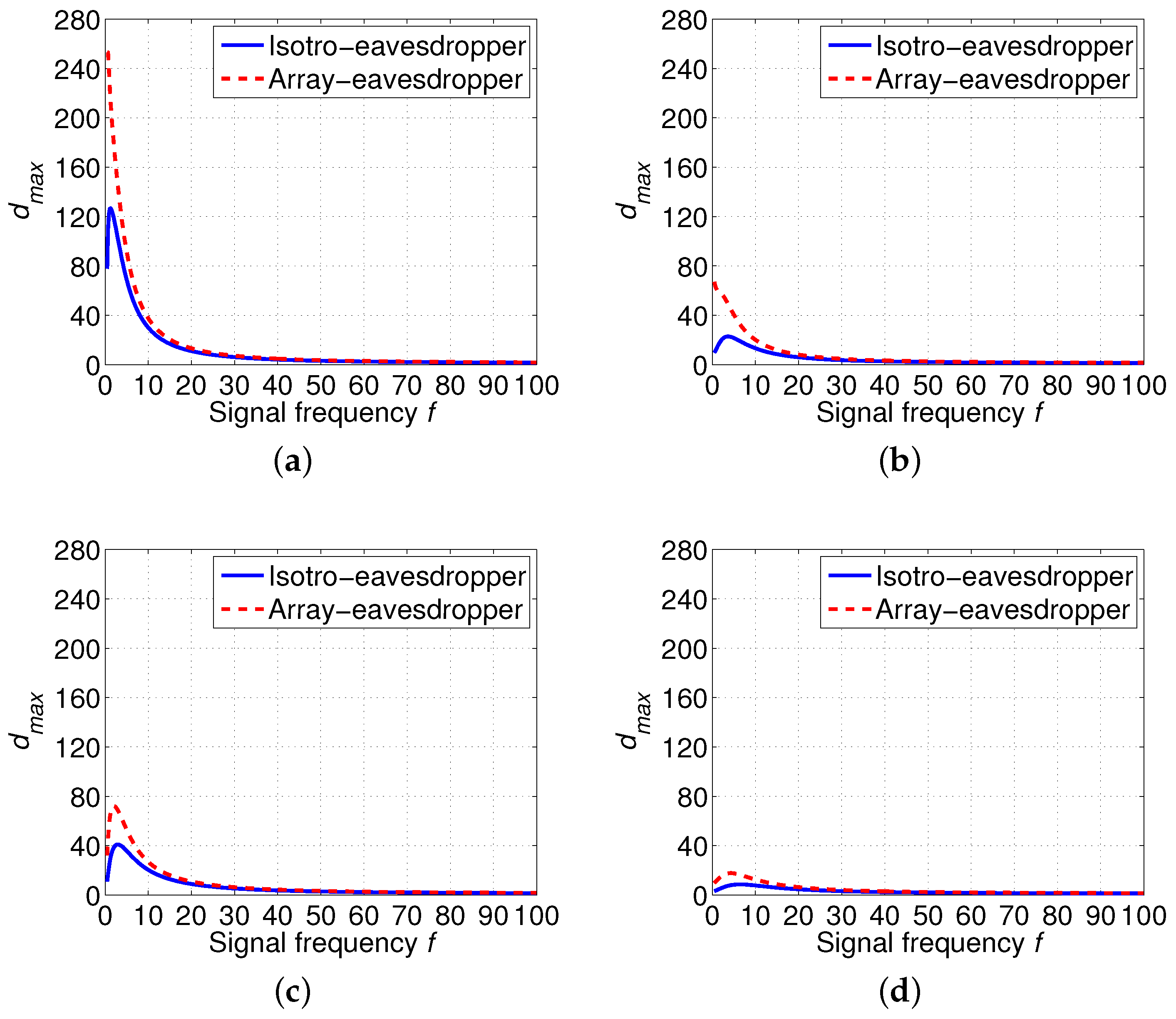
- We compare the eavesdropping probability of IUSNs and AUSNs. In particular, we find that the eavesdropping probability of AUSNs is lower than that of IUSNs, implying that using array hydrophones in UASNs can reduce the eavesdropping probability. We also find that an array eavesdropper has a higher eavesdropping probability than an isotropic eavesdropper in both IUSNs and AUSNs.
- We find that the eavesdropping probability heavily depends on the acoustic signal frequency, spreading factor, wind speed and the node density. Our results pave the way for designing a better protection mechanism in UASNs.
2. Underwater Acoustic Channel Model
2.1. Attenuation
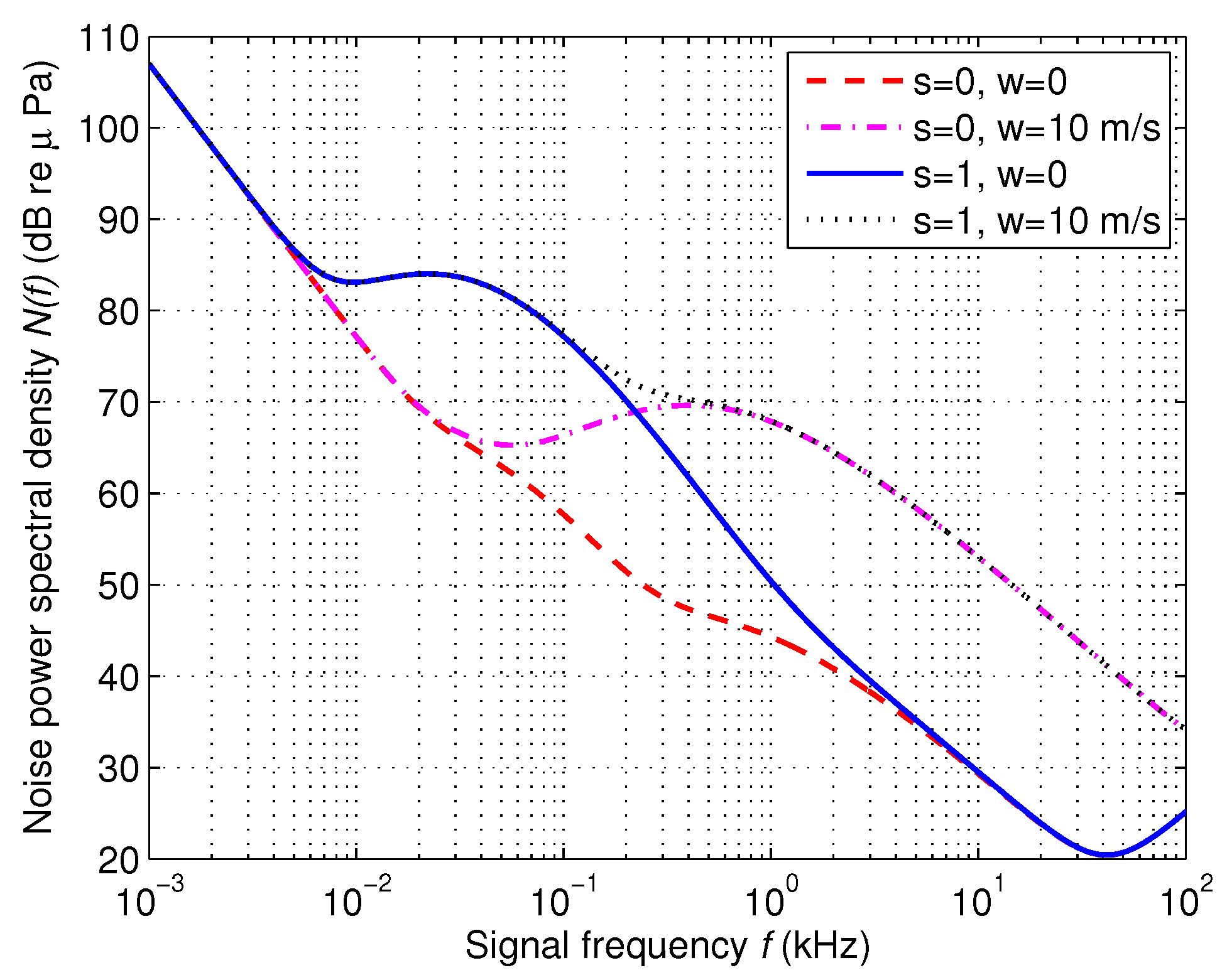
2.2. Ambient Noise
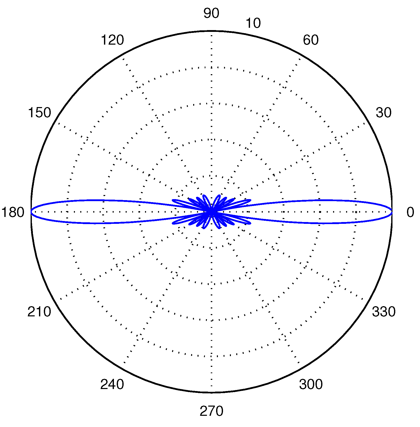
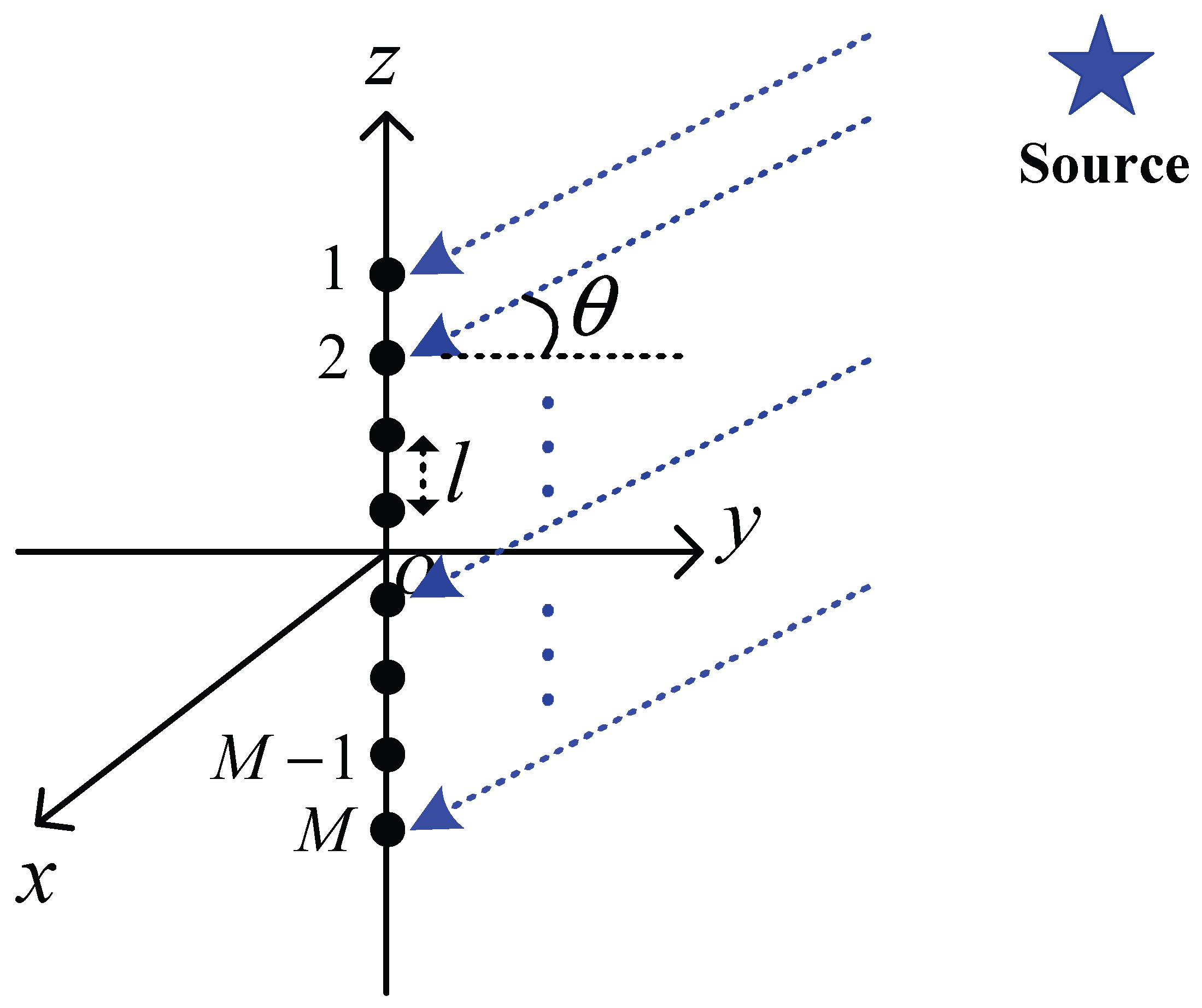
3. Transducers
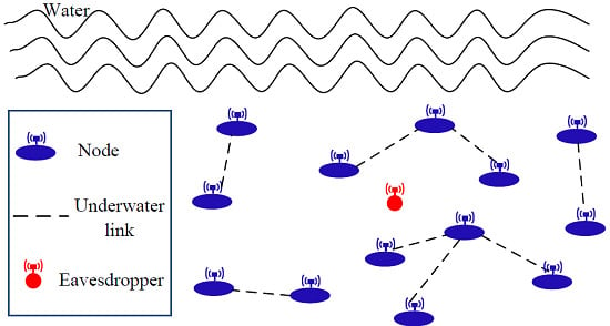
4. Analysis of Eavesdropping Attacks in UASNs
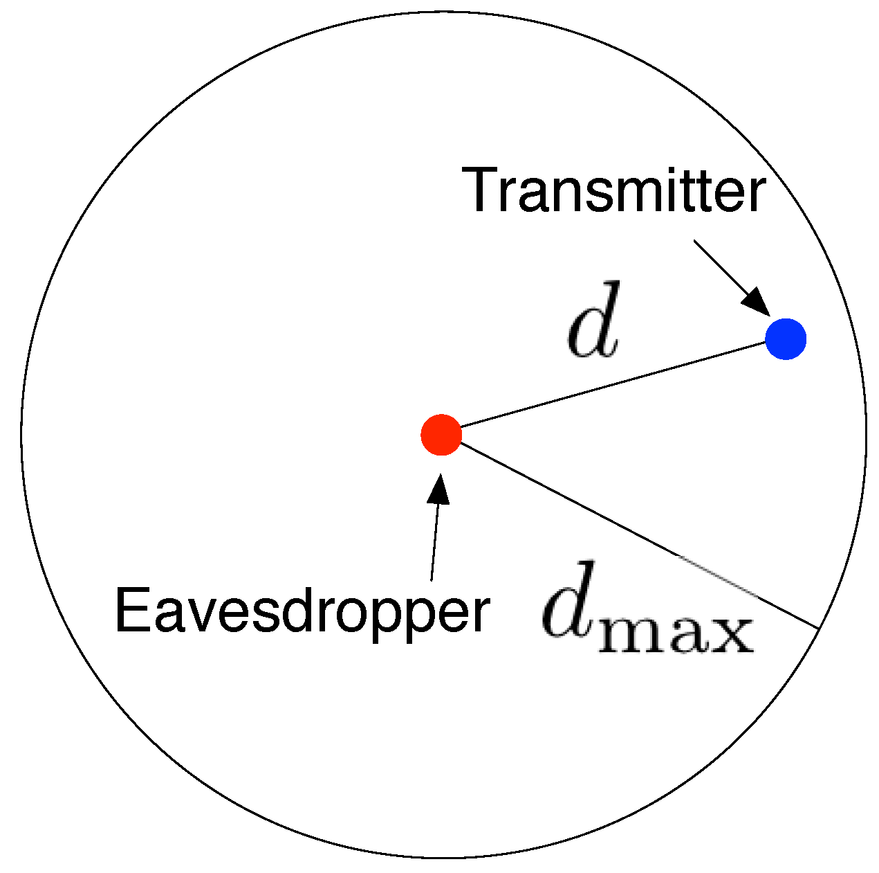
4.1. Link Criteria
4.2. Eavesdropping Success Condition
4.3. Eavesdropping Probability
5. Empirical Results
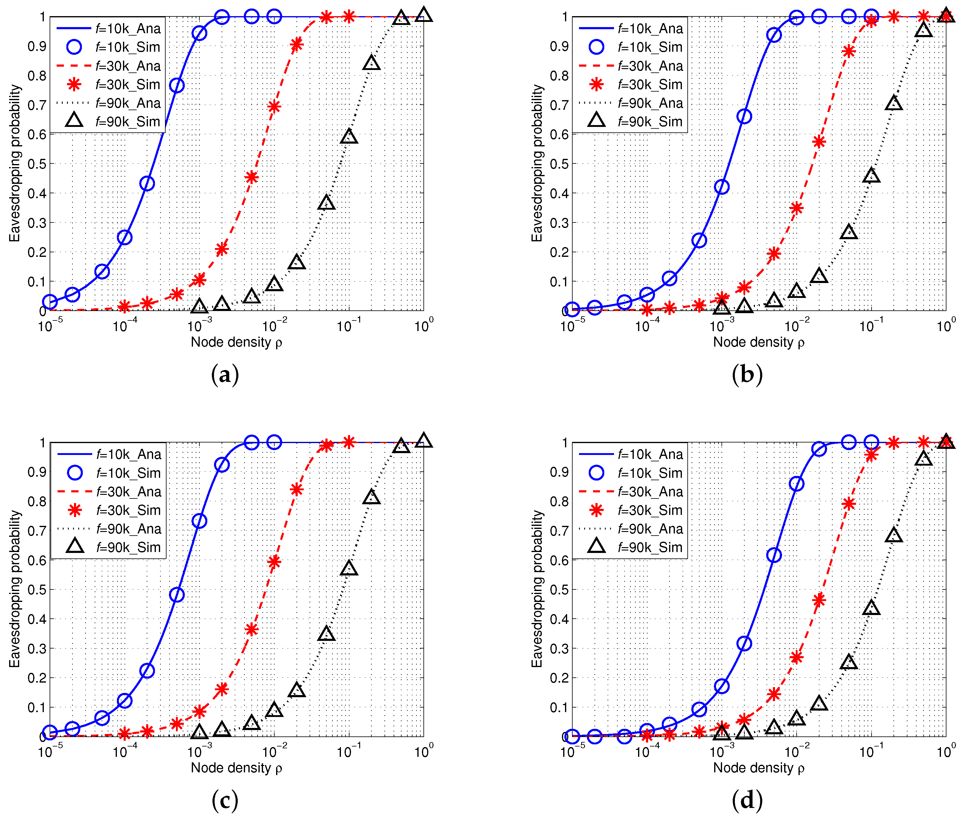
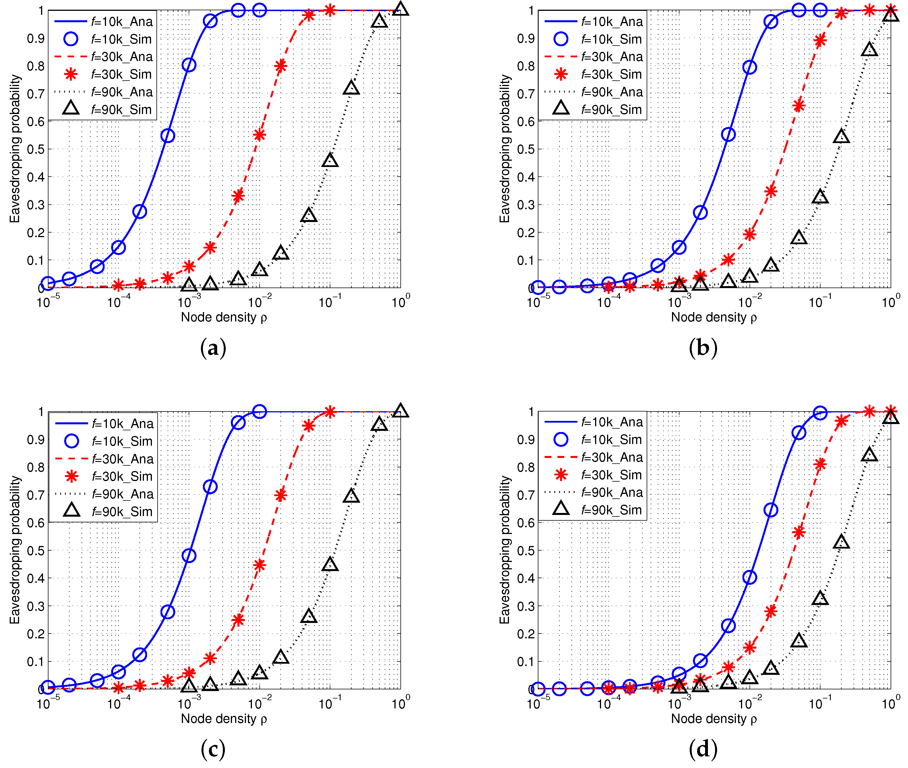
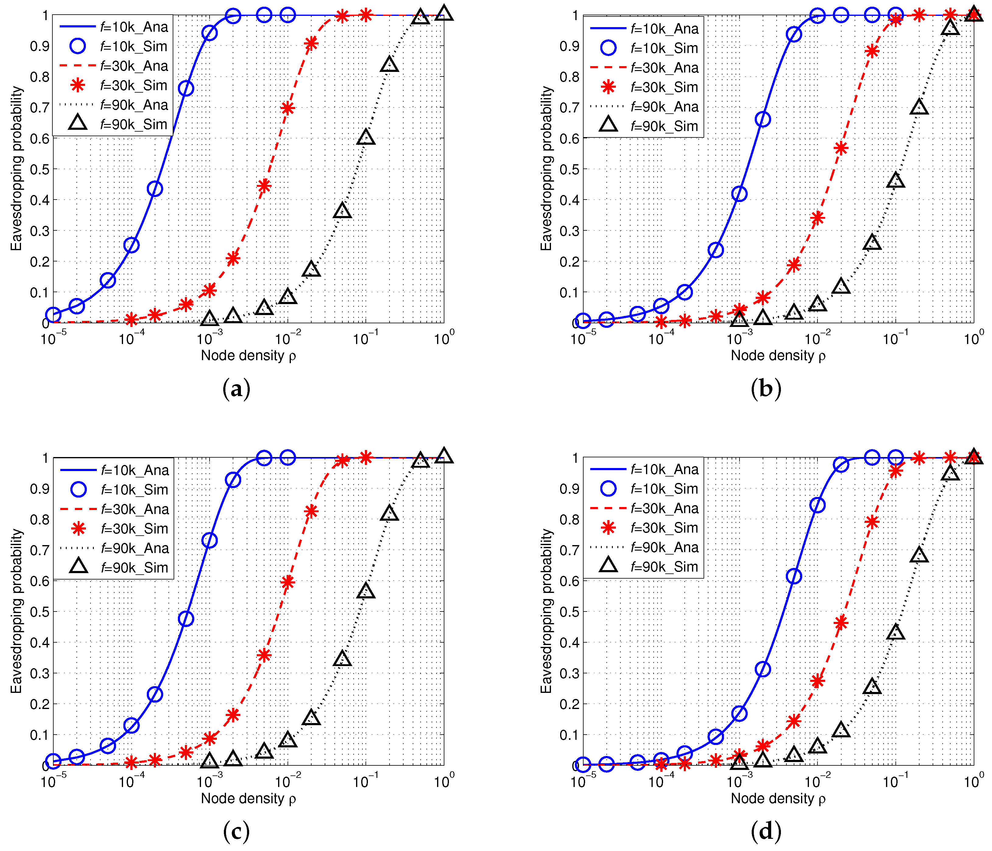
5.1. Eavesdropping Probability with an Isotropic Eavesdropper
5.1.1. Eavesdropping Probability in IUSNs
5.1.2. Eavesdropping Probability in AUSNs
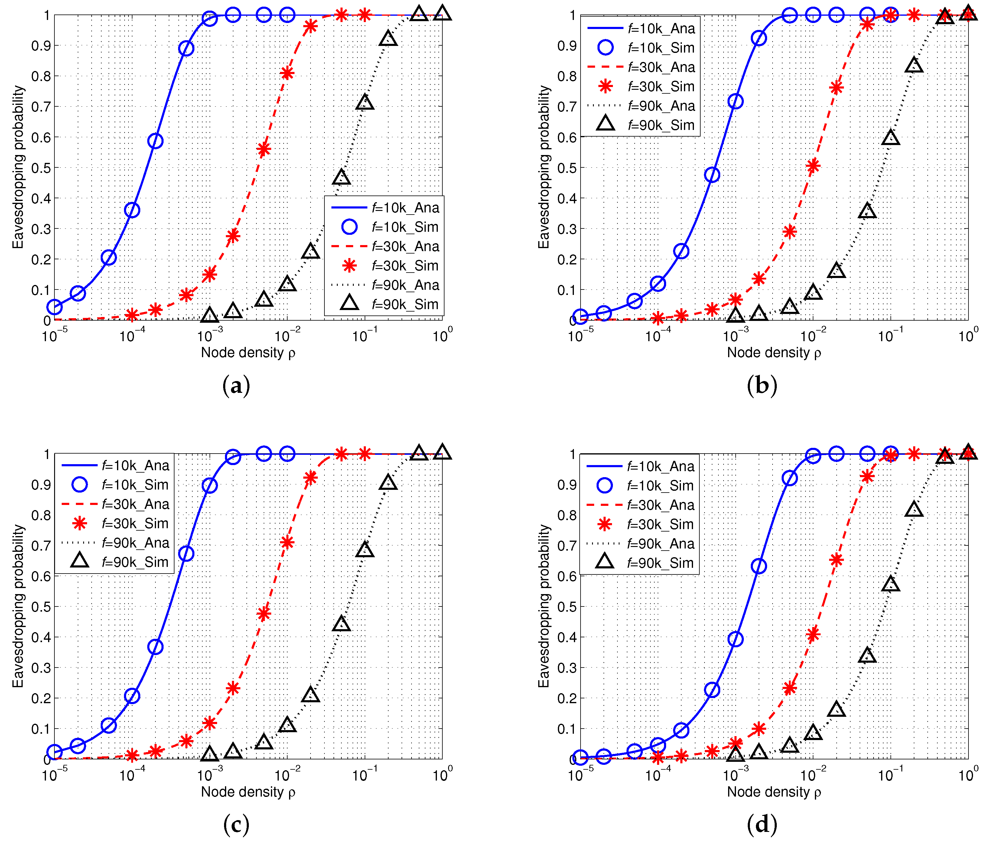
5.2. Eavesdropping Probability with an Array Eavesdropper
5.2.1. Eavesdropping Probability in IUSNs
5.2.2. Eavesdropping Probability in AUSNs
5.3. Comparison between an Isotropic Eavesdropper and an Array Eavesdropper
6. Conclusions
Acknowledgments
Author Contributions
Conflicts of Interest
References
- Han, G.; Jiang, J.; Sun, N.; Shu, L. Secure communication for underwater acoustic sensor networks. IEEE Commun. Mag. 2015, 53, 54–60. [Google Scholar] [CrossRef]
- Baggeroer, A.B. Acoustic Telemetry-An Overview. IEEE J. Ocean. Eng. 1984, 9, 229–235. [Google Scholar] [CrossRef]
- Heidemann, J.; Stojanovic, M.; Zorzi, M. Underwater sensor networks: Applications, advances and challenges. Philos. Trans. R. Soc. A 2012, 370, 158–175. [Google Scholar] [CrossRef] [PubMed]
- Zhang, W.; Stojanovic, M.; Mitra, U. Analysis of a Linear Multihop Underwater Acoustic Network. IEEE J. Ocean. Eng. 2010, 35, 961–970. [Google Scholar] [CrossRef]
- Lucani, D.; Medard, M.; Stojanovic, M. Capacity scaling laws for underwater networks. In Proceedings of the 42nd Asilomar Conference on Signals, Systems and Computers, Pacific Grove, CA, USA, 26–29 October 2008; pp. 2125–2129.
- Shin, W.Y.; Lucani, D.E.; Médard, M.; Stojanovic, M.; Tarokh, V. On the Effects of Frequency Scaling over Capacity Scaling in Underwater Networks—Part I: Extended Network Model. Wirel. Pers. Commun. 2013, 71, 1683–1700. [Google Scholar] [CrossRef]
- Shin, W.Y.; Lucani, D.E.; Médard, M.; Stojanovic, M.; Tarokh, V. On the Effects of Frequency Scaling over Capacity Scaling in Underwater Networks—Part II: Dense Network Model. Wirel. Pers. Commun. 2013, 71, 1701–1719. [Google Scholar] [CrossRef]
- Watanabe, S.; Kamiya, Y.; Umebayashi, K.; Suzuki, Y. A New Efficient and Robust MAC Protocol against Multipath Fading for Ad Hoc Networks. In Proceedings of the 19th Annual IEEE International Symposium on Personal, Indoor and Mobile Radio Communications (PIMRC’08), Cannes, France, 15–18 September 2008.
- Mandal, P.; De, S. New Reservation Multiaccess Protocols for Underwater Wireless Ad Hoc Sensor Networks. IEEE J. Ocean. Eng. 2015, 40, 277–291. [Google Scholar] [CrossRef]
- Ahmed, S.; Javaid, N.; Khan, F.A.; Durrani, M.Y.; Ali, A.; Shaukat, A.; Sandhu, M.M.; Khan, Z.A.; Qasim, U. Co-UWSN: Cooperative Energy-Efficient Protocol for Underwater WSNs. Int. J. Distrib. Sens. Netw. 2015, 2015. [Google Scholar] [CrossRef] [PubMed]
- Pompili, D.; Melodia, T.; Akyildiz, I. Distributed Routing Algorithms for Underwater Acoustic Sensor Networks. IEEE Trans. Wirel. Commun. 2010, 9, 2934–2944. [Google Scholar] [CrossRef]
- Rahman, R.H.; Benson, C.; Frater, M. Routing Protocols for Underwater Ad Hoc Networks. In Proceedings of the 2012 IEEE Oceans, Yeosu, Korea, 21–24 May 2012.
- Javaid, N.; Jafri, M.R.; Ahmed, S.; Jamil, M.; Khan, Z.A.; Qasim, U.; Al-Saleh, S.S. Delay-Sensitive Routing Schemes for Underwater Acoustic Sensor Networks. Int. J. Distrib. Sens. Netw. 2015. [Google Scholar] [CrossRef]
- Luo, Y.; Pu, L.; Zuba, M.; Peng, Z.; Cui, J.H. Challenges and Opportunities of Underwater Cognitive Acoustic Networks. IEEE Trans. Emerg. Top. Comput. 2014, 2, 198–211. [Google Scholar] [CrossRef]
- Ateniese, G.; Capossele, A.; Gjanci, P.; Petrioli, C.; Spaccini, D. SecFUN: Security Framework for Underwater acoustic sensor Networks. In Proceedings of the 2015 MTS/IEEE OCEANS, Genova, Italy, 18–21 May 2015.
- Lu, X.; Yonghua, Z. Modeling the Wormhole Attack in Underwater Sensor Network. In Proceedings of the 12th IEEE International Conference on Wireless Communications, Networking and Mobile Computing, Shanghai, China, 21–23 September 2012.
- Zuba, M.; Shi, Z.; Peng, Z.; Cui, J.H.; Zhou, S. Vulnerabilities of underwater acoustic networks to denial-of-service jamming attacks. Secur. Commun. Netw. 2015, 8, 2635–2645. [Google Scholar] [CrossRef]
- Anjum, F.; Mouchtaris, P. Security for Wireless Ad Hoc Networks, 1st ed.; Wiley-Interscience: Hoboken, NJ, USA, 2007. [Google Scholar]
- Wagner, D.; Schneier, B.; Kelsey, J. Cryptanalysis of the cellular message encryption algorithm. In Advances in Cryptology—CRYPTO ’97; Springer: Berlin/Heidelberg, Germany, 1997; Volume 1294, pp. 526–537. [Google Scholar]
- IEEE 802.11a-1999. In Specifications: High Speed Physical Layer in the 5 GHz Band; IEEE Standards Association: Piscataway, NJ, USA, 1999.
- IEEE 802.11i-2004. In Amendment 6: Medium Access Control (MAC) Security Enhancements; IEEE Standards Association: Piscataway, NJ, USA, 2004.
- Granjal, J.; Monteiro, E.; Silva, J. Security for the Internet of Things: A Survey of Existing Protocols and Open Research issues. IEEE Commun. Surv. Tutor. 2015, 17, 1294–1312. [Google Scholar] [CrossRef]
- Yick, J.; Mukherjee, B.; Ghosal, D. Wireless sensor network survey. Comput. Netw. 2008, 52, 2292–2330. [Google Scholar] [CrossRef]
- Kao, J.C.; Marculescu, R. Eavesdropping Minimization via Transmission Power Control in Ad-Hoc Wireless Networks. In Proceedings of the IEEE 2006 3rd Annual IEEE Communications Society on Sensor and Ad Hoc Communications and Networks, Reston, VA, USA, 28 September 2006; pp. 707–714.
- Raymond, D.R.; Midkiff, S.F. Denial-of-Service in Wireless Sensor Networks: Attacks and Defenses. IEEE Pervasive Comput. 2008, 7, 74–81. [Google Scholar] [CrossRef]
- Lu, X.; Wicker, F.; Lio, P.; Towsley, D. Security Estimation Model with Directional Antennas. In Proceedings of the 2008 IEEE Military Communications Conference, San Diego, CA, USA, 16–19 November 2008.
- Dai, H.N.; Li, D.; Wong, R.C.W. Exploring Security Improvement of Wireless Networks with Directional Antennas. In Proceedings of the IEEE 36th Conference on Local Computer Networks (LCN), Bonn, Germany, 4–7 October 2011.
- Wang, Q.; Dai, H.N.; Zhao, Q. Eavesdropping Security in Wireless Ad Hoc Networks with Directional Antennas. In Proceedings of the IEEE 2013 22nd Wireless and Optical Communication Conference, Chongqing, China, 16–18 May 2013; pp. 687–692.
- Dai, H.N.; Wang, Q.; Li, D.; Wong, R.C.W. On Eavesdropping Attacks in Wireless Sensor Networks with Directional Antennas. Int. J. Distrib. Sens. Netw. 2013, 2013. [Google Scholar] [CrossRef]
- Li, X.; Xu, J.; Dai, H.N.; Zhao, Q.; Cheang, C.F.; Wang, Q. On Modeling Eavesdropping Attacks in Wireless Networks. J. Comput. Sci. 2015, 11, 196–204. [Google Scholar] [CrossRef]
- Sankararaman, S.; Abu-Affash, K.; Efrat, A.; Eriksson-Bique, S.D.; Polishchuk, V.; Ramasubramanian, S.; Segal, M. Optimization Schemes for Protective Jamming. In Proceedings of the Thirteenth ACM International Symposium on Mobile Ad Hoc Networking and Computing, Hilton Head, SC, USA, 11–14 June 2012; pp. 65–74.
- Kim, Y.S.; Tague, P.; Lee, H.; Kim, H. A Jamming Approach to Enhance Enterprise Wi-Fi Secrecy Through Spatial Access Control. Wirel. Netw. 2015, 21, 2631–2647. [Google Scholar] [CrossRef]
- He, X.; Khisti, A.; Yener, A. MIMO Multiple Access Channel With an Arbitrarily Varying Eavesdropper: Secrecy Degrees of Freedom. IEEE Trans. Inf. Theory 2013, 59, 4733–4745. [Google Scholar]
- Zou, Y.; Champagne, B.; Zhu, W.P.; Hanzo, L. Relay-Selection Improves the Security-Reliability Trade-Off in Cognitive Radio Systems. IEEE Trans. Commun. 2015, 63, 215–228. [Google Scholar] [CrossRef]
- Li, X.; Dai, H.N.; Zhao, Q. An Analytical Model on Eavesdropping Attacks in Wireless Networks. In Proceedings of the IEEE International Conference on Communication Systems (ICCS), Macau, 19–21 November 2014; pp. 538–542.
- Emokpae, L.; Younis, M. Throughput Analysis for Shallow Water Communication Utilizing Directional Antennas. IEEE J. Sel. Areas Commun. 2012, 30, 1006–1018. [Google Scholar] [CrossRef]
- Coates, R. Underwater Acoustic Systems; Palgrave Macmillan: London, UK, 1990. [Google Scholar]
- Stojanovic, M. On the Relationship Between Capacity and Distance in an Underwater Acoustic Communication Channel. In Proceedings of the First ACM International Workshop on Underwater Networks (WUWNet), Los Angeles, CA, USA, 29 September 2006; pp. 41–47.
- Hodges, R.P. Underwater Acoustics: Analysis, Design and Performance of Sonars, 1st ed.; Wiley: Hoboken, NJ, USA, 2010. [Google Scholar]
- Bettstetter, C. On the Connectivity of Ad Hoc Networks. Comput. J. 2004, 47, 432–447. [Google Scholar] [CrossRef]
- Won, T.H.; Park, S.J. Design and Implementation of an Omni-Directional Underwater Acoustic Micro-Modem Based on a Low-Power Micro-Controller Unit. Sensors 2012, 12, 2309–2323. [Google Scholar] [CrossRef] [PubMed]


© 2016 by the authors; licensee MDPI, Basel, Switzerland. This article is an open access article distributed under the terms and conditions of the Creative Commons Attribution (CC-BY) license (http://creativecommons.org/licenses/by/4.0/).
Share and Cite
Wang, Q.; Dai, H.-N.; Li, X.; Wang, H.; Xiao, H. On Modeling Eavesdropping Attacks in Underwater Acoustic Sensor Networks. Sensors 2016, 16, 721. https://doi.org/10.3390/s16050721
Wang Q, Dai H-N, Li X, Wang H, Xiao H. On Modeling Eavesdropping Attacks in Underwater Acoustic Sensor Networks. Sensors. 2016; 16(5):721. https://doi.org/10.3390/s16050721
Chicago/Turabian StyleWang, Qiu, Hong-Ning Dai, Xuran Li, Hao Wang, and Hong Xiao. 2016. "On Modeling Eavesdropping Attacks in Underwater Acoustic Sensor Networks" Sensors 16, no. 5: 721. https://doi.org/10.3390/s16050721