
Frequency Optimization for Enhancement of Surface Defect Classification Using the Eddy Current Technique


Abstract
: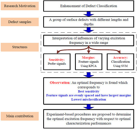
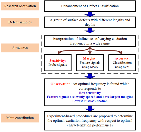
1. Introduction
2. Methodology
2.1. Kernel PCA
2.2. Support Vector Machine
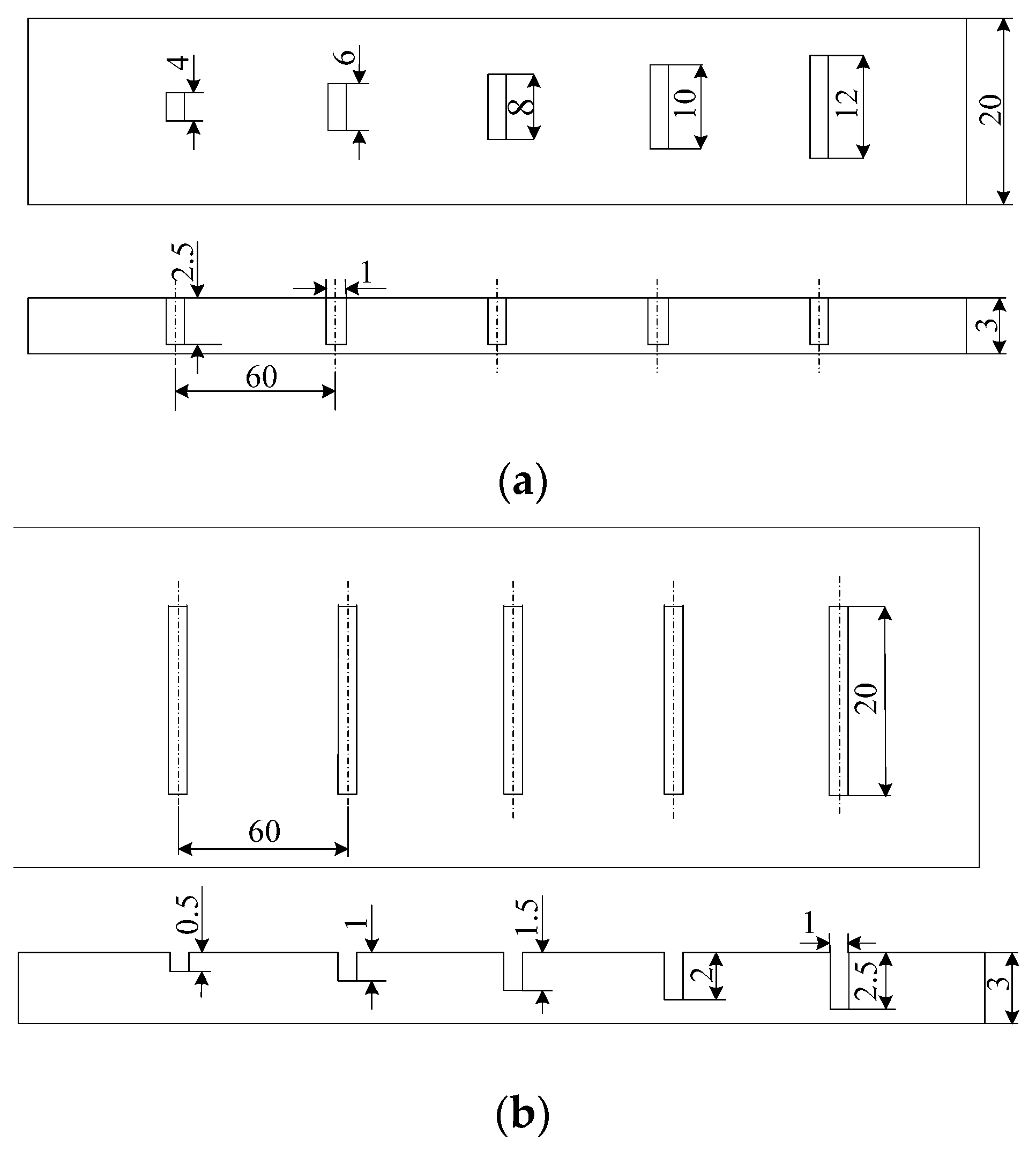
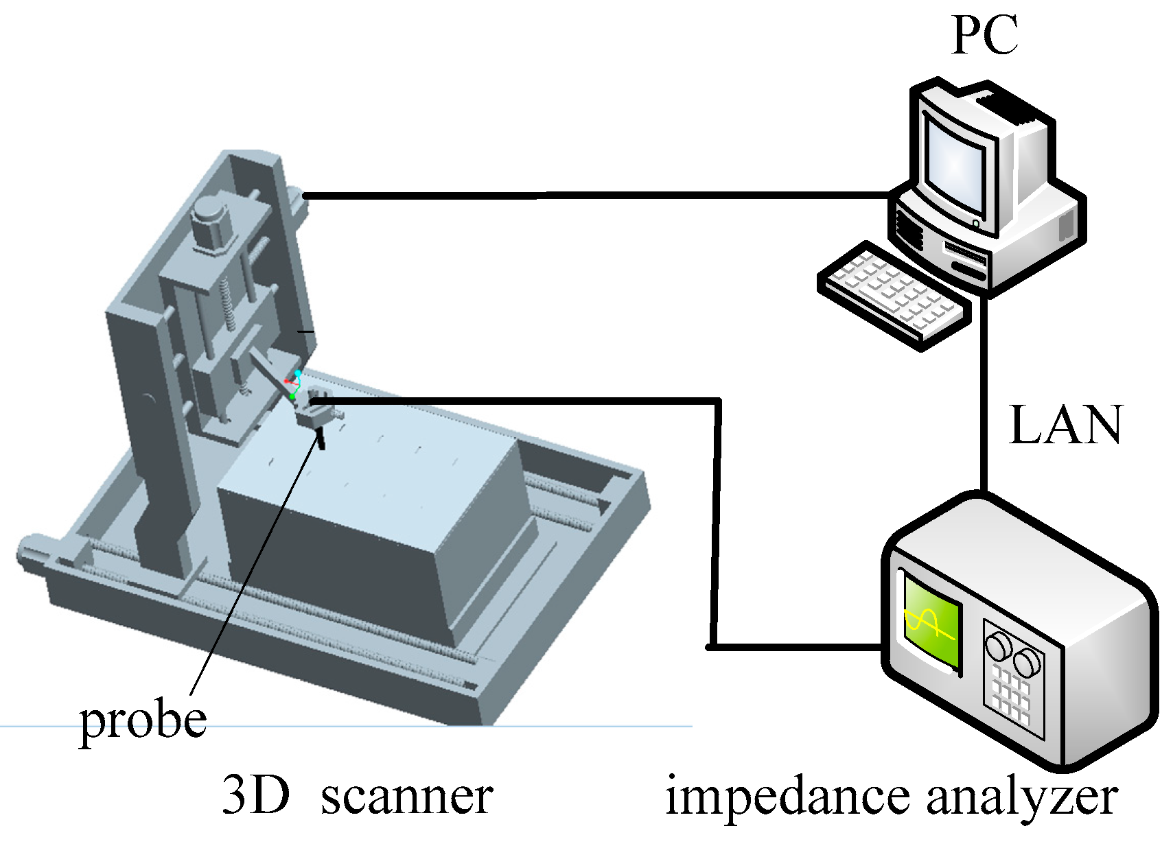
3. Experimental Setup and Specimens
4. Results and Discussion
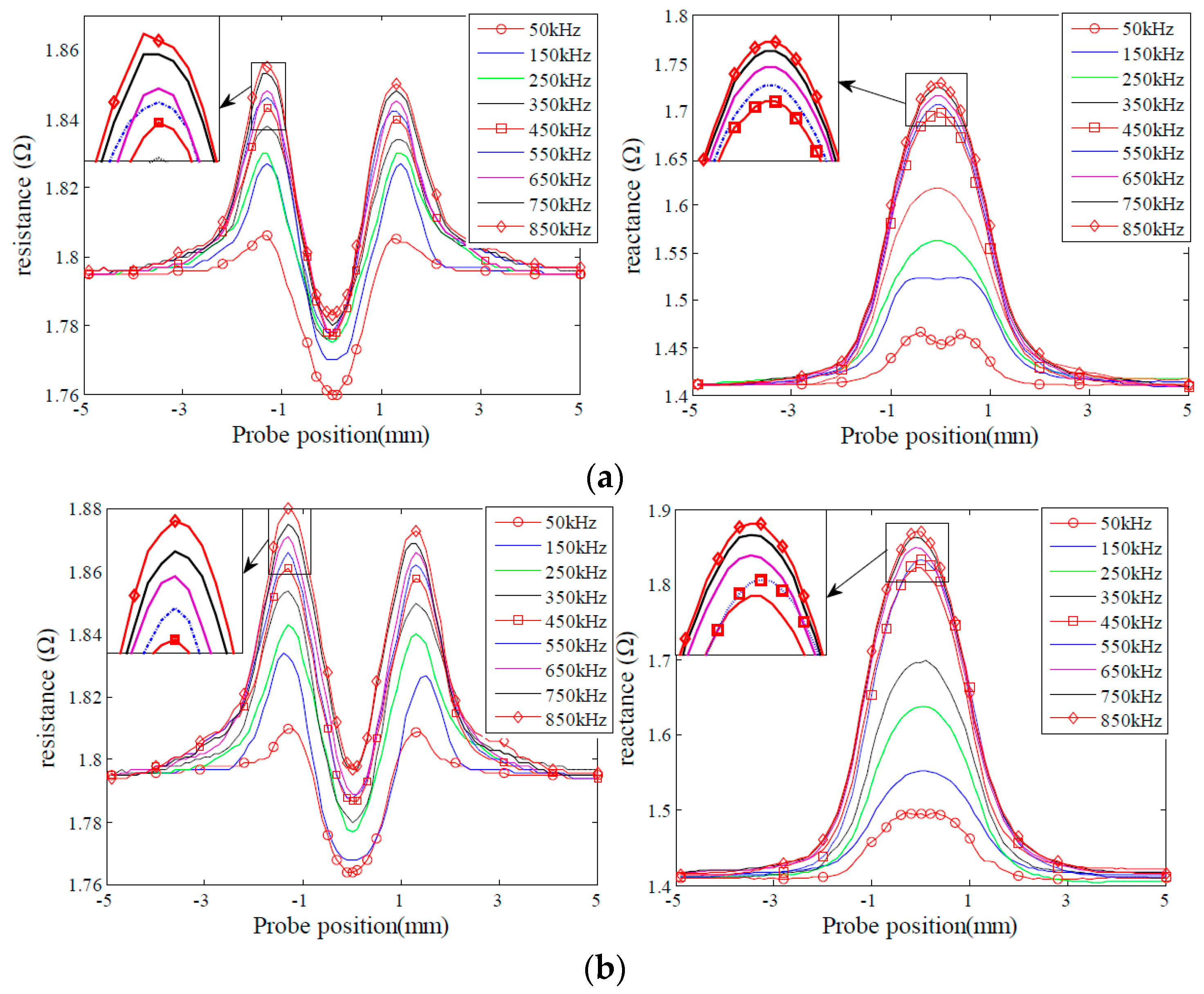
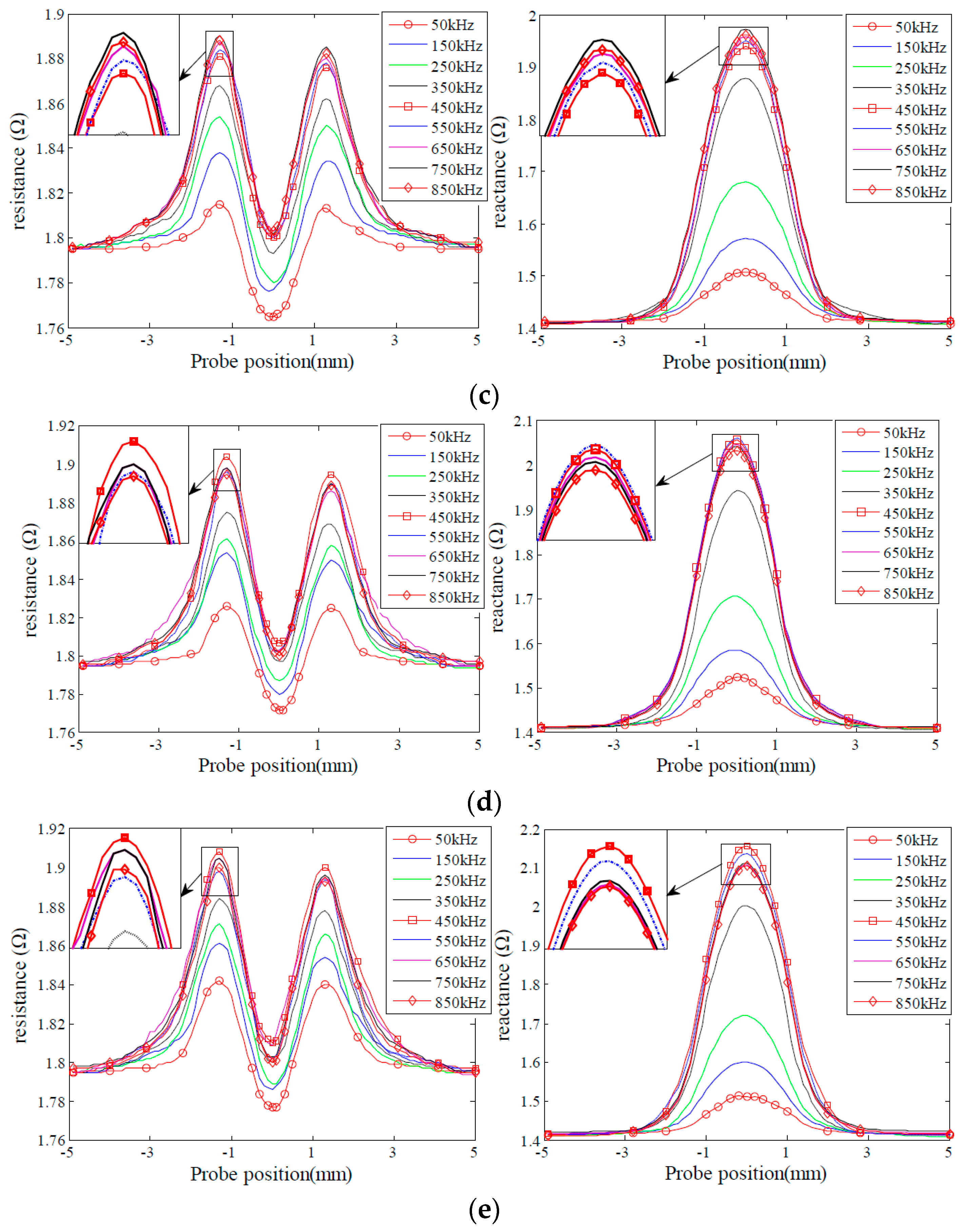
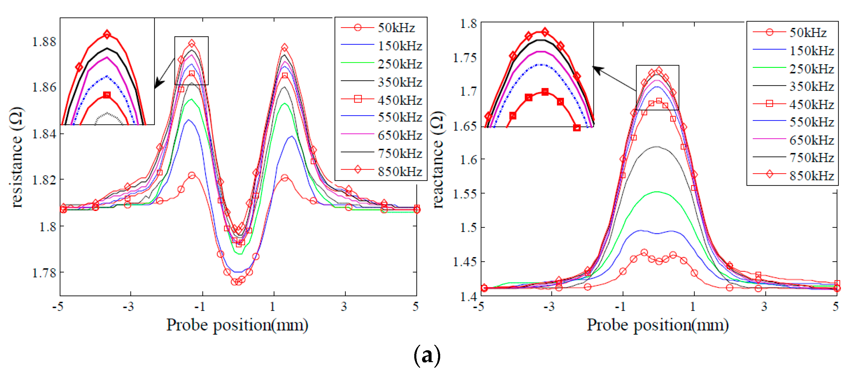
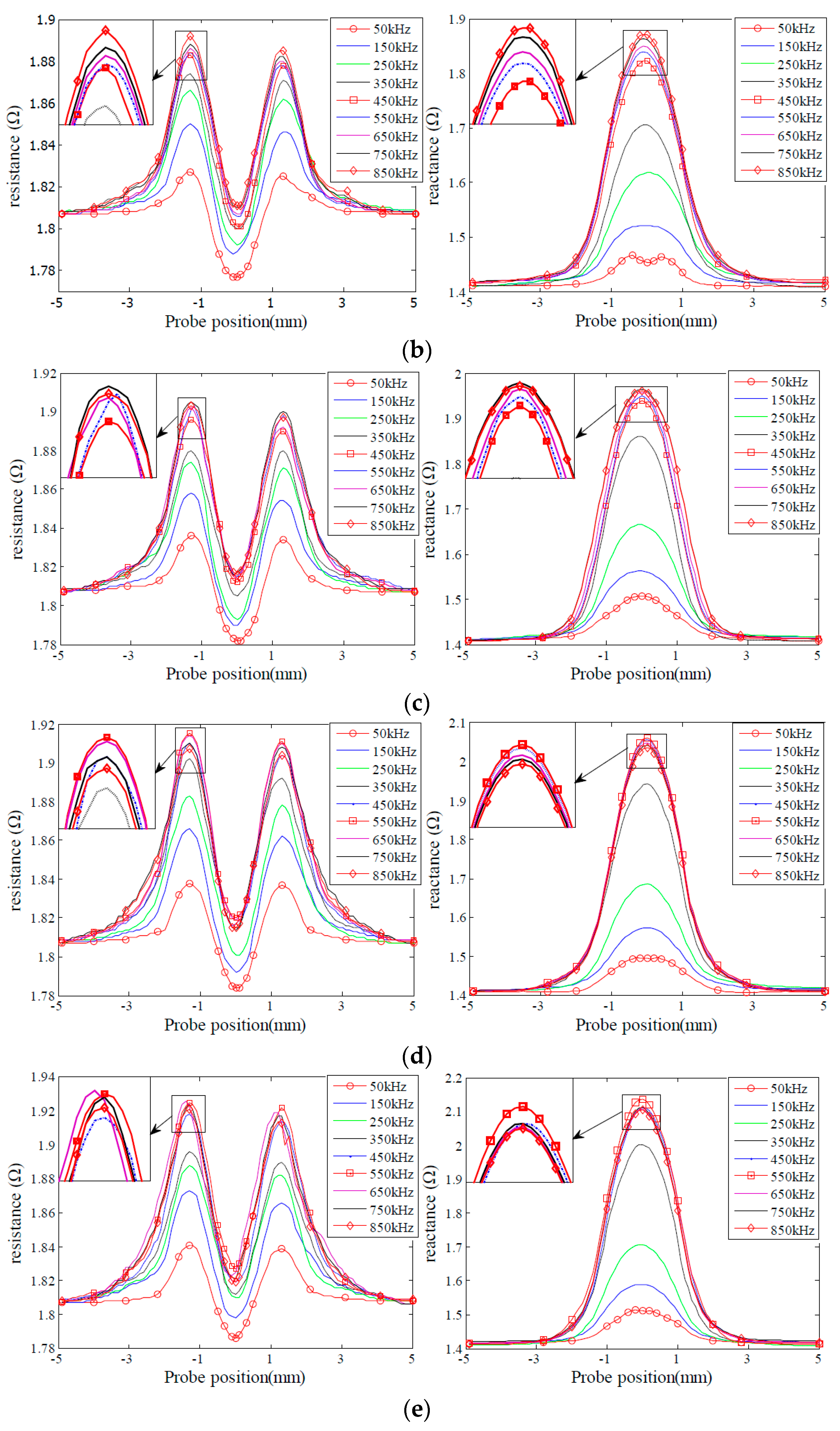
4.1. Effect on Detection Sensitivity
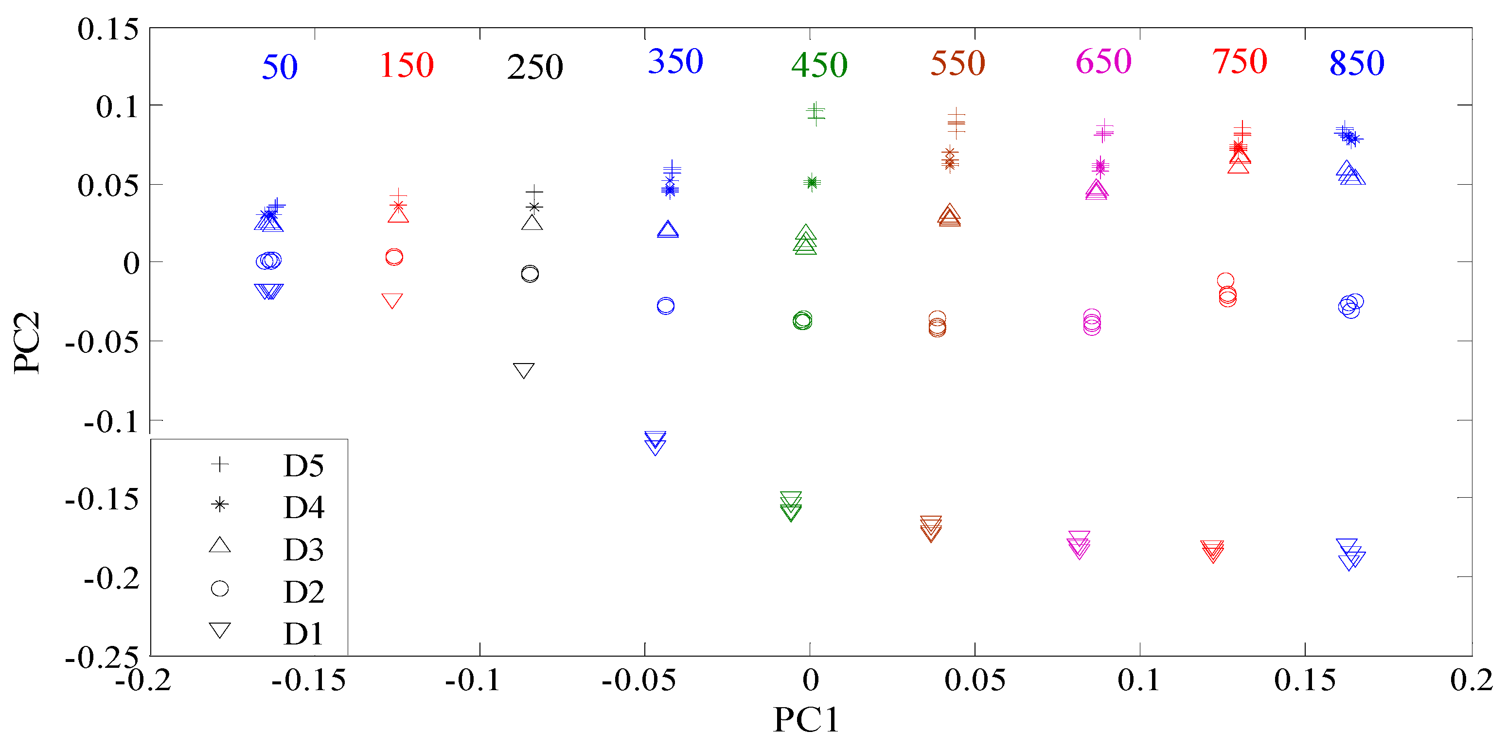
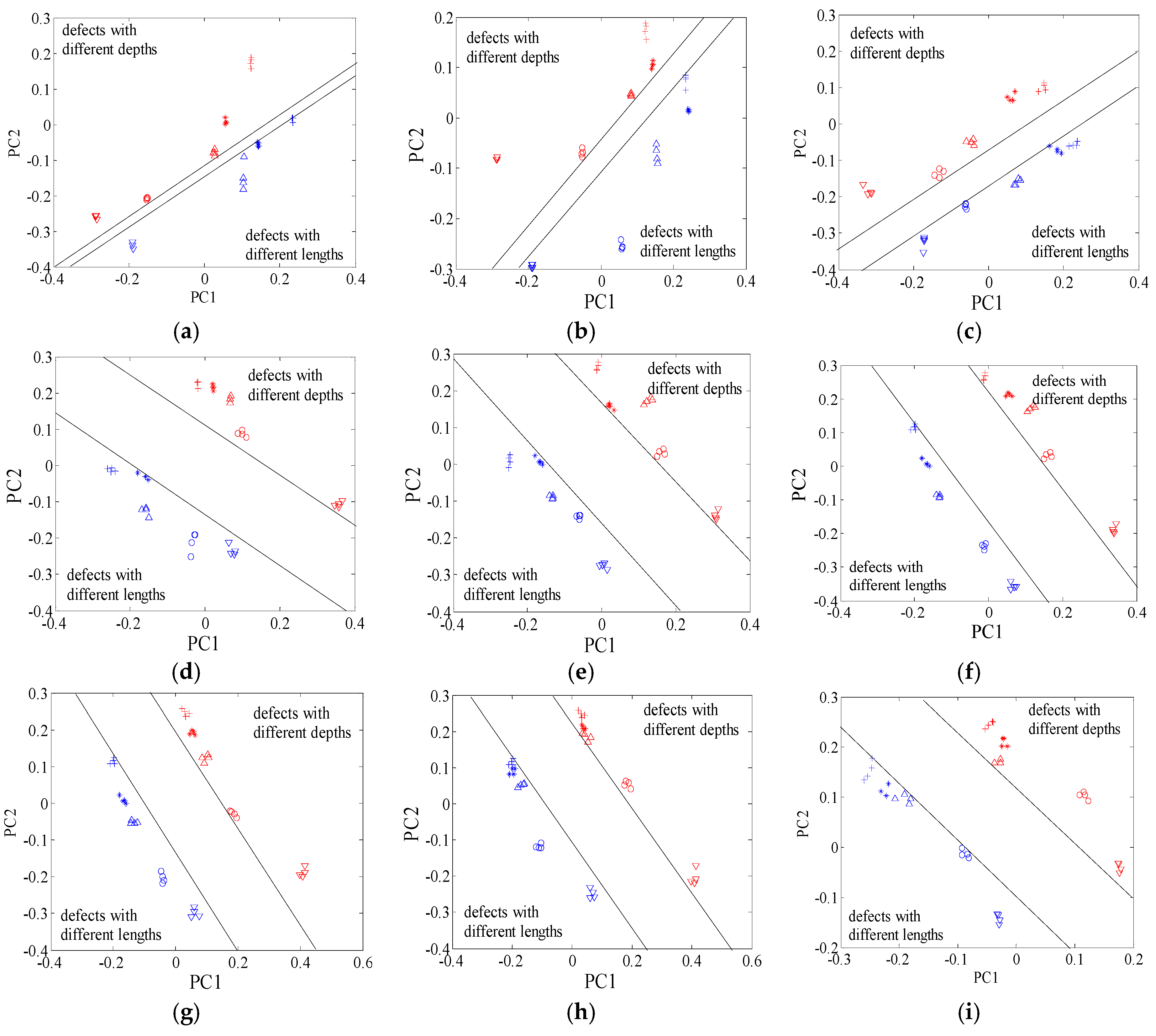
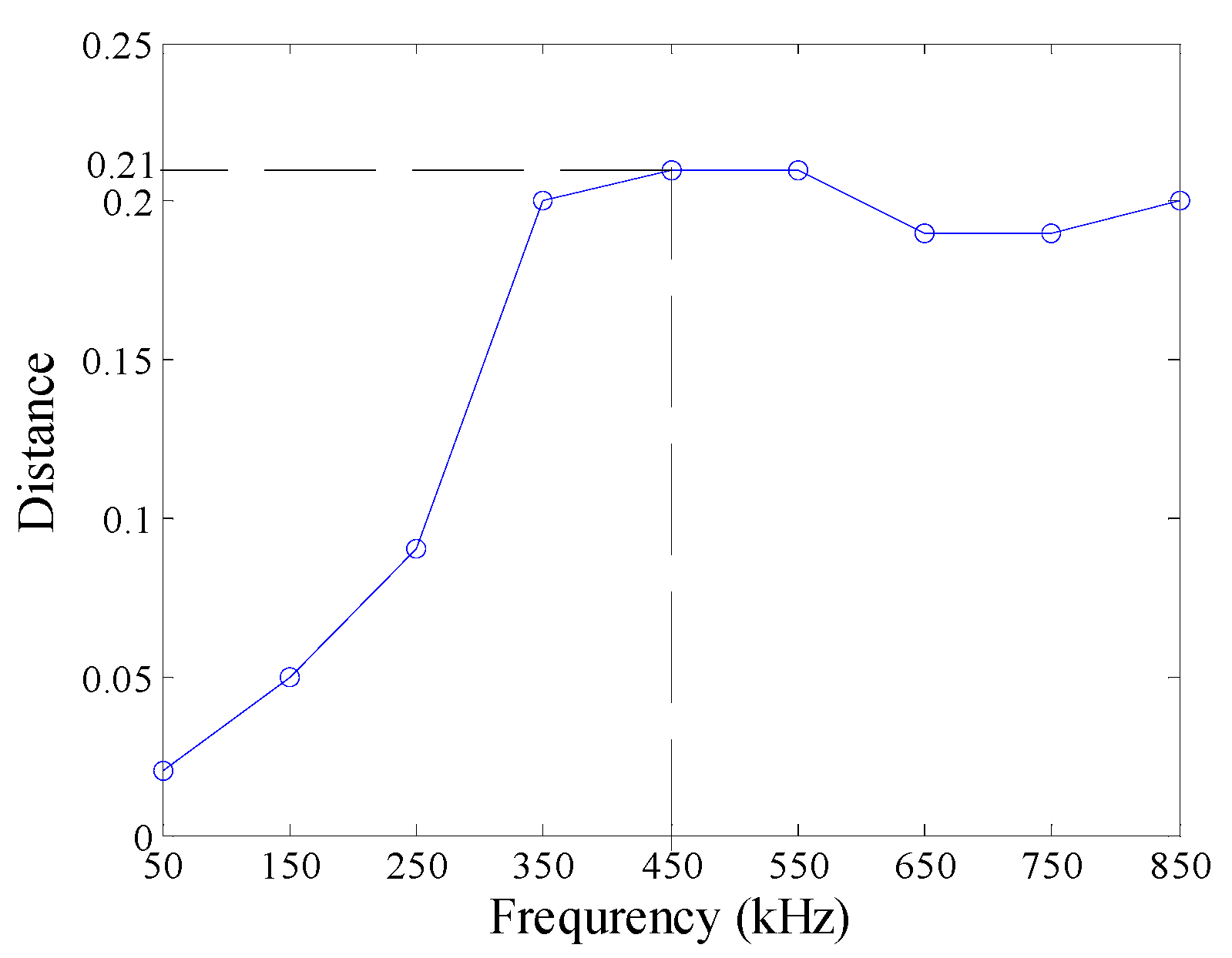
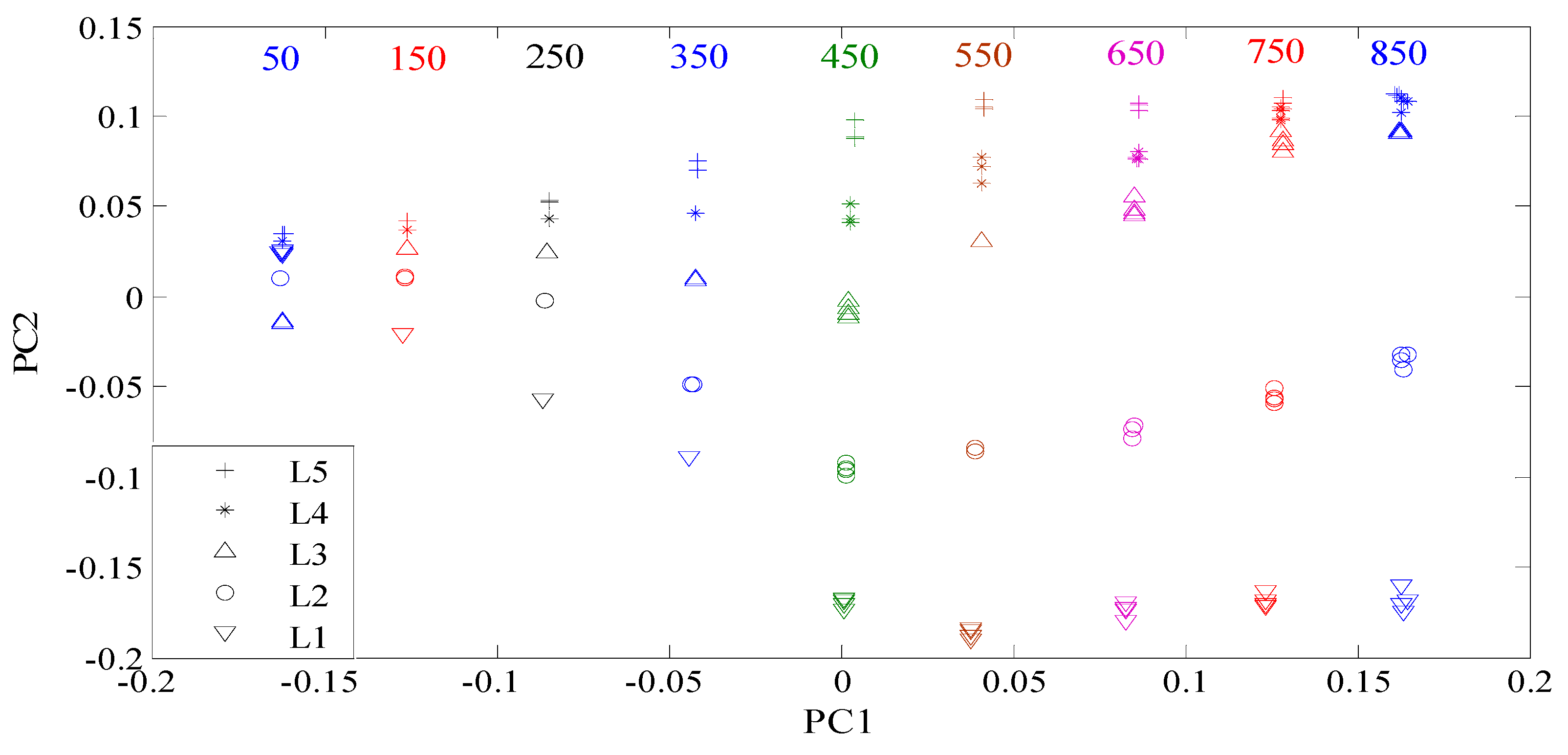
4.2. Effect on the Contrast of Defect Features
4.3. Effect on Classification Accuracy
4.4. Discussions and Limitation
- (1)
- Determine the range of the defects to be identified before inspections;
- (2)
- Manufacture a sample defect with a maximum depth and length;
- (3)
- Observe probe signals when excitation frequency is adjusted continuously until maximum signals are retrieved for the fabricated sample defect;
- (4)
- The optimal frequency should be equal to the frequency corresponding to the observed maximum probe signals.
5. Conclusions
Acknowledgments
Author Contributions
Conflicts of Interest
References
- Xie, R.; Chen, D.; Pan, M.; Tian, W.; Wu, X.; Zhou, W.; Tang, Y. Fatigue crack length sizing using a novel flexible eddy current sensor array. Sensors 2015, 15, 32138–32151. [Google Scholar] [CrossRef] [PubMed]
- Li, Y.; Yan, B.; Li, D.; Li, Y.L.; Zhou, D.Q. Gradient-field pulsed eddy current probes for imaging of hidden corrosion in conductive structures. Sens. Actuator A Phys. 2016, 238, 251–265. [Google Scholar] [CrossRef]
- Alcantara, N.; Silva, F.; Guimarães, M.; Pereira, M. Corrosion assessment of steel bars used in reinforced concrete structures by means of eddy current testing. Sensors 2016, 16, 4409–4418. [Google Scholar] [CrossRef] [PubMed]
- Guarneri, G.; Pipa, D.; Junior, F.; Arruda, L.; Zibetti, M. A sparse reconstruction algorithm for ultrasonic images in nondestructive testing. Sensors 2015, 15, 9324–9343. [Google Scholar] [CrossRef] [PubMed]
- Felice, M.V.; Velichko, A.; Wilcox, P.D. Accurate depth measurement of small surface-breaking cracks using an ultrasonic array post-processing technique. NDT&E Int. 2014, 68, 105–112. [Google Scholar]
- Zou, Y.R.; Du, D.; Bao, B.H. Automatic weld defect detection method based on Kalman filtering for real-time radiographic in section of spiral pipe. NDT&E Int. 2015, 72, 1–9. [Google Scholar]
- Lindgren, E. Detection, 3-D positioning and sizing of small probe detects using digital radiograph and tracking. EURASIP J. Adv. Sig. Process. 2014. [Google Scholar] [CrossRef]
- Chen, X.; Hou, D.B.; Zhao, L.; Huang, P.J.; Zhang, G.X. Study on defect classification in multi-layer structures based on Fisher linear discriminate analysis by using pulsed eddy current technique. NDT&E Int. 2014, 67, 46–54. [Google Scholar]
- Saludes-Rodil, S.; Baeyens, E.; Rodríguez-Juan, C. Unsupervised classification of surface defects in wire rod production obtained by eddy current sensors. Sensors 2015, 15, 10100–10117. [Google Scholar] [CrossRef] [PubMed]
- Rocha, T.J.; Ramos, H.G.; Ribeiro, A.L.; Pasadas, D.J. Magnetic sensors assessment in velocity induced eddy current testing. Sens. Actuator A Phys. 2015, 228, 55–61. [Google Scholar] [CrossRef]
- Rosado, L.S.; Janeiro, F.M. Defect characterization with eddy current testing using nonlinear-regression feature extraction and artificial neural networks. IEEE Trans. Instrum. Meas. 2013, 62, 1207–1214. [Google Scholar] [CrossRef]
- Yusa, N.; Huang, H.Y.; Miya, K. Numerical evaluation of the ill-posedness of eddy current problems to size real cracks. NDT&E Int. 2007, 40, 185–191. [Google Scholar]
- Li, Y.; Udpa, L.; Udpa, S.S. Three-dimensional defect reconstruction from eddy-current NDE signals using a genetic local search algorithm. IEEE Trans. Magn. 2004, 40, 410–417. [Google Scholar] [CrossRef]
- Yusa, N.; Hashizume, H.; Urayama, R.; Uchimoto, T.; Takagi, T.; Sato, K. An arrayed uniform eddy current probe design for crack monitoring and sizing of surface breaking cracks with the aid of a computational inversion technique. NDT& E Int. 2014, 61, 29–34. [Google Scholar]
- Fan, M.B.; Cao, B.H.; Yang, P.P.; Li, W.; Tian, G.Y. Elimination of liftoff effect using a model-based method for eddy current characterization of a plate. NDT&E Int. 2015, 74, 66–71. [Google Scholar]
- Tian, G.Y.; Sophian, A. Reduction of lift-off effects for pulsed eddy current NDT. NDT&E Int. 2005, 38, 319–324. [Google Scholar]
- Tian, G.Y.; He, Y.Z.; Adewale, I. Research on spectral response of pulsed eddy current and NDE applications. Sens. Actuator A Phys. 2013, 189, 313–320. [Google Scholar] [CrossRef]
- Yu, Y.T.; Yan, Y.; Wang, F.; Tian, G.Y.; Zhang, D.J. An approach to reduce lift-off noise in pulsed eddy current nondestructive technology. NDT&E Int. 2015, 63, 1–6. [Google Scholar]
- Chen, G.M.; Li, W.; Wang, Z.X. Structural optimization of 2-D array probe for alternatingcurrent field measurement. NDT&E Int. 2007, 40, 455–461. [Google Scholar]
- Chady, T.; Sikora, R. Optimization of eddy-current sensor for multifrequency systems. IEEE Trans. Magn. 2003, 39, 1313–1316. [Google Scholar] [CrossRef]
- Chen, Z.M.; Miya, K. A new approach for optimal design of eddy current testing probes. J. Nondestruct. Eval. 1998, 17, 105–116. [Google Scholar] [CrossRef]
- Joubert, P.Y.; Vourch, E.; Thomas, V. Experimental validation of an eddy current probe dedicated to the multi-frequency imaging of bore holes. Sens. Actuator A Phys. 2012, 185, 132–138. [Google Scholar] [CrossRef]
- Rosado, L.S.; Gonzalez, J.C.; Santos, T.G.; Ramos, P.M.; Piedade, M. Geometric optimization of a differential planar eddy currents probe for nondestructive testing. Sens. Actuator A Phys. 2013, 197, 96–105. [Google Scholar] [CrossRef]
- Horan, P.F.; Underhill, P.R.; Krause, T.W. Real time pulsed eddy current detection of cracks in F/A-18 inner wing spar using discriminant separation of modified principal components analysis score. IEEE Sens. J. 2014, 14, 171–177. [Google Scholar] [CrossRef]
- Ye, B.; Huang, P.J.; Fan, M.B.; Gong, X.; Hou, D.B.; Zhang, G.X.; Zhou, Z.K. Automatic classification of eddy current signals based on kernel methods. Nondestruct. Test. Eval. 2009, 24, 19–37. [Google Scholar] [CrossRef]
- Cheng, L.; Gao, B.; Tian, G.Y. Impact Damage detection and identification using eddy current pulsed thermography through integration of PCA and ICA. IEEE Sens. J. 2014, 14, 1655–1663. [Google Scholar] [CrossRef]
- Jia, P.F.; Tian, F.C.; He, Q.H.; Fan, S. Feature extraction of wound infection data for electronic nose based on a novel weight KPCA. Sens. Actuator B Chem. 2014, 201, 555–566. [Google Scholar] [CrossRef]
- Bernieri, A.; Betta, G.; Ferrigno, L.; Laracca, M.; Mastrostefano, S. Multifrequency excitation and support vector machine regressor for ECT defect characterization. IEEE Trans. Instrum. Meas. 2014, 63, 1271–1280. [Google Scholar] [CrossRef]
- Liu, B.L.; Huang, P.J.; Hou, D.B.; Chen, X.; Zhang, G.X. Application of Hilbert–Huang transform for defect recognition in pulsed eddy current testing. Nondestruct. Test. Eval. 2015, 30, 233–251. [Google Scholar] [CrossRef]
- Li, W.; Chen, G.M.; Li, W.Y.; Li, Z.; Liu, F. Analysis of the inducing frequency of a U-shaped ACFM system. NDT&E Int. 2011, 44, 324–328. [Google Scholar]
- Pereira, D.; Clarke, T. Modeling and design optimization of an eddy current sensor for superficial and subsuperficial crack detection in inconel claddings. IEEE Sens. J. 2015, 12, 1287–1292. [Google Scholar] [CrossRef]
- Biju, N.; Ganesan, N.; Krishnamurthy, C.V.; Balasubramaniam, K. Frequency optimization for eddy current thermography. NDT&E Int. 2009, 42, 415–420. [Google Scholar]
- Biju, N.; Ganesan, N.; Krishnamurthy, C.V.; Balasubramaniam, K. Optimum frequency variations with coil geometry and defects in tone burst eddy current thermography. Insight 2013, 55, 504–509. [Google Scholar] [CrossRef]
- Yin, W.L.; Peyton, A.J. Thickness measurement of non-magnetic plates using multi-frequency eddy current sensors. NDT&E Int. 2007, 40, 43–48. [Google Scholar]
- Kim, K.I.; Jung, K.; Kim, H.J. Face recognition using kernel principal component analysis. IEEE Signal. Proc. Lett. 2002, 9, 40–42. [Google Scholar]
- Hoffmann, H. Kernel PCA for novelty detection. Pattern Recog. 2007, 40, 863–874. [Google Scholar] [CrossRef]
- Hsu, C.W.; Lin, C.J. A comparison of methods for multiclass support vector machines. IEEE Trans. Neur. Netw. 2002, 13, 415–425. [Google Scholar]
- Chang, C.C.; Lin, C.J. LIBSVM: A library for support vector machines. ACM Trans. Intel. Syst. Technol. 2011, 3, 1–27. [Google Scholar] [CrossRef]
- Zhu, C.M.; Gao, D.Q. Improved multi-kernel classification machine with Nyström approximation technique. Pattern Recog. 2015, 48, 1490–1509. [Google Scholar] [CrossRef]
- Kuo, B.C.; Ho, H.H.; Li, C.H.; Hung, C.C.; Taur, J.S. A kernel-based feature selection method for SVM with RBF kernel for hyperspectral image classification. IEEE J. STARS 2014, 7, 317–326. [Google Scholar]
- Burrascano, P.; Carpentieri, M.; Pirani, A.; Ricci, M. Galois sequences in the non-destructive evaluation of metallic materials. Meas. Sci. Technol. 2006, 17, 2973–2979. [Google Scholar] [CrossRef]
- Betta, G.; Ferrigno, L.; Laracca, M.; Burrascano, P.; Ricci, M.; Silipigni, G. An experimental comparison of multi-frequency and chirp excitations for eddy current testing on thin defects. Measurement 2015, 63, 207–220. [Google Scholar] [CrossRef]
- Hamanaka, S.; Marinova, I.; Saito, Y.; Ohuch, M.; Kojima, T. Enhance the flat ∞ coil sensibility by multi-frequency convolution strategy. In Proceedings of the 20th International Workshop on Electromagnetic Nondestructive Evaluation, Sendai, Japan, 21–23 September 2015.
- Abidin, I.; Tian, G.Y.; Wilson, J.; Yang, S.X.; Almond, D. Quantitative evaluation of angular defects by pulsed eddy current thermography. NDT&E Int. 2010, 43, 537–546. [Google Scholar]
- Mukriz, I.; Tian, G.Y.; Li, Y. 3D transient magnetic field mapping for angular slots in aluminium. Insight 2009, 51, 21–24. [Google Scholar] [CrossRef]


| Defects | Length (mm) | Width (mm) | Depth (mm) | |
|---|---|---|---|---|
| different lengths (Sample 1) | L1 | 4 | 1 | 2.5 |
| L2 | 6 | |||
| L3 | 8 | |||
| L4 | 10 | |||
| L5 | 12 | |||
| different depths (Sample 2) | D1 | 20 | 1 | 0.5 |
| D2 | 1.0 | |||
| D3 | 1.5 | |||
| D4 | 2.0 | |||
| D5 | 2.5 | |||
| Defect | 50 kHz | 150 kHz | 250 kHz | 350 kHz | 450 kHz | 550 kHz | 650 kHz | 750 kHz | 850 kHz |
|---|---|---|---|---|---|---|---|---|---|
| D1 | 100% | 100% | 100% | 100% | 100% | 100% | 100% | 100% | 100% |
| D2 | 100% | 100% | 100% | 100% | 100% | 100% | 100% | 100% | 100% |
| D3 | 80% | 100% | 100% | 100% | 100% | 100% | 90% | 70% | 90% |
| D4 | 60% | 70% | 100% | 90% | 100% | 100% | 100% | 80% | 60% |
| D5 | 60% | 60% | 100% | 100% | 100% | 100% | 100% | 70% | 70% |
| L1 | 100% | 100% | 100% | 100% | 100% | 100% | 100% | 100% | 100% |
| L2 | 100% | 100% | 100% | 100% | 100% | 100% | 100% | 100% | 100% |
| L3 | 90% | 100% | 100% | 90% | 100% | 100% | 100% | 90% | 80% |
| L4 | 60% | 70% | 100% | 100% | 100% | 100% | 100% | 70% | 80% |
| L5 | 60% | 60% | 90% | 100% | 100% | 100% | 100% | 60% | 60% |
| Total | 88% | 92% | 96% | 100% | 100% | 100% | 96% | 92% | 92% |
| Classifier | Accuracy | ||||||||
|---|---|---|---|---|---|---|---|---|---|
| 50 kHz | 150 kHz | 250 kHz | 350 kHz | 450 kHz | 550 kHz | 650 kHz | 750 kHz | 850 kHz | |
| PCA-ANN | 90% | 93% | 95% | 96% | 95% | 97% | 94% | 93% | 92% |
| PCA-SVM | 88% | 88% | 92% | 96% | 100% | 100% | 96% | 92% | 88% |
| KPCA-ANN | 93% | 95% | 97% | 98% | 98% | 98% | 98% | 96% | 95% |
| KPCA-SVM | 88% | 92% | 96% | 100% | 100% | 100% | 96% | 92% | 92% |
© 2016 by the authors; licensee MDPI, Basel, Switzerland. This article is an open access article distributed under the terms and conditions of the Creative Commons Attribution (CC-BY) license (http://creativecommons.org/licenses/by/4.0/).
Share and Cite
Fan, M.; Wang, Q.; Cao, B.; Ye, B.; Sunny, A.I.; Tian, G. Frequency Optimization for Enhancement of Surface Defect Classification Using the Eddy Current Technique. Sensors 2016, 16, 649. https://doi.org/10.3390/s16050649
Fan M, Wang Q, Cao B, Ye B, Sunny AI, Tian G. Frequency Optimization for Enhancement of Surface Defect Classification Using the Eddy Current Technique. Sensors. 2016; 16(5):649. https://doi.org/10.3390/s16050649
Chicago/Turabian StyleFan, Mengbao, Qi Wang, Binghua Cao, Bo Ye, Ali Imam Sunny, and Guiyun Tian. 2016. "Frequency Optimization for Enhancement of Surface Defect Classification Using the Eddy Current Technique" Sensors 16, no. 5: 649. https://doi.org/10.3390/s16050649