
In situ Stiffness Adjustment of AFM Probes by Two Orders of Magnitude


Abstract
:
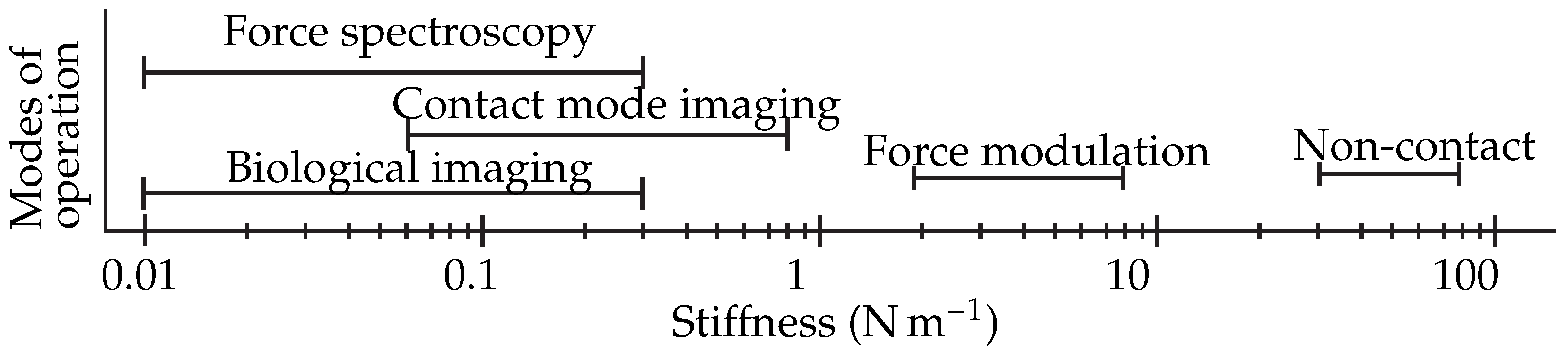
1. Introduction
2. Modeling
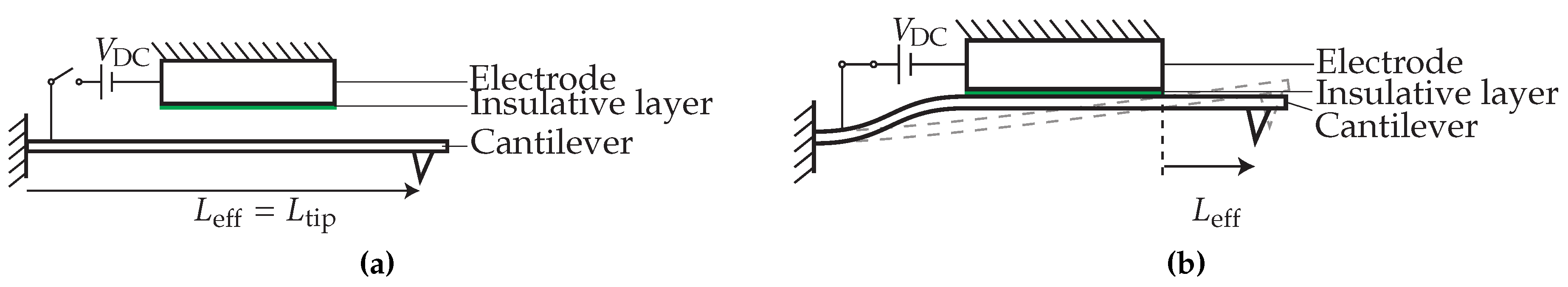
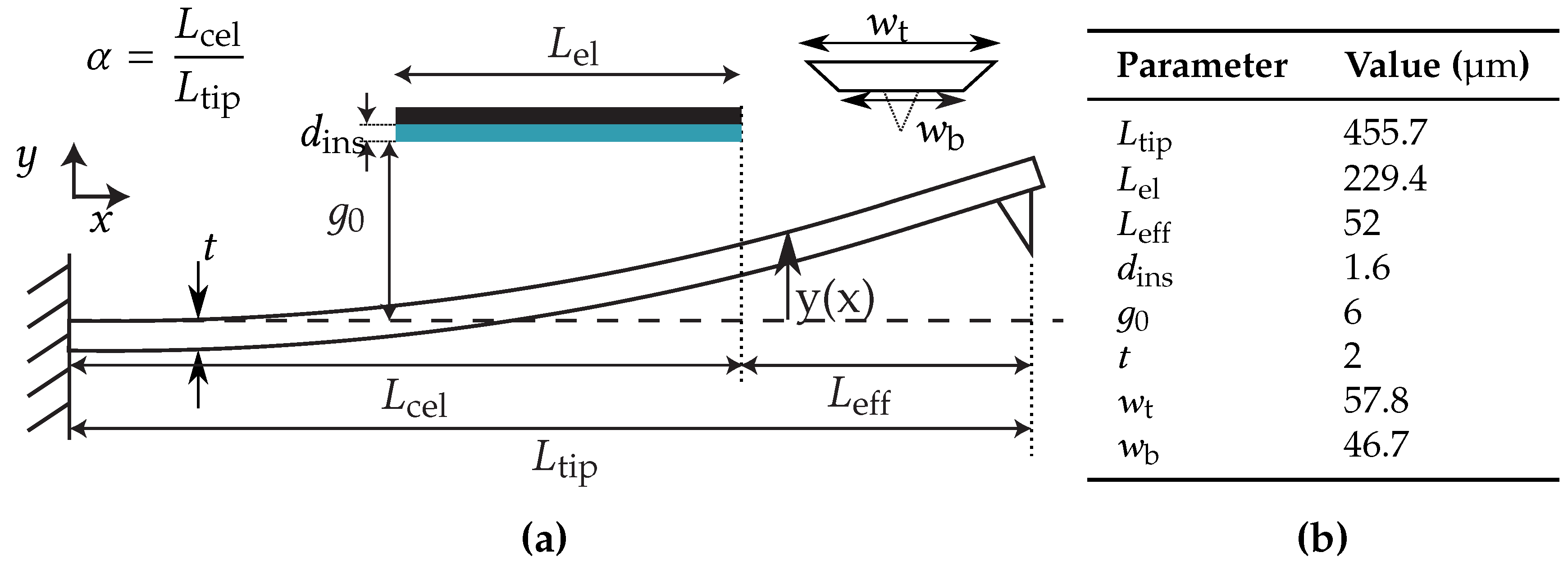
2.1. Analytical Model
2.2. FEM Model
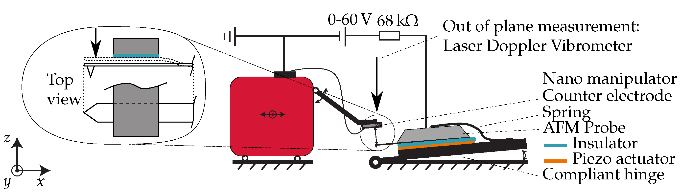
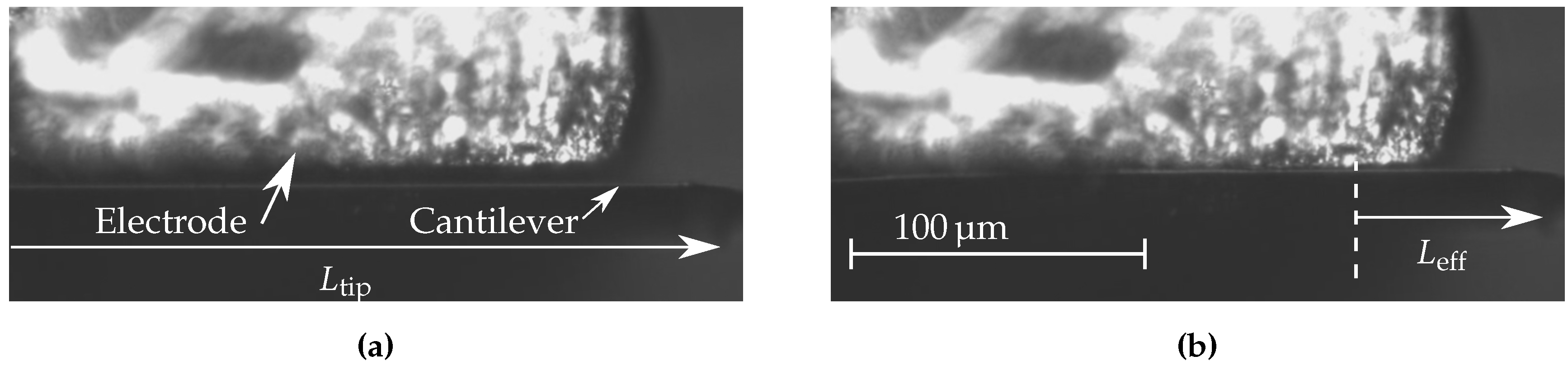
2.3. Experimental Setup
3. Results
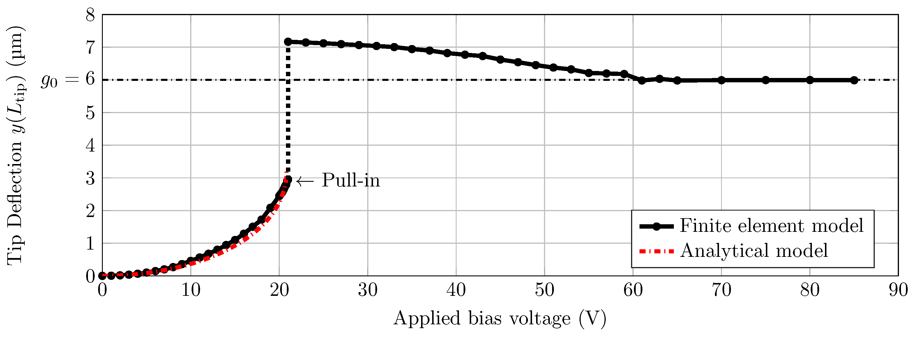
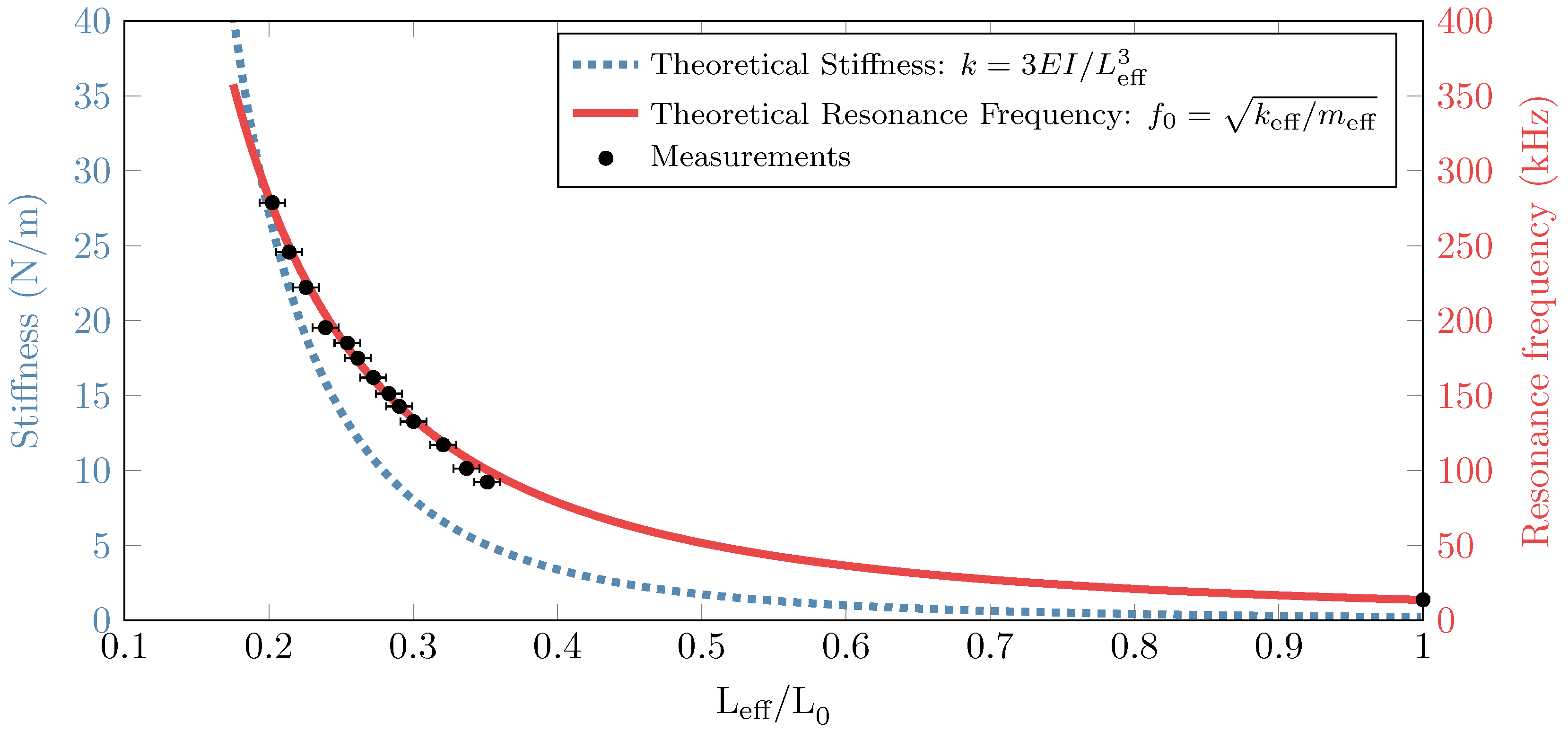
3.1. Modeling Results
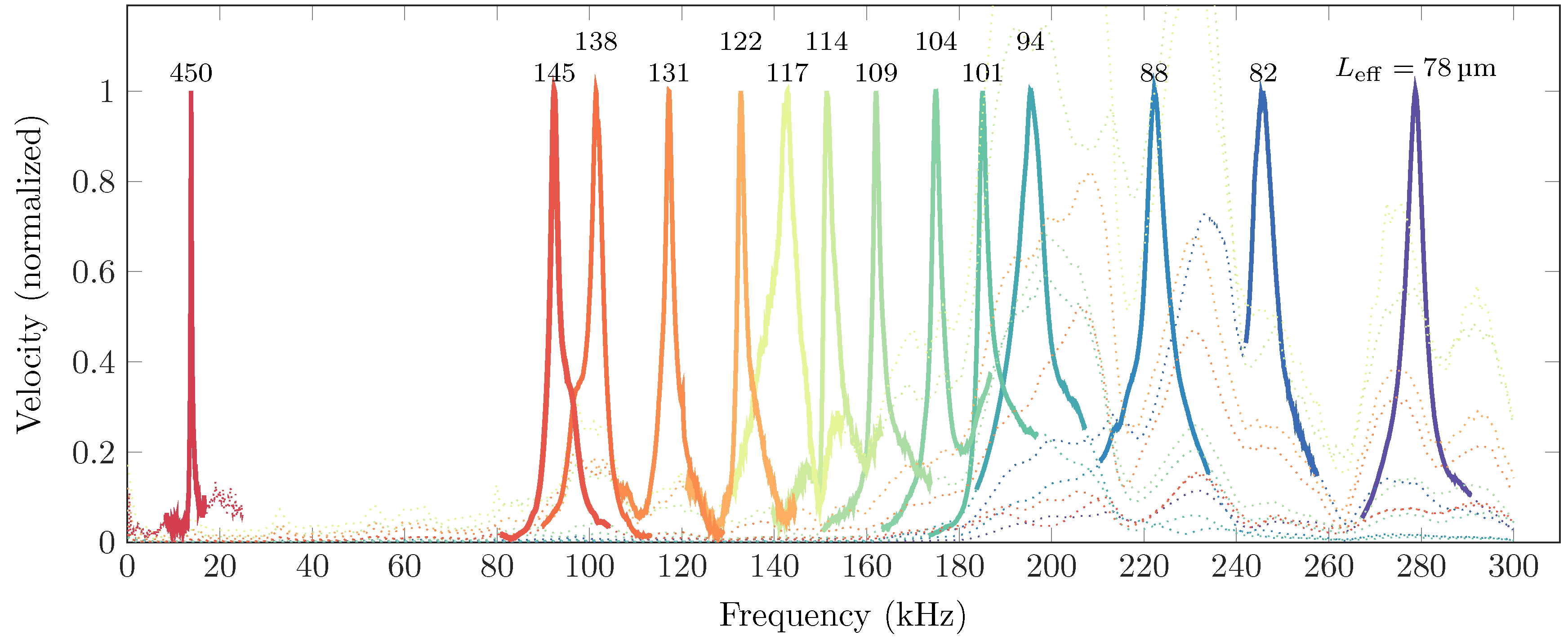
3.2. Experimental Results
4. Discussion
5. Conclusions
Supplementary Files
Supplementary File 1Acknowledgments
Author Contributions
Conflicts of Interest
References
- Binnig, G.; Quate, C.F.; Gerber, C. Atomic Force Microscope. Phys. Rev. Lett. 1986, 56, 930–933. [Google Scholar] [CrossRef] [PubMed]
- Albrecht, T.R.; Quate, C.F. Atomic resolution imaging of a nonconductor by atomic force microscopy. J. Appl. Phys. 1987, 62, 2599–2602. [Google Scholar] [CrossRef]
- Burnham, N.A. Measuring the nanomechanical properties and surface forces of materials using an atomic force microscope. J. Vac. Sci. Technol. A Vac. Surf. Films 1989, 7, 2906–2913. [Google Scholar] [CrossRef]
- Willemsen, O.H.; Snel, M.M.; Cambi, A.; Greve, J.; De Grooth, B.G.; Figdor, C.G. Biomolecular interactions measured by atomic force microscopy. Biophys. J. 2000, 79, 3267–3281. [Google Scholar] [CrossRef]
- Hugel, T.; Seitz, M. The Study of Molecular Interactions by AFM Force Spectroscopy. Macromol. Rapid Commun. 2001, 22, 989–1016. [Google Scholar] [CrossRef]
- Dufrêne, Y.F.; Martínez-Martín, D.; Medalsy, I.; Alsteens, D.; Müller, D.J. Multiparametric imaging of biological systems by force-distance curve-based AFM. Nat. Methods 2013, 10, 847–854. [Google Scholar] [CrossRef] [PubMed]
- Pittenger, B.; Erina, N.; Su, C. Quantitative mechanical property mapping at the nanoscale with PeakForce QNM. Available online: https://www.bruker.com (accessed on 11 April 2016).
- Oesterhelt, F.; Rief, M.; Gaub, H.E. Single molecule force spectroscopy by AFM indicates helical structure of poly(ethylene-glycol) in water. New J. Phys. 1999, 1, 6. [Google Scholar] [CrossRef]
- Kitamura, S.I.; Iwatsuki, M. Observation of 7 × 7 Reconstructed Structure on the Silicon (111) Surface using Ultrahigh Vacuum Noncontact Atomic Force Microscopy. Jpn. J. Appl. Phys. 1995, 34, L145–L148. [Google Scholar] [CrossRef]
- Mueller-Falcke, C.; Song, Y.A.; Kim, S.G. Tunable Stiffness Scanning Microscope Probe. In Proceedings of the Optomechatronic Micro/Nano Components, Devices, and Systems, Philadelphia, PA, USA, 25 October 2004; pp. 31–37.
- Mueller-Falcke, C.; Gouda, S.D.; Kim, S.; Kim, S.S.G. A nanoscanning platform for bio-engineering: An in-plane probe with switchable stiffness. Nanotechnology 2006, 17, S69–S76. [Google Scholar] [CrossRef] [PubMed]
- Vitorino, M.V.; Carpentier, S.; Panzarella, A.; Rodrigues, M.S.; Costa, L. Giant resonance tuning of micro and nanomechanical oscillators. Sci. Rep. 2015, 5. [Google Scholar] [CrossRef] [PubMed]
- Kawai, Y.; Ono, T.; Meyers, E.; Gerber, C.; Esashi, M. Piezoelectric Actuator Integrated Cantilever with Tunable Spring Constant For Atom Probe. In Proceedings of the 19th IEEE International Conference on Micro Electro Mechanical Systems, Istanbul, Turkey, 22–26 January 2006; pp. 778–781.
- Ohler, B. Practical advice on the determination of cantilever spring constants. Available online: http://www.bruker.com (accessed on 11 April 2016).
- Sader, J.E.; Sanelli, J.A.; Adamson, B.D.; Monty, J.P.; Wei, X.; Crawford, S.A.; Friend, J.R.; Marusic, I.; Mulvaney, P.; Bieske, E.J. Spring constant calibration of atomic force microscope cantilevers of arbitrary shape. Rev. Sci. Instrum. 2012, 83. [Google Scholar] [CrossRef] [PubMed]
- Do, C.; Lishchynska, M.; Delaney, K.; Hill, M. Generalized closed-form models for pull-in analysis of micro cantilever beams subjected to partial electrostatic load. Sens. Actuator A Phys. 2012, 185, 109–116. [Google Scholar] [CrossRef]
- Pamidighantam, S.; Puers, R.; Baert, K.; Tilmans, H.A.C. Pull-in voltage analysis of electrostatically actuated beam structures with fixed-fixed and fixed-free end conditions. J. Micromec. Microen. 2002, 12, 458–464. [Google Scholar] [CrossRef]
- Pandey, A.K.; Pratap, R. Effect of flexural modes on squeeze film damping in MEMS cantilever resonators. J. Micromec. Microen. 2007, 17, 2475–2484. [Google Scholar] [CrossRef]
- Muhlstein, C.L.; Brown, S.B.; Ritchie, R.O. High-cycle fatigue of single-crystal silicon thin films. J. Microelectro. Syst. 2001, 10, 593–600. [Google Scholar] [CrossRef]
- Kahn, H.; Ballarini, R.; Heuer, A. Dynamic fatigue of silicon. Curr. Opin. Sol. State Mater. Sci. 2004, 8, 71–76. [Google Scholar] [CrossRef]
- Alsem, D.H.; Pierron, O.N.; Stach, E.A.; Muhlstein, C.L.; Ritchie, R.O. Mechanisms for Fatigue of Micron-Scale Silicon Structural Films. Adv. Eng. Mater. 2007, 9, 15–30. [Google Scholar] [CrossRef]
- Yapu, Z. Stiction and anti-stiction in MEMS and NEMS. Acta Mech. Sin. 2003, 19, 1–10. [Google Scholar] [CrossRef]
- Ziegler, D.; Klaassen, A.; Bahri, D.; Chmielewski, D.; Nievergelt, A.; Mugele, F.; Sader, J.E.; Ashby, P. Encased cantilevers for low-noise force and mass sensing in liquids. In Proceedings of the 2014 IEEE 27th International Conference on Micro Electro Mechanical Systems (MEMS), San Francisco, CA, USA, 26–30 January 2014; pp. 128–131.


© 2016 by the authors; licensee MDPI, Basel, Switzerland. This article is an open access article distributed under the terms and conditions of the Creative Commons by Attribution (CC-BY) license (http://creativecommons.org/licenses/by/4.0/).
Share and Cite
De Laat, M.L.C.; Pérez Garza, H.H.; Ghatkesar, M.K. In situ Stiffness Adjustment of AFM Probes by Two Orders of Magnitude. Sensors 2016, 16, 523. https://doi.org/10.3390/s16040523
De Laat MLC, Pérez Garza HH, Ghatkesar MK. In situ Stiffness Adjustment of AFM Probes by Two Orders of Magnitude. Sensors. 2016; 16(4):523. https://doi.org/10.3390/s16040523
Chicago/Turabian StyleDe Laat, Marcel Lambertus Cornelis, Héctor Hugo Pérez Garza, and Murali Krishna Ghatkesar. 2016. "In situ Stiffness Adjustment of AFM Probes by Two Orders of Magnitude" Sensors 16, no. 4: 523. https://doi.org/10.3390/s16040523