
An Enhanced Energy Balanced Data Transmission Protocol for Underwater Acoustic Sensor Networks

 , ,
, ,
Abstract
:1. Introduction
2. Literature Review
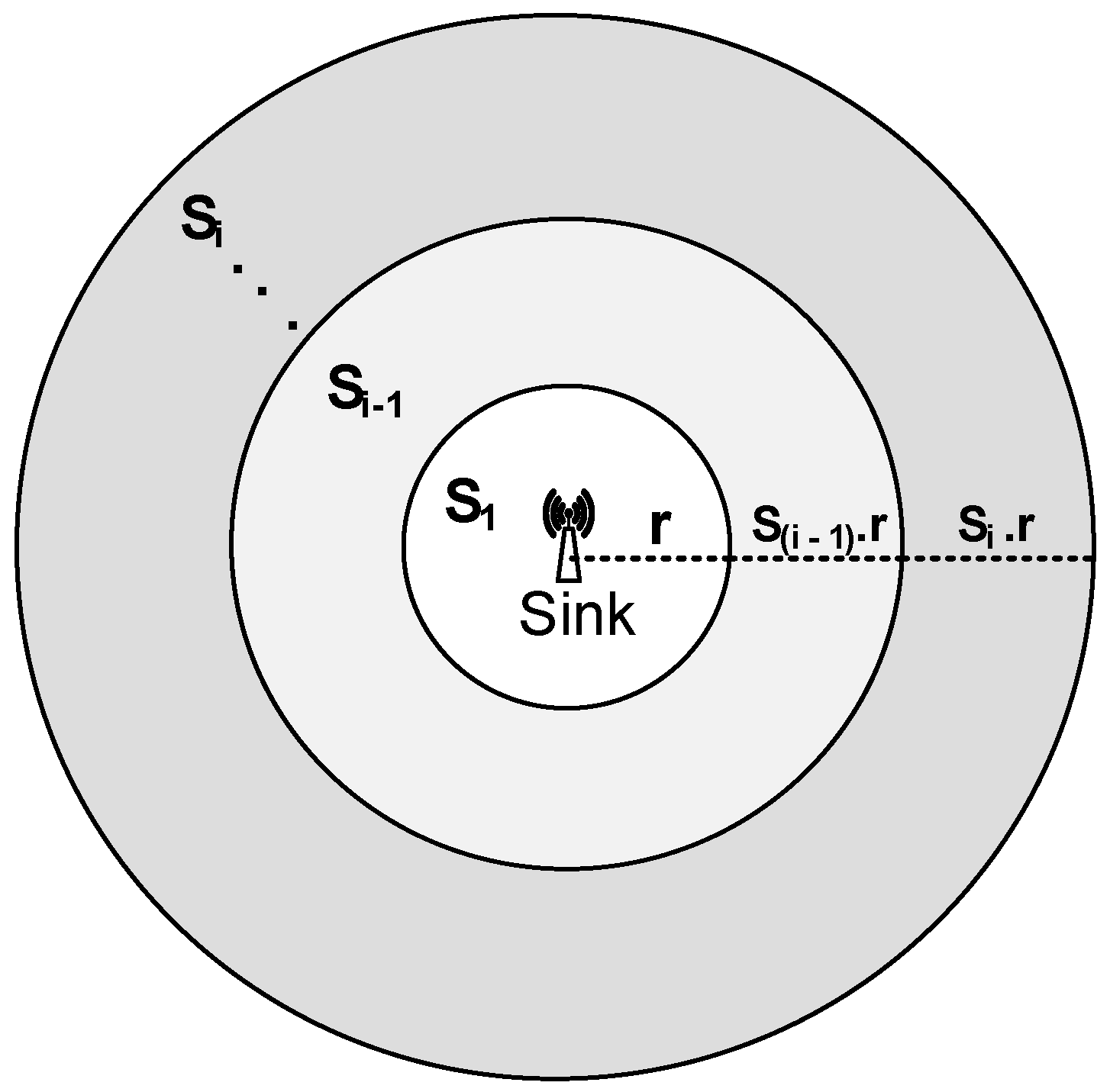
3. Underwater Energy Consumption Model
4. EBET and EEBET: Proposed Techniques
- All sensor nodes are homogeneous with limited battery power and are location-aware using existing positioning method (Received Signal Strength Indicator (RSSI) as location finder [21], and MoteTrack location identification scheme [22]). By location aware we mean that each sensor node knows its location.
- The sensor nodes always have data to send.
- The data reporting mechanism is periodic.
- The static sink resides on the surface of water.
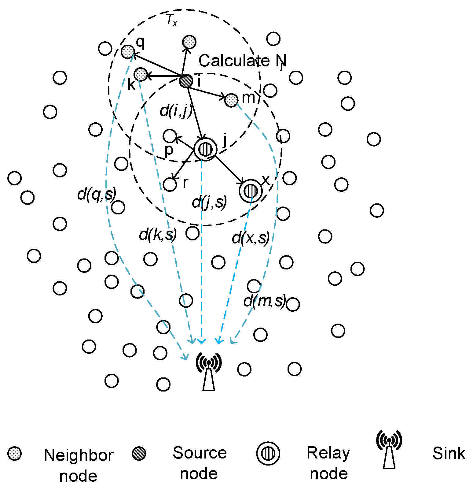
4.1. Protocol Operation
4.1.1. EBET
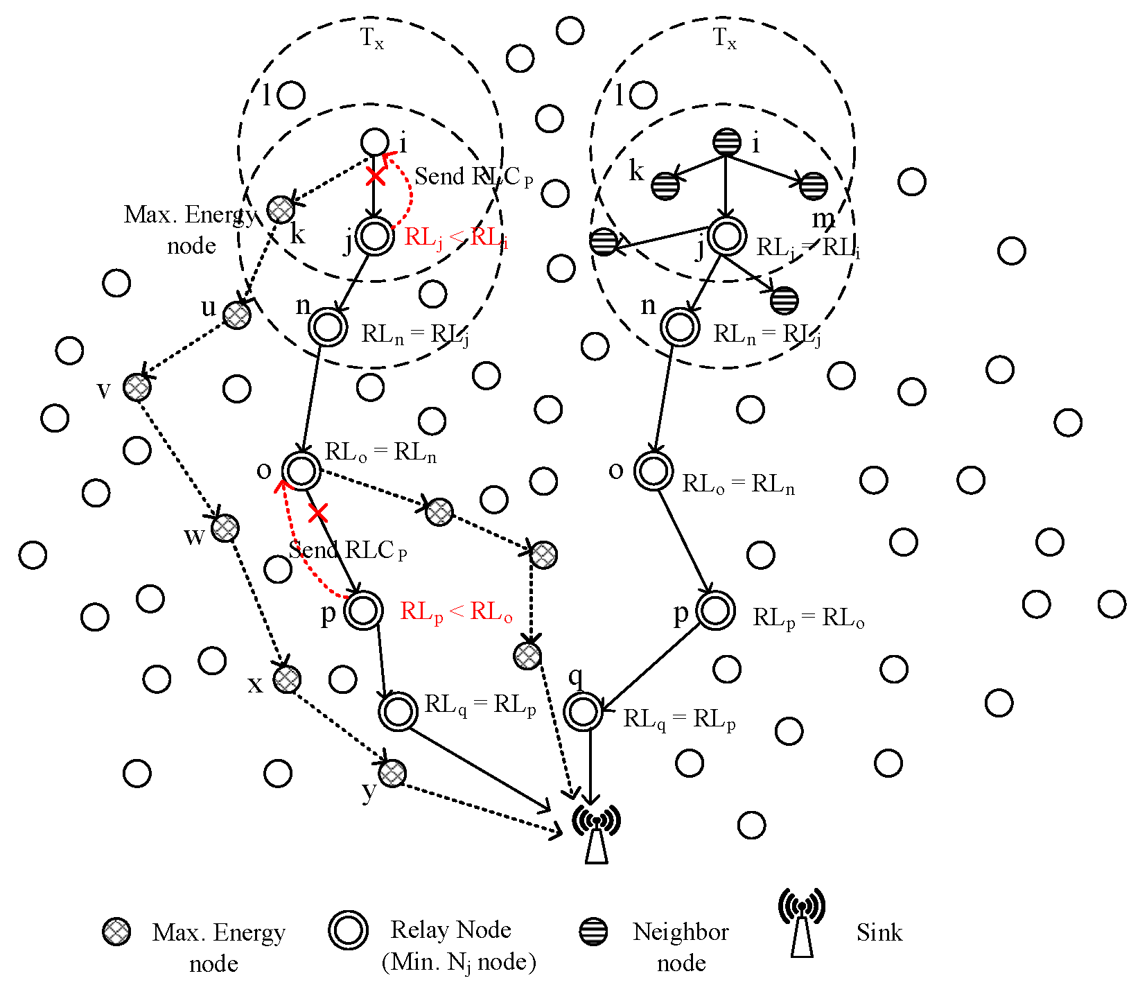
Route Establishment
Data Transmission
| Algorithm 1:: EBET |
|
4.1.2. EEBET
Route Establishment
| Algorithm 2:: Route establishment in EEBET |
|
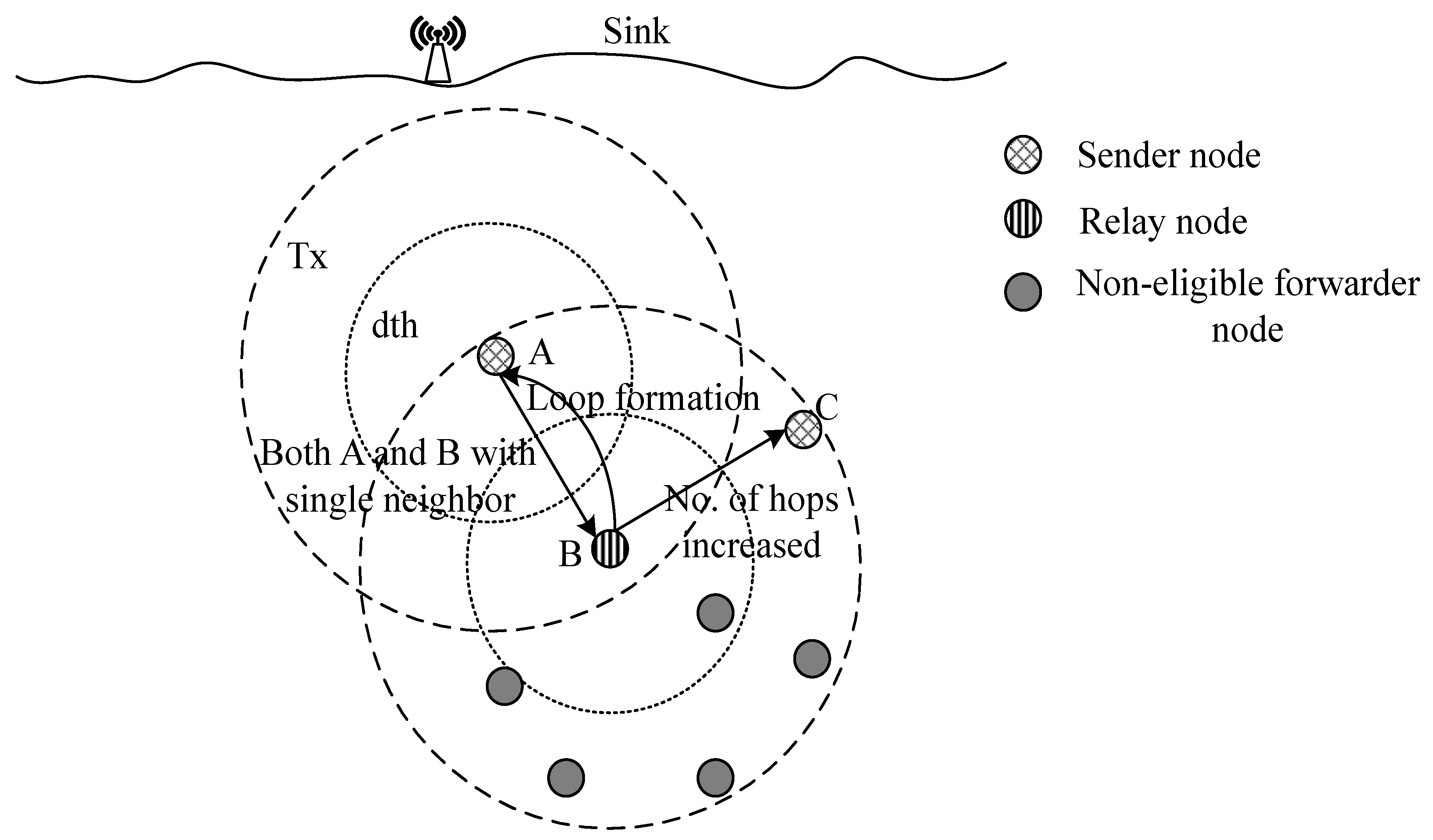
Loop Detection and Elimination
Data Transmission
4.2. Throughput Maximization Model
5. Performance Evaluation
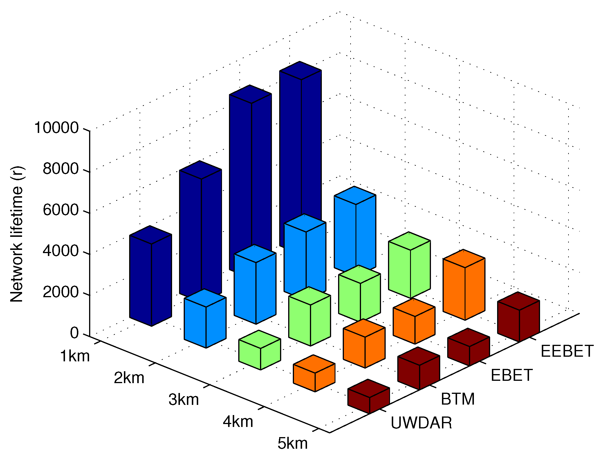
5.1. Impact of Varying Network Radius on Network Lifetime
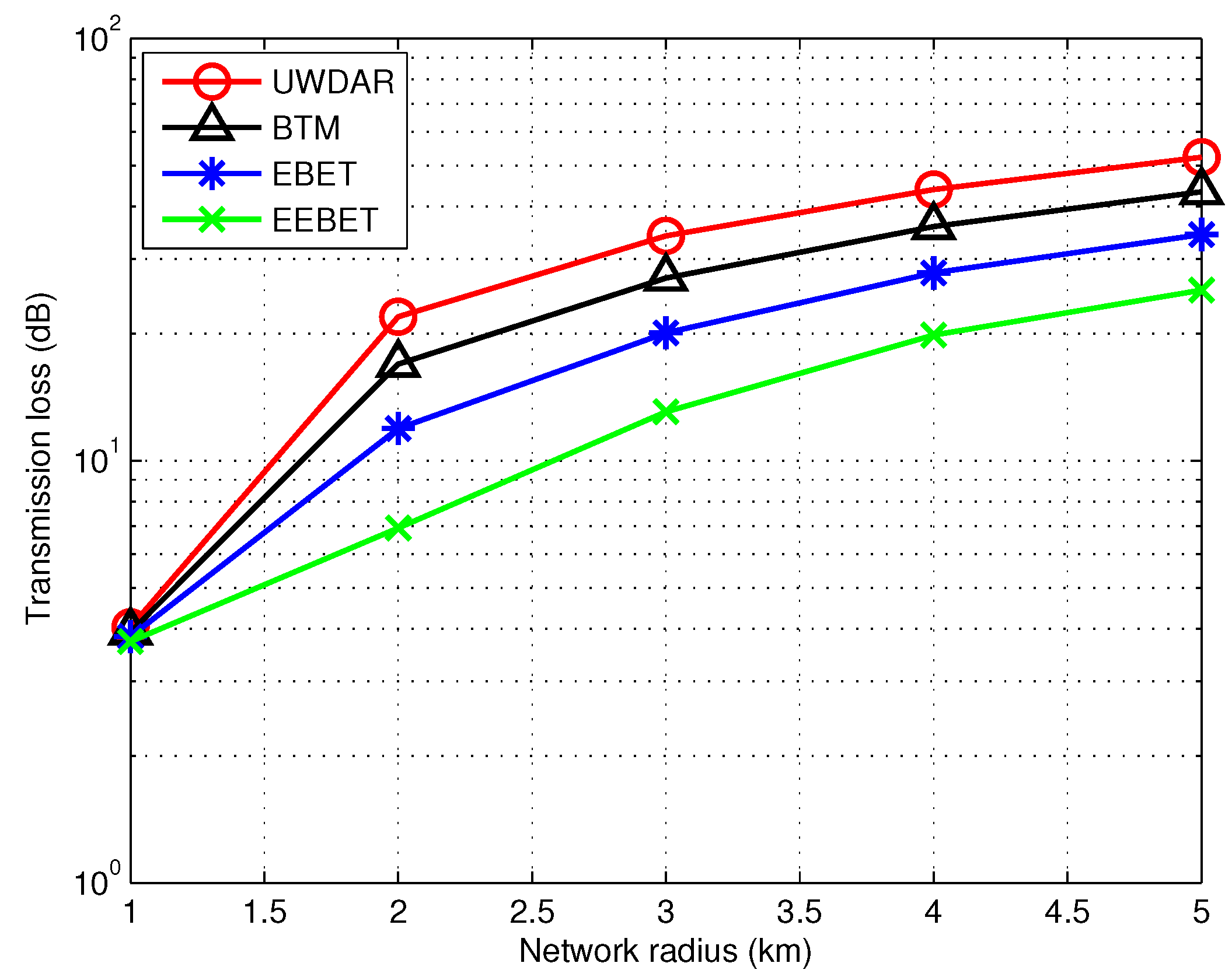
5.2. Impact of Varying Network Radius on Transmission Loss
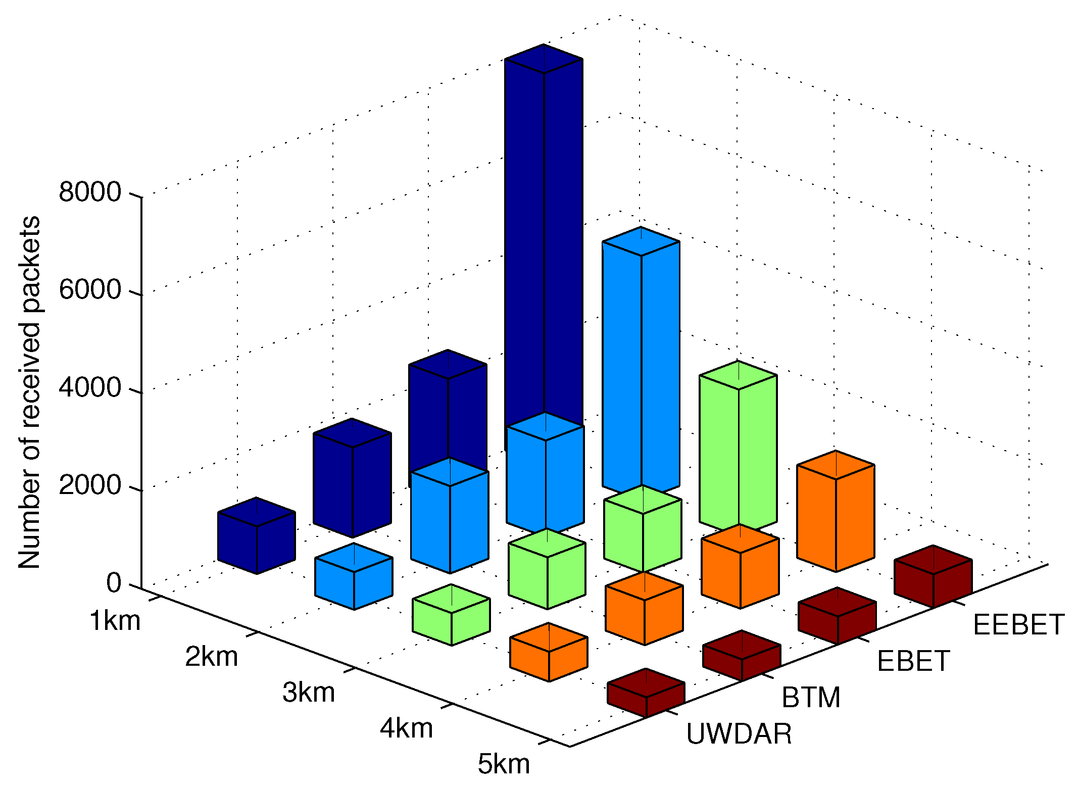
5.3. Impact of Varying Network Radius on Throughput
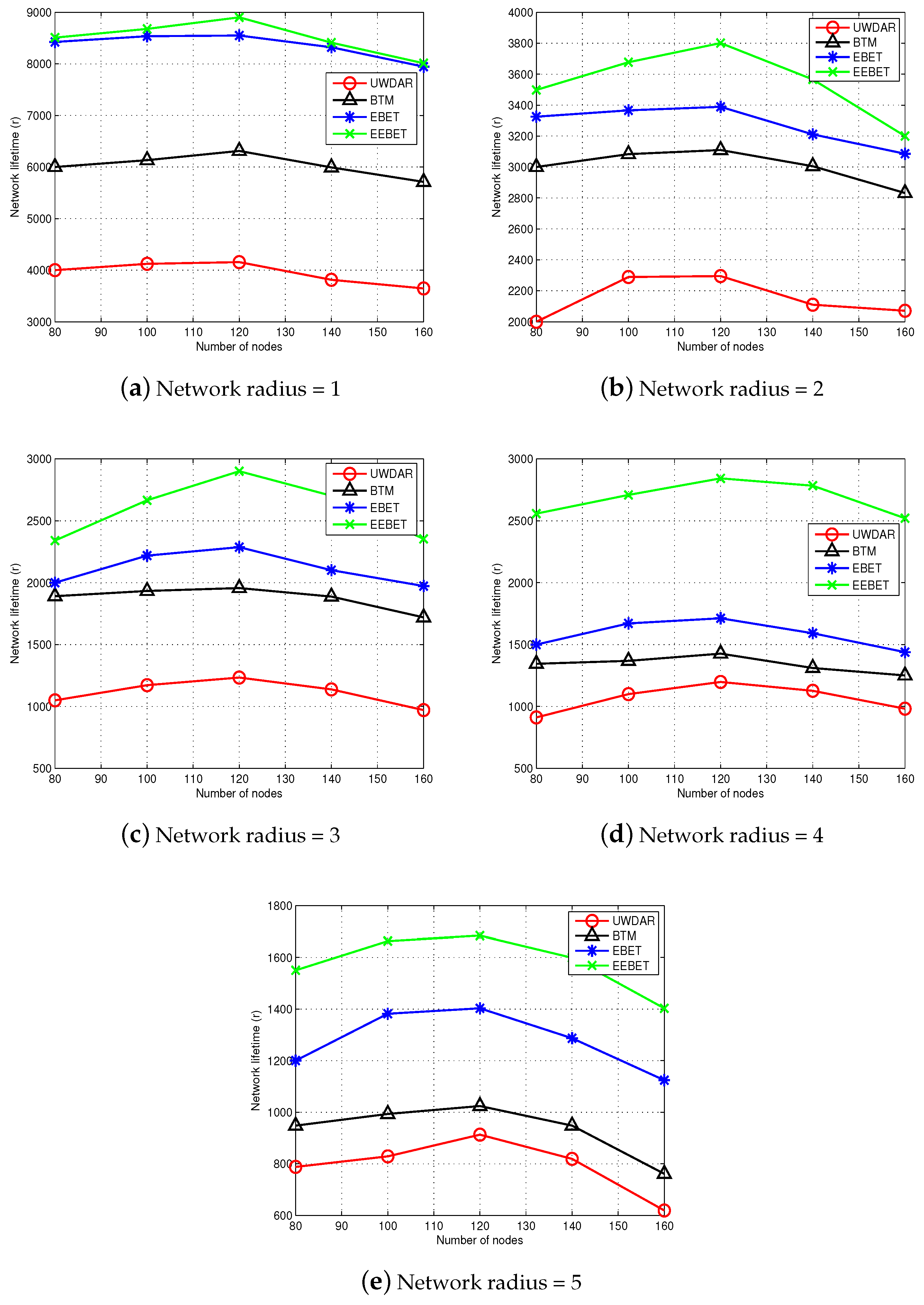
5.4. Impact of Varying Number of Nodes and Varying Network Radius on Network Lifetime
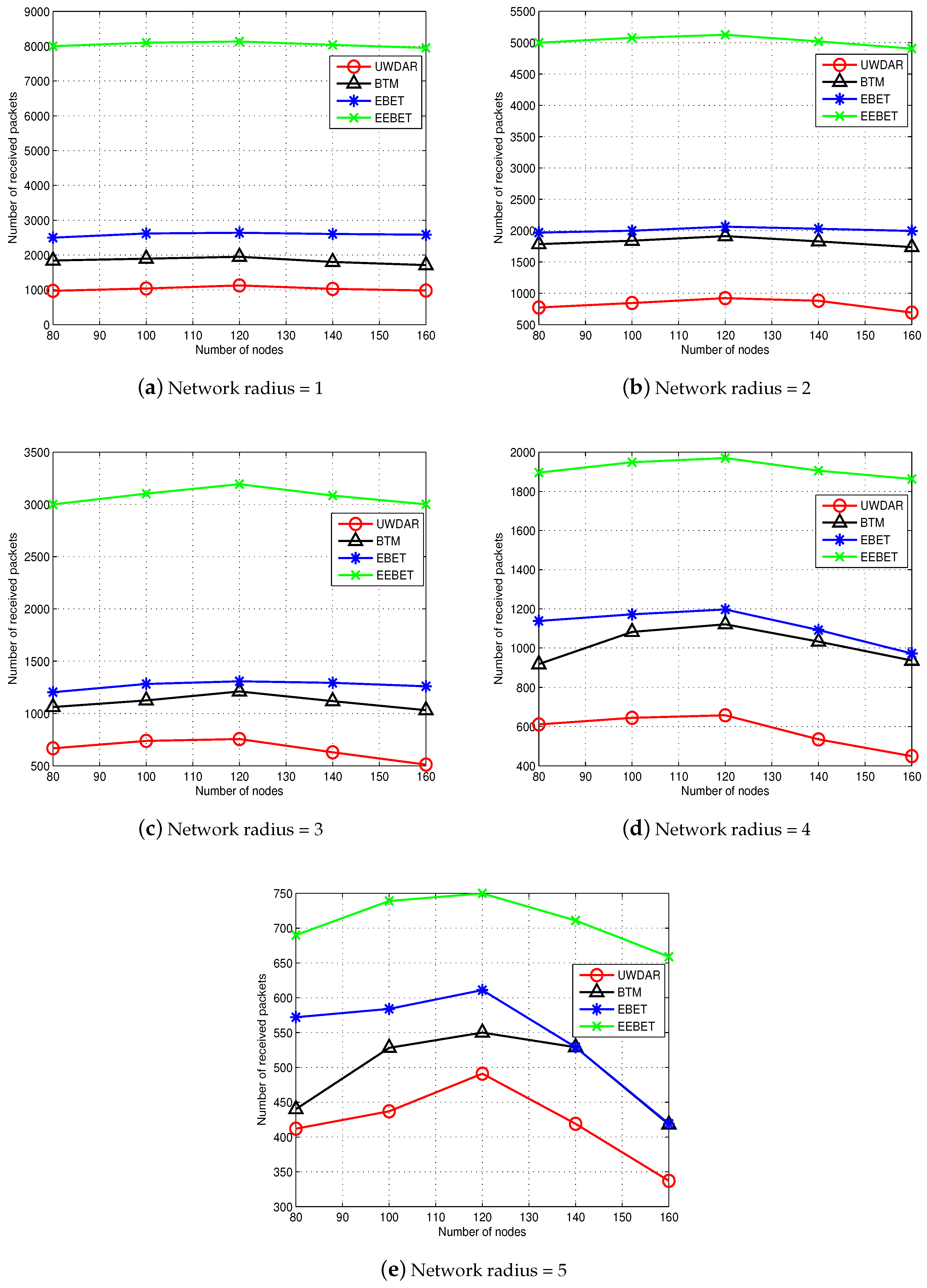
5.5. Impact of Varying Number of Nodes and Varying Network Radius on Throughput
6. Conclusions
Acknowledgments
Author Contributions
Conflicts of Interest
References
- Akyildiz, I.F.; Pompili, D.; Melodia, T. Underwater acoustic sensor networks: Research challenges. Ad Hoc Netw. 2005, 3, 257–279. [Google Scholar] [CrossRef]
- Poncela, J.; Aguayo, M.C.; Otero, P. Wireless underwater communications. Wirel. Pers. Commun. 2012, 64, 547–560. [Google Scholar] [CrossRef]
- Luo, H.; Guo, Z.; Wu, K.; Hong, F.; Feng, Y. Energy balanced strategies for maximizing the lifetime of sparsely deployed underwater acoustic sensor networks. Sensors 2009, 9, 6626–6651. [Google Scholar] [CrossRef] [PubMed]
- Zorzi, M.; Casari, P.; Baldo, N.; Harris, A. Energy-efficient routing schemes for underwater acoustic networks. IEEE J. Sel. Areas Commum. 2008, 26, 1754–1766. [Google Scholar] [CrossRef]
- Wahid, A.; Kim, D. An energy efficient localization-free routing protocol for underwater wireless sensor networks. Int. J. Distrib. Sens. Netw. 2012, 2012, 307246. [Google Scholar] [CrossRef]
- Yan, H.; Shi, Z.J.; Cui, J.H. DBR: Depth-based routing for underwater sensor networks. In NETWORKING 2008 Ad Hoc and Sensor Networks, Wireless Networks, Next Generation Internet; Springer: Berlin, Germany, 2008; pp. 72–86. [Google Scholar]
- Xu, M.; Liu, G.; Wu, H. An energy-efficient routing algorithm for underwater wireless sensor networks inspired by ultrasonic frogs. Int. J. Distrib. Sens. Netw. 2014, 2014, 351520. [Google Scholar]
- Ayaz, M.; Abdullah, A. Hop-by-hop dynamic addressing based (H2-DAB) routing protocol for underwater wireless sensor networks. In Proceedings of the IEEE ICIMT’09 International Conference on Information and Multimedia Technology, Jeju Island, Korea, 16–18 December 2009; pp. 436–441.
- Cao, J.; Dou, J.; Dong, S. Balance Transmission Mechanism in Underwater Acoustic Sensor Networks. Int. J. Distrib. Sens. Netw. 2015, 2015, 429340. [Google Scholar] [CrossRef]
- Dou, J.F.; Zhang, G.X.; Guo, Z.W.; Cao, J.B. PAS: Probability and sub-optimal distance-based lifetime prolonging strategy for underwater acoustic sensor networks. Wirel. Commun. Mob. Comput. 2008, 8, 1061–1073. [Google Scholar] [CrossRef]
- Li, Z.; Yao, N.; Gao, Q. Relative Distance Based Forwarding Protocol for Underwater Wireless Networks. Int. J. Distrib. Sens. Netw. 2014, 2014, 173089. [Google Scholar] [CrossRef]
- Harris, A.F.; Stojanovic, M.; Zorzi, M. When underwater acoustic nodes should sleep with one eye open: Idle-time power management in underwater sensor networks. In Proceedings of the 1st ACM International Workshop on Underwater Networks, Los Angeles, CA, USA, 25 September 2006; pp. 105–108.
- Syed, A.; Ye, W.; Heidemann, J. T-Lohi: A new class of MAC protocols for underwater acoustic sensor networks. In Proceedings of the IEEE 27th Conference on Computer Communications (INFOCOM 2008), Phoenix, AZ, USA, 13–18 April 2008.
- Shah, M.; Javaid, N.; Tariq, S.; Imran, M.; Alnuem, M. A Balanced Energy Consumption Protocol for Underwater ASNs. In Proceedings of the 18th IEEE International Conference on Network-Based Information Systems (NBiS-2015), Taipei, Taiwan, 2–4 September 2015.
- Pompili, D.; Melodia, T.; Akyildiz, I.F. Routing algorithms for delay-insensitive and delay-sensitive applications in underwater sensor networks. In Proceedings of the 12th Annual International Conference on Mobile Computing and Networking, Los Angeles, CA, USA, 24–29 September 2006; pp. 298–309.
- Wahid, A.; Lee, S.; Kim, D. An energy-efficient routing protocol for UWSNs using physical distance and residual energy. In Proceedings of the 2011 IEEE-Spain OCEANS, Santander, Spain, 6–9 June 2011; pp. 1–6.
- Mahmood, S.; Nasir, H.; Tariq, S.; Ashraf, H.; Pervaiz, M.; Khan, Z.A.; Javaid, N. Forwarding Nodes Constraint based DBR (CDBR) and EEDBR (CEEDBR) in Underwater WSNs. Procedia Comput. Sci. 2014, 34, 228–235. [Google Scholar] [CrossRef]
- Doyle, L. A multi-hop ARQ protocol for underwater acoustic networks. In Proceedings of the OCEANS 2007—Europe, Aberdeen, UK, 18–21 June 2007.
- Bi, Y.; Li, N.; Sun, L. DAR: An energy-balanced data-gathering scheme for wireless sensor networks. Comput. Commun. 2007, 30, 2812–2825. [Google Scholar] [CrossRef]
- Stojanovic, M. On the relationship between capacity and distance in an underwater acoustic communication channel. ACM SIGMOBILE Mob. Comput. Commun. Rev. 2007, 11, 34–43. [Google Scholar] [CrossRef]
- Kwak, K.M.; Kim, J. Development of 3-dimensional sensor nodes using electro-magnetic waves for underwater localization. J. Inst. Control Robot. Syst. 2013, 19, 107–112. [Google Scholar] [CrossRef]
- Lorincz, K.; Welsh, M. Motetrack: A robust, decentralized approach to RF-based location tracking. In Location- and Context-Awareness; Springer: Berlin, Germany, 2005; pp. 63–82. [Google Scholar]
- Imran, M.; Alnuem, M.A.; Fayed, M.S.; Alamri, A. Localized Algorithm for Segregation of Critical/Non-Critical Nodes in Mobile Ad Hoc and Sensor Networks. Procedia Comput. Sci. 2013, 19, 1167–1172. [Google Scholar] [CrossRef]
- Ahmad, A.; Javaid, N.; Khan, Z.A.; Qasim, U.; Alghamdi, T.A. (ACH)2: Routing Scheme to Maximize Lifetime and Throughput of Wireless Sensor Networks. IEE Sens. J. 2014, 14, 3516–3532. [Google Scholar] [CrossRef]


| Technique | Features | Domain | Flaws/Deficiencies | Achievements |
|---|---|---|---|---|
| BTM [9] | Balanced energy consumption, Energy efficient | UASNs, 2D underwater terrain monitoring | High energy consumption while transmitting at long distance, Formation of transmission loops | Network lifetime, Balanced energy consumption |
| EBH and DIB [3] | Energy balancing, Applicable for both shallow and deep water | 2D UASNs, Moored monitoring systems, Oceanographic data collection | Inefficient for other than linear networks, Designed only for sparse network | Network lifetime, Balanced energy consumption |
| H2-DAB [8] | Energy efficient, Dimensional location information is not required | UASNs, Critical underwater monitoring missions | Imbalanced energy consumption, Nearer to sink nodes deplete energy earlier, High end-to-end delay | High data delivery ratio, Network lifetime |
| RAD [15] | Energy efficient, Acoustic channel utilization efficiency, Introduces forward error correction | 3D UASNs, Geographical routing for delay-sensitive and delay-insensitive applications | Imbalanced energy consumption, Increase in packet size increases packet error rate, Solution for concave node (void region) is not provided | Low packet error rate, Minimized energy consumption, Low end-to-end delay |
| ERP2R [16] | Energy efficient, Physical distance and residual energy based routing | 3D UASNs, Underwater monitoring, Location-based routing | Imbalanced energy consumption with the growth of node mobility, Longer routing paths, Duplicate packets transmission | Network lifetime, Minimized end-to-end delay and energy consumption |
| RDBF [11] | Energy efficient, Minimum hop counts involved, No exchange of control messages | 3D UASNs, Underwater monitoring and target tracking applications, Location-based routing | Do not restrict forwarding area for packets, All nodes with same distance with the sink send same packets at the same time | Network lifetime, High packet delivery ratio, Low end-to-end delay |
| DBR [6] | Full dimensional location information of sensor nodes is not required | UASNs, 3D underwater monitoring, Depth based routing, Handles dynamic networks | High energy consumption, Imbalanced energy consumption, Data redundancy, Inefficient for sparse and highly dense networks | Network lifetime, High data delivery ratio, Low end-to-end delay |
| EEDBR [5] | Energy efficient, No dimensional location information required, Controlled flooding | UASNs, 3D underwater monitoring and surveillance applications | Imbalanced energy consumption, High energy consumption in dense networks, Low packet delivery ratio, High packet drop rate | Network lifetime, Minimum energy consumption, End-to-end delay |
| UFCA [7] | Energy efficient, No periodic flooding messages required, Uses Gravity function for data routing | 3D-UASNs, Underwater surveillance and monitoring applications, Distributed routing mechanism | Imbalanced energy consumption, Resistant to node mobility, Temporary loss of connectivity, Routing information may not be updated, High end-to-end delay | High packet delivery ratio, Minimized energy consumption, Scalability |
| CDBR/CEEDBR [17] | Energy efficient, Limited forwarder nodes, Depth-dependent | 3D-UASNs, Underwater monitoring and surveillance | Imbalanced energy consumption, High packet drop and end-to-end delay, Static network topology | Network lifetime, Minimized energy consumption |
| (km) | R (km) |
|---|---|
| 0.15 | 1 |
| 0.225 | 1.5 |
| 0.3 | 2 |
| 0.375 | 2.5 |
| 0.45 | 3 |
| 0.525 | 3.5 |
| 0.6 | 4 |
| 0.675 | 4.5 |
| 0.75 | 5 |
| Parameter | Value |
|---|---|
| R | 1–5 km |
| N | 80 |
| 300 J | |
| f | 20 kHz |
| 0.2 × J/bit |
© 2016 by the authors; licensee MDPI, Basel, Switzerland. This article is an open access article distributed under the terms and conditions of the Creative Commons by Attribution (CC-BY) license (http://creativecommons.org/licenses/by/4.0/).
Share and Cite
Javaid, N.; Shah, M.; Ahmad, A.; Imran, M.; Khan, M.I.; Vasilakos, A.V. An Enhanced Energy Balanced Data Transmission Protocol for Underwater Acoustic Sensor Networks. Sensors 2016, 16, 487. https://doi.org/10.3390/s16040487
Javaid N, Shah M, Ahmad A, Imran M, Khan MI, Vasilakos AV. An Enhanced Energy Balanced Data Transmission Protocol for Underwater Acoustic Sensor Networks. Sensors. 2016; 16(4):487. https://doi.org/10.3390/s16040487
Chicago/Turabian StyleJavaid, Nadeem, Mehreen Shah, Ashfaq Ahmad, Muhammad Imran, Majid Iqbal Khan, and Athanasios V. Vasilakos. 2016. "An Enhanced Energy Balanced Data Transmission Protocol for Underwater Acoustic Sensor Networks" Sensors 16, no. 4: 487. https://doi.org/10.3390/s16040487