1. Introduction
An electronic nose (E-nose) is a device composed of a gas sensor array and an artificial intelligence algorithm. They are effective in dealing with odor analysis problems [
1,
2,
3], and have been introduced to many fields such as environmental monitoring [
4,
5], food engineering [
6,
7,
8], disease diagnosis [
9,
10,
11,
12], explosives detection [
13] and spaceflight applications [
14].
Most of the time during a person’s life is spent indoors, so it is significant to monitor changes in indoor gas composition, and it is necessary for people’s health to detect the indoor pollutant gases as early as possible. Consequently, there has been a resurgence of interest in developing measurement techniques for air quality monitoring. Our previous work has proved that E-noses are an effective way to classify indoor pollutant gases [
15,
16].
To study the patterns of different indoor pollutant gases, many sampling experiments must be done on each gas. In the past, we only processed labeled data by feature extraction methods [
17,
18], however, in actual experiments, the numbers of collected unlabeled samples are often far greater than that of the labeled samples, and they are easier to obtain while the cost of getting the labeled samples is usually higher than for unlabeled ones. On the other hand, in the sampling experiments, there can be unexpected mistakes such as the paper label identifying the target gas which is pasted on the gas bag is lost, the label information is not written down because of a fault of operators which will lead to the loss of the sample label, which all causes a certain amount of waste of the number of experimental samples. Although the classification accuracy of E-noses trained by labeled samples is usually higher than that of devices trained with unlabeled samples, it is often difficult to obtain sufficient labeled samples. What’s more, there is a lot of hidden information in the unlabeled samples. Therefore, researchers have put forward algorithms to train E-noses with labeled sample as well as make full use of available unlabeled samples.
To make full use of unlabeled samples, researchers have proposed various methods in the past. These methods can be divided into three categories: (1)
Active learning: this is a learning paradigm that requires users’ (or some other information source) interaction to provide the responses of new data points [
19,
20]; (2)
Transfer learning: these are methods that focus on applying the knowledge learned from related, but different tasks to solve the target task [
21,
22,
23]. They usually require sufficient labeled data to acquire accurate knowledge; (3)
Semi-supervised learning (SSL): these techniques aim at learning an inductive rule or try to accurately determine the label of the data from a small amount of labeled data with the help of a large amount of unlabeled data [
24,
25,
26]. For its ability to solve classification and regression problems by learning from a set of labeled data and unlabeled samples, this last approach has been widely adopted in various application domains such as hand-writing recognition [
27] and bioinformatics [
28].
In 2012, De Vi
et al. applied a semi-supervised boosting algorithm to an artificial olfaction classification problem and proposed a novel SSL-based algorithm for an air pollution monitoring data set [
29]. This work can be thought as the first time of SSL was adopted in E-nose research. Liu
et al. also proposed a domain adaptation technique which can be seen as a SSL technique in 2014, and this technique was adopted to eliminate the E-nose signal drift [
30].
Tri-training is a SSL techniques [
31] which doesn’t require sufficient and redundant samples, nor does it require the use of different supervised learning algorithms. Inspired by tri-training, a novel multi-class SSL technique which is called as M-training is proposed in this paper to train E-noses with both labeled samples and unlabeled samples. The rest of this paper is organized as follows:
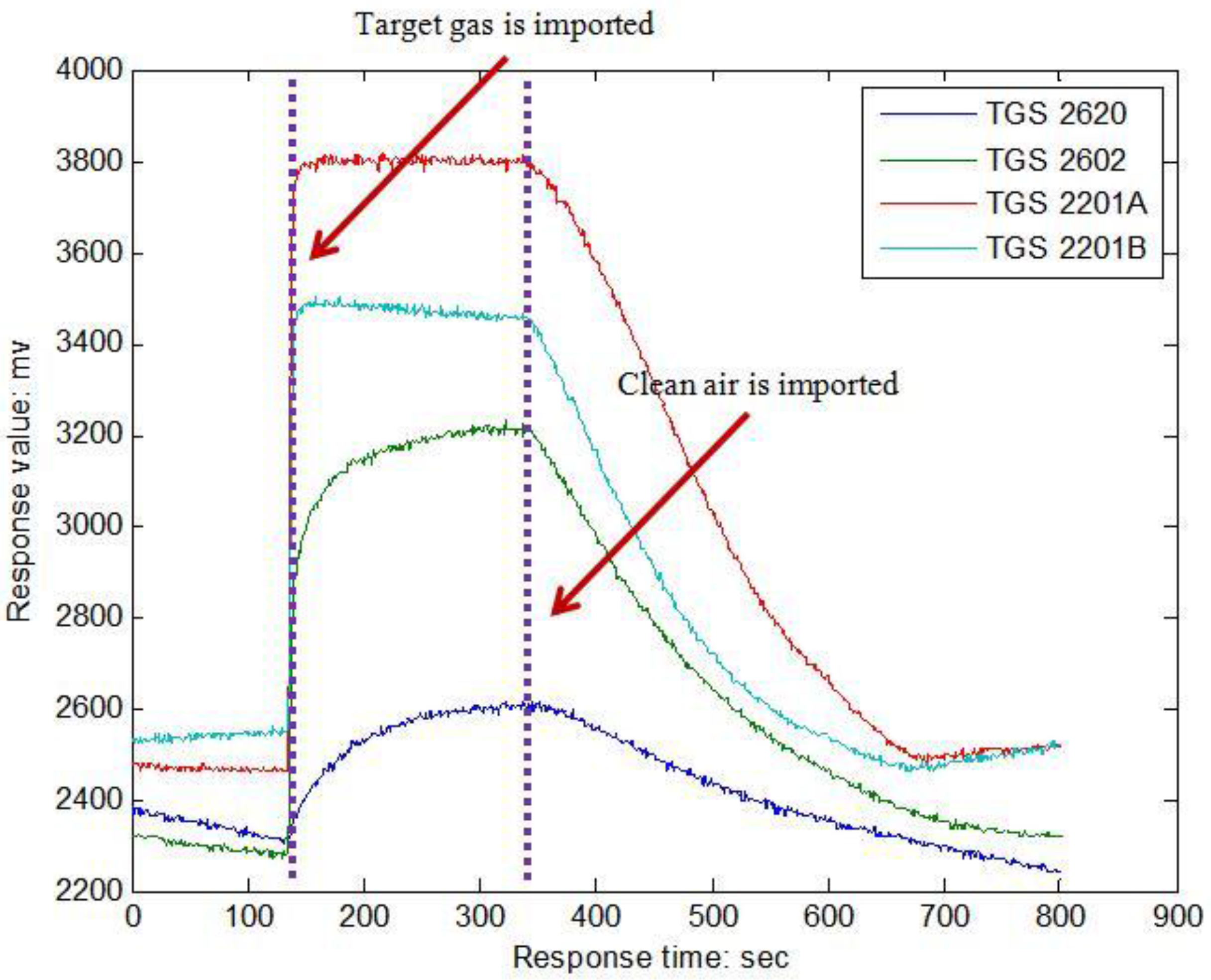
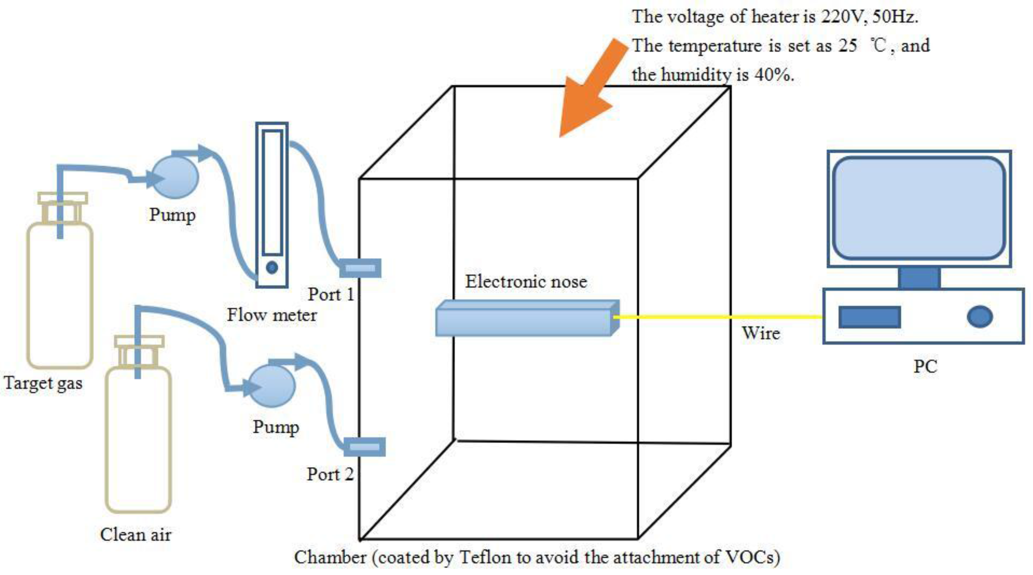
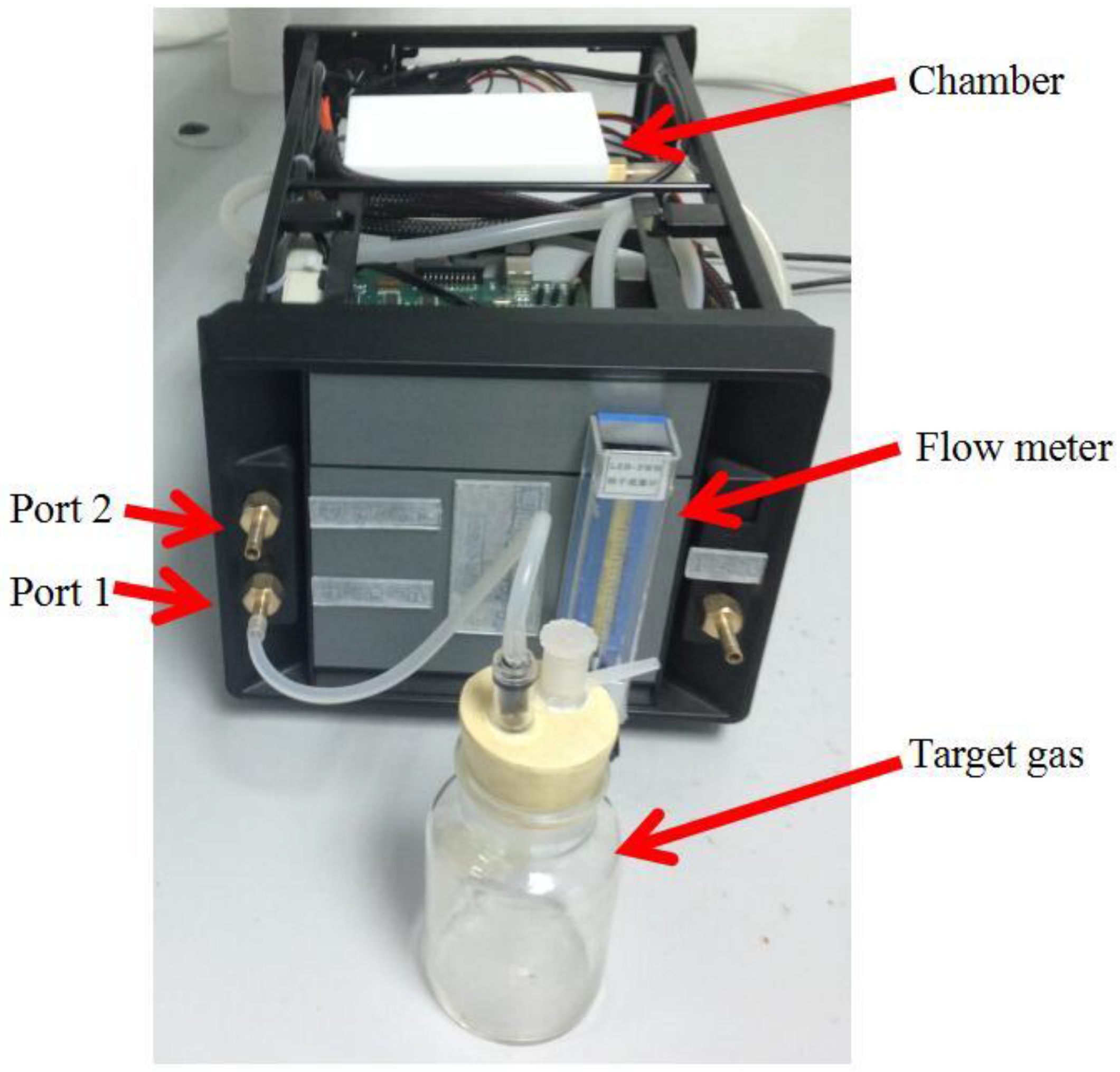
Section 2 introduces the E-nose system and gas sampling experiments of this paper;
Section 3 presents the theory of M-training technique;
Section 4 describes the results of M-training when it is used to train the E-nose classifier for predicting the classes of target pollutant gases. Finally, we draw the conclusions of this paper in
Section 5.
3. M-Training Technique
As a SSL technique, M-training retains the advantages of tri-training, while, more base classifiers can be employed by M-training which gives it have more opportunity to learn and obtain knowledge from the unlabeled samples.
Let L denote the labeled sample set with size |L| and U denote the unlabeled sample set with size |U|. There are M base classifiers in M-training, denoted as , where M is a positive integer, and M ≥ 3. M-training will degenerate to tri-training when M is set as 3. These base classifiers have been trained by the samples from set L. During the learning process of M-training, each ci will be the main classifier in a cycle, meanwhile, the other classifiers are employed to predict the class label of samples from U (for simply, these classifiers are denoted as ). Whether one sample of set U will be used to train the main classifier ci combining with set L depends on the degree of agreements (made by classifiers of Ci) on its labeling, namely, if the classifiers of Ci voting for a particular label exceeds a threshold , then this sample along with its label (predicted by Ci) will be used to refine the main classifier ci combining with set L.
In the M-training technique, the misclassification of unlabeled samples is unavoidable, so ci will receive noisy samples from time to time. Fortunately, even in the worst case, the increase in classification noise rate can be compensated if the amount of newly labeled samples is sufficient and meet certain conditions. These conditions are introduced as follows:
Inspired by Goldman
et al. [
32], the finding of Angluin
et al. [
33] is employed. Suppose there is a training data set containing
m samples, and the noise rate is
η, then the worst case error rate
of the classifier satisfies Equation (1):
where
is a constant, then Equation (1) can be reformulated as Equation (2):
In each round of M-training, Ci chooses samples in U to label for ci. The amount and the concrete unlabeled samples chosen to label would be different in different rounds because ci is refined in each round. We denote by Li(t) and Li(t – 1) the set of samples which are labeled by Ci for ci in round t and round t – 1, respectively. Then the training data set for ci in round t and t – 1 can be expressed as and , respectively. It should be noted that Li(t – 1) will be regarded as the unlabeled data and put back to U during round t.
Let
ηL denote the classification noise rate of
L, so the number of mislabeled samples in
L is
ηL|
L|. Let
ei(
t) be the upper bound of the classification error rate of
Ci in round
t. Assuming there are
n samples which are labeled by
Ci, and among these samples,
Ci makes the correct classification on
n’ samples, then
ei(
t) can be estimated as (
n – n’)/
n. Thus, the number of mislabeled samples in
Li(
t) is
. Therefore the classification noise rate in round
t is:
Thus, Equation (2) can be computed as:
Similarly,
can be computed by Equation (5):
If we want
, then
according to Equation (2), which means that the performance of
ci can be improved through utilizing
Li(
t) in its training. This condition can be expressed as Equation (6):
Considering that
can be very small and assuming
, then the first part on the left hand of Equation (6) is bigger than its correspondence on the right hand if
, and the second part on the left hand is bigger than its correspondence on the right hand if
. These restrictions can be expressed into the condition shown in Equation (7), and this condition is employed by M-training to decide whether one unlabeled sample could be labeled for
ci:
Note that
may still be less than
even if
and
due to the fact that
may be much bigger than
. When this happens, a sub-sampling method presented in paper [
31] is employed, and the detail operation is shown as follows: in some cases
could be randomly sub-sampled such that
. Given
,
and
, let integer
denote the size of
after sub-sampling, then if Equation (8) holds,
will be satisfied:
where
should satisfy Equation (9) such that the size of
after sub-sampling is still bigger than
:
It is noteworthy that the initial base classifiers should be diverse because if all classifiers are identical, then for any ci, the unlabeled samples labeled by classifier of Ci will be the same as ci. To achieve the diversity of the base classifiers, each base classifier just randomly employ 75% of set L as its initial training data set, and the training data set of each classifier will be different via this way.
Finally, the process of M-training can be listed as follows:
Step (a): Prepare data set L, U and the test data set for E-nose; set the value of M and θ.
Step (b): Train each base classifier ci of M-training with the initial training data set Li generated randomly from set L.
Step (c): Gain the initial classification accuracy of set L and the initial classification accuracy of the test data set. Simple voting technique is employed to determine the predict label of one sample, and all base classifiers of M-training are used to predict the gas during this step.
Step (d): Repeat the following process until none of , changes:
(d.1) Compute , as it has been introduced that , where means the samples of set U labeled by in round t, and is the samples of set U labeled correctly by Ci. However it is impossible to estimate the classification error on the unlabeled samples, and only set L is available, heuristically based on the assumption that the unlabeled samples hold the same distribution as that held by the samples of set U;
(d.2) If , any sample of set U will be used to generate set if the agreement of labeling this sample made by classifiers in exceeds ;
(d.3) If , then there will be two cases: case (1) , classifier will be refined by , and , if ; case (2) , then samples of will be removed, where is computed by Equation (8), then will be refined.
Step (e): Obtain the final classification accuracy of set L and the final classification accuracy of the test data set, and the computation process is the same as step (c).
4. Results and Discussion
The first task of this section is to decide which classifier can be used as the base classifier of M-training. Partial least square discriminant analysis (PLS-DA) [
34], radial basis function neural network (RBFNN) [
35] and support vector machine (SVM) [
36,
37] are considered in this paper. The leave-one-out technique (LOO) is used to train and test the three classifiers. Classification accuracy of the training data set and test data set is set to evaluate the performance of the three classifiers. To make sure every classifier achieves its best working state, an enhanced quantum-behaved particle swarm optimization (EQPSO) [
38] is used to optimize the parameters. Each program is repeated for 10 times among which the best result will be the final result of each classifier. The results are shown in
Table 4.
It is clear that the classification accuracy of SVM has the highest accuracy rate of all classifiers, so SVM is selected as the base classifier for M-training. The value of parameters in these three methods are set as follows: the number of latent variables of PLS-DA is 5; the goal MSE and the spread factor of RBFNN are 0.4329 and 0.0176, respectively; RBF function is employed as the kernel of SVM and its value is 0.2749, while the value of the penalty factor of SVM is 0.4848.
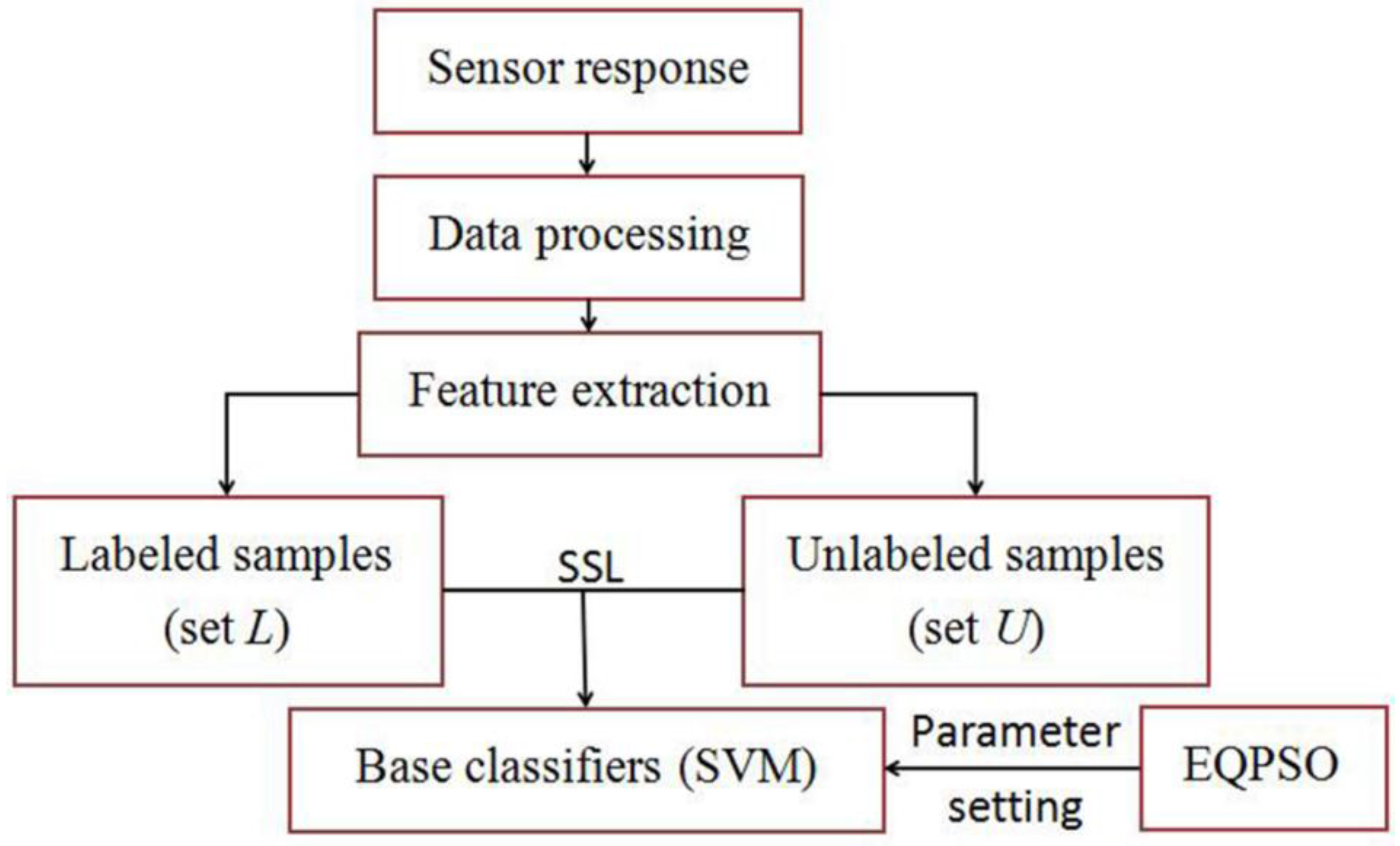
Then tri-training and M-training with a different number of base classifiers are employed to refine the classifier of our E-nose. The flow chart of SSL process is shown as
Figure 4. Half of the training data set is defined as data set
L which is used to train the base classifiers, and the rest of the training data set are set as set
U which is used to refine the base classifiers, namely, the unlabeled rate is 50%. The threshold
θ of M-training is set as
. The classification results of both methods are shown in
Table 5.
As one can see, the M-training results are better than those of tri-training. The reason is analyzed as follows: suppose there is a point in set U (whose real label is 1). There are three classifiers in tri-training, this point will not be considered to train classifier 1 if classifier 2 predicts the label of this point is 1 and classifier 3 predicts its label is 2. Meanwhile, suppose there are four classifiers in M-training, and classifier 2 and classifier 3 make the same classification as the corresponding classifier in tri-training, then this point will be considered to refine classifier 1 if classifier 4 predicts the label is 1, so M-training has more opportunity to refine its base classifiers, and this ensures that the E-nose has more opportunity to learn knowledge from the unlabeled points.
It can also be found from
Table 5 that the classification results of M-training with four base classifiers are the same as M-training with five or six base classifiers. Although more base classifiers means more opportunities to learn from the unlabeled samples, the knowledge provided by unlabeled samples is limited when the set of unlabeled samples is determined. One can enlarge the size of unlabeled set to make the classification accuracy of E-nose more ideal.
The highest classification accuracy in
Table 5 is 96.97% obtained by M-training when four base classifiers are trained by
L and refined by
U (the unlabeled rate is 50%). To study how much potential knowledge has been recovered from the unlabeled samples, we set another training process during which there are four classifiers (SVM) and they are trained by the whole training data set (
L +
U). The final classifier result is decided by simple voting, and its corresponding classification accuracy of the test data set is 98.48%. We can find this result is much higher than 74.24% (obtained when the four base classifiers of M-training are just trained by set
L) and is just little higher than 96.97%. This comparison indicates that much useful knowledge has been found by the E-nose in the unlabeled data with the help of M-training.
Finally, the performance of M-training (four base classifiers) with different unlabeled rates (75%, 50% and 25%) of the training data set is researched. An introduction about the amount of samples in each data set is given in
Table 6.
Table 7,
Table 8 and
Table 9 list the results of the M-training technique with different unlabeled sample rates, and it is clear that the unlabeled samples can improve the classification accuracy of the test data set no matter what the unlabeled rate is.
Table 10 lists the amount of samples in each
ci with different unlabeled rate, and one can find that more samples are used to train the base classifier when M-training is adopted to train and refine E-nose.
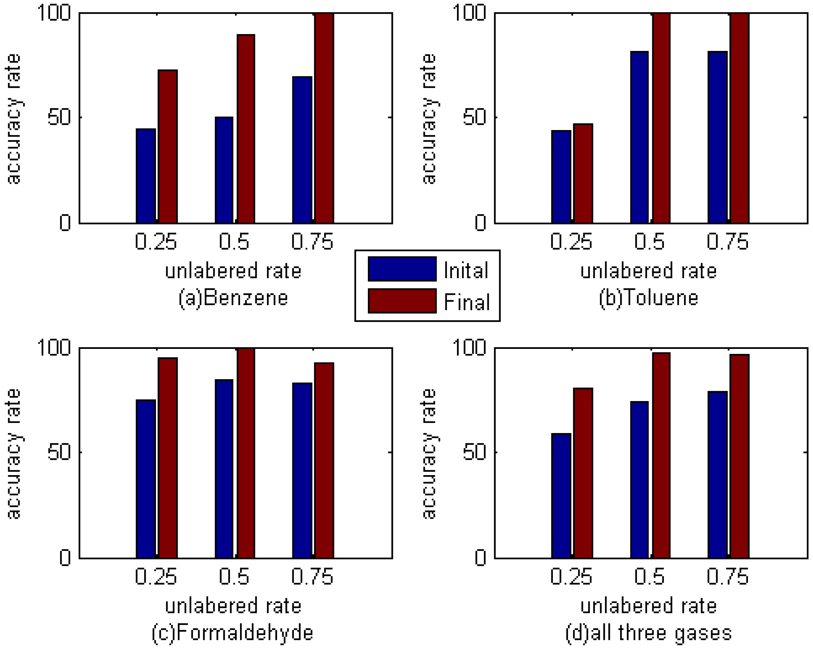
Figure 5 shows the classification accuracy of different gas in the test data set. As can be seen, the recognition rate of these three kinds of gas, whether a single case or all three kinds of gas, has improved in varying degrees. And on the whole, the effect is most obvious when the unlabeled rate is 50%. Whether this is the best proportion is still need to be further verified, but it can be determined that M-training technique can indeed improve the accuracy rate of E-nose to these three kinds of gas.


