
The Local Integrity Approach for Urban Contexts: Definition and Vehicular Experimental Assessment


Abstract
:1. Introduction
- Conventional analytical models used to predict the pseudorange error variances (assuming an open-sky satellite visibility) may be inconsistent for mass-market automotive receivers. In fact the models for the User Equivalent Range Error (UERE) are based on line-of-sight propagation with diffuse ground multipath only, and they often assume the availability of differential corrections. They do not account for possible time- and space-varying impairments (e.g., limited satellite visibility, non-line-of-sight signals, fast fading), whose probability of occurrence is high in urban scenarios [2];
- Typical requirements of integrity and continuity risks associated to aviation operations per phase of flight could be too conservative with respect to the requirements of vehicular applications, especially in non-SoL cases [3];
- In the case of Satellite-Based Augmentation System (SBAS, for example EGNOS in Europe), the typical availability and applicability of GNSS integrity information can be limited in urban canyons. In detail, either the geostationary satellites can be blocked or the obtained PLs can result too conservative for a non-SoL vehicular application (e.g., as demonstrated by the measurement campaigns reported in [6]);
- The classic integrity approach does not take advantage of collaborative architectures, implying the potential availability of additional information from multiple GNSS receivers connected by Vehicle-to-Vehicle and Vehicle-to-Infrastructure communications (e.g., in a VANET) [5].
2. Local GNSS Integrity Approach
2.1. General Idea and Suitable Architecture
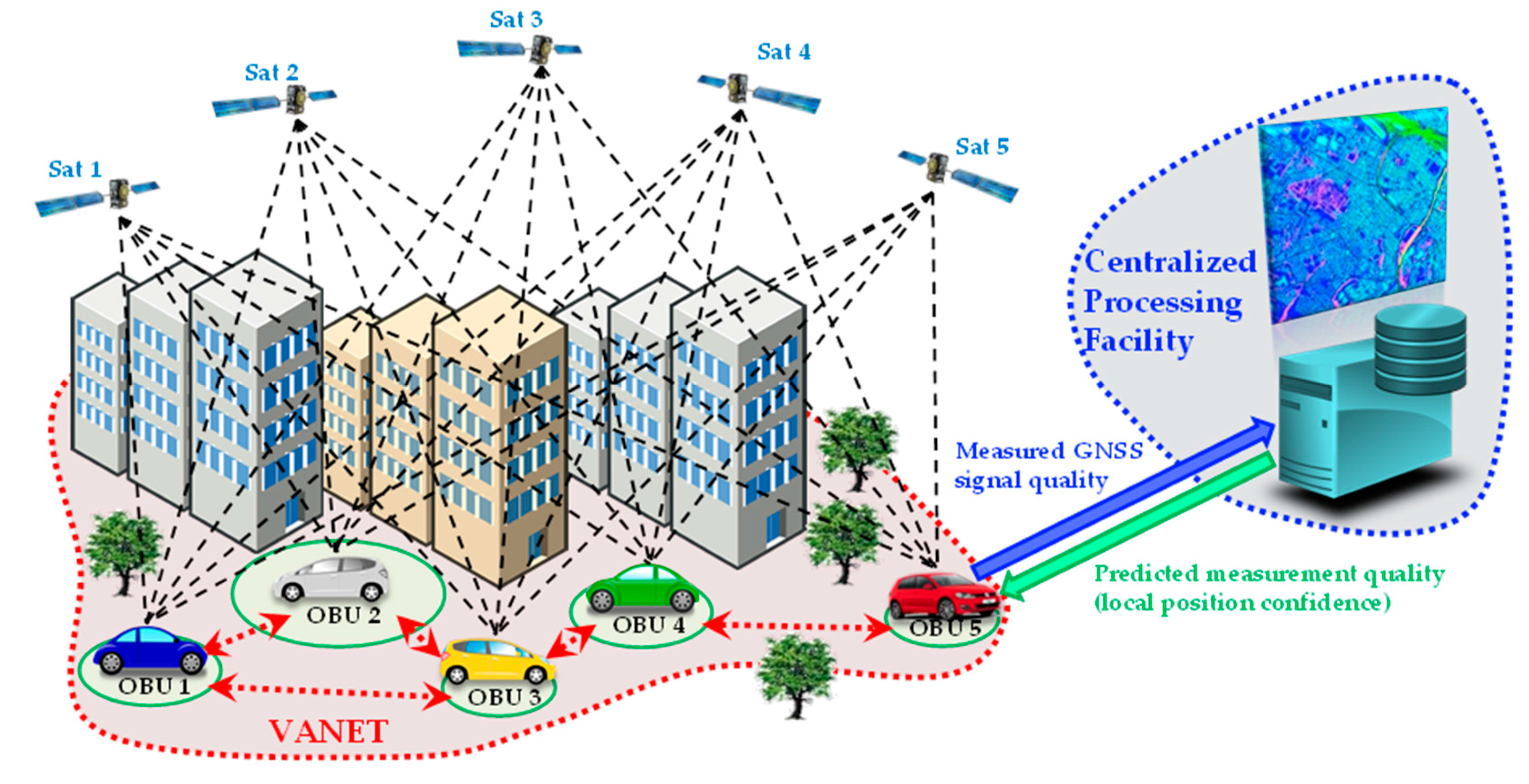
- a (fully or partial) post-processing-based approach, in case of insufficient or intermittent connectivity of the vehicles with the centralized processing facility. In this case GNSS measurements are temporarily stored on board of each vehicle. They are downloaded and transmitted to the server only when the vehicle is connected to the network (e.g., once per day or per month). The suitability of this non-real time approach depends on the application requirements (e.g., in case of a road tolling solution);
- a server-side implementation, requiring one-way communications from the vehicles to the control centre, with centralized processing and without on-board data storage and display (e.g., fleet management);
- a vehicle-side real-time implementation, requiring a two-way communication in order to also display local integrity information on-board of each vehicle (useful for example in a collision avoidance system);
- a completely de-centralized approach, based on a collaborative architecture without the need for a control centre (e.g., in case of info-mobility solutions for leisure applications).
2.2. Exploitation of Pseudorange Residual Measurements
- is the vector containing the differences between nominal (geometrical) ranges and pseudoranges (observations) measured at the n-th time instant for each i-th satellite (with i ranging from 1 to Nsat);
- is the linear connection matrix , derived from the linearization of the PVT solution problem about the selected linearization point;
- is a vector containing the position-time deviation obtained after the LS solution at the n-th time instant [15].
2.3. Effective UERE and Local Protection Levels
- Collect M independent observations of the vector of pseudorange residuals (with n = 1, …, M) from a set of Nsat satellites used in PVT solution. The observations are obtained from different closely-spaced receivers in the VANET and/or combining measurements performed in different days, but with nearly the same geometrical conditions, velocity, and then similar signal degradations.
- Compute the ensemble mean of the covariance matrix of the residuals as:where it must be noted that is a square matrix representing an instantaneous estimate of the covariance matrix at the n-th time instant.
- Estimate the effective UERE variance , starting from the Frobenius-norm of (i.e., the square rooted trace of ) and the number of satellites Nsat.
- Obtain the effective UERE standard deviation as:

3. Experimental Validation and Data Analysis
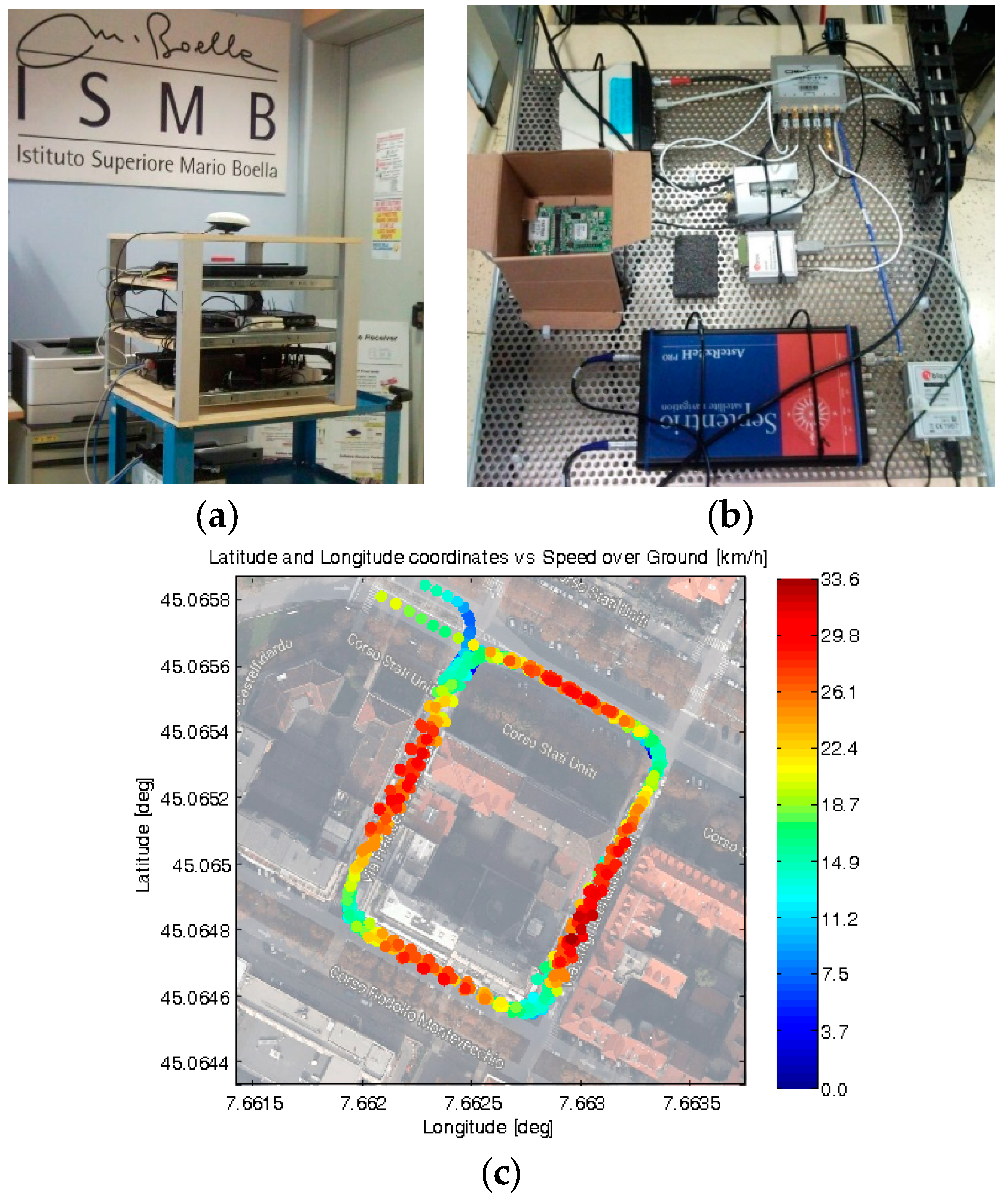
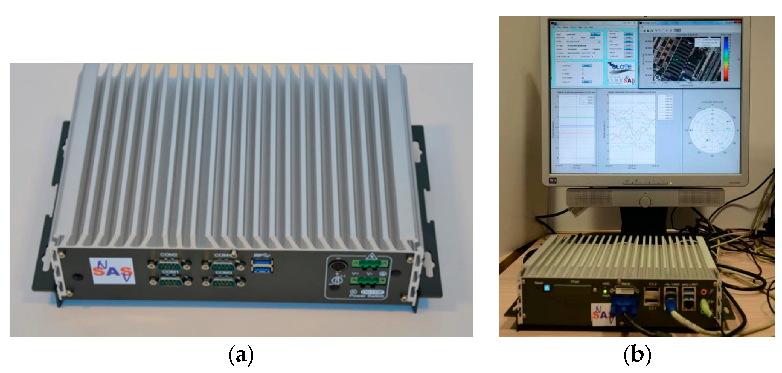
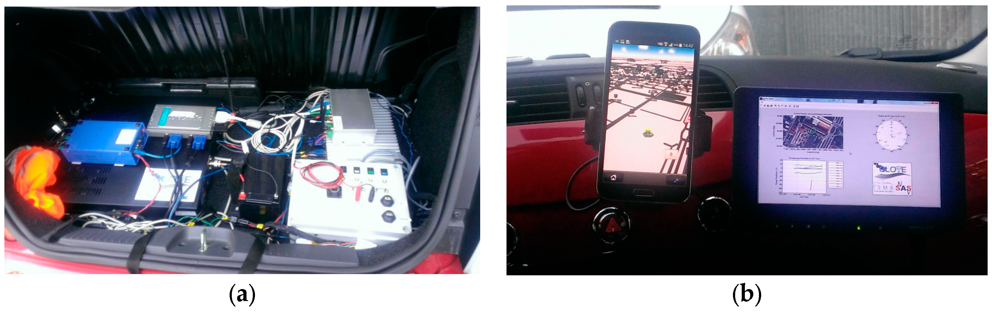
3.1. Measurement Setup and Vehicular Data Collections
3.2. Post-Processing Analyses for Effective UERE Estimation
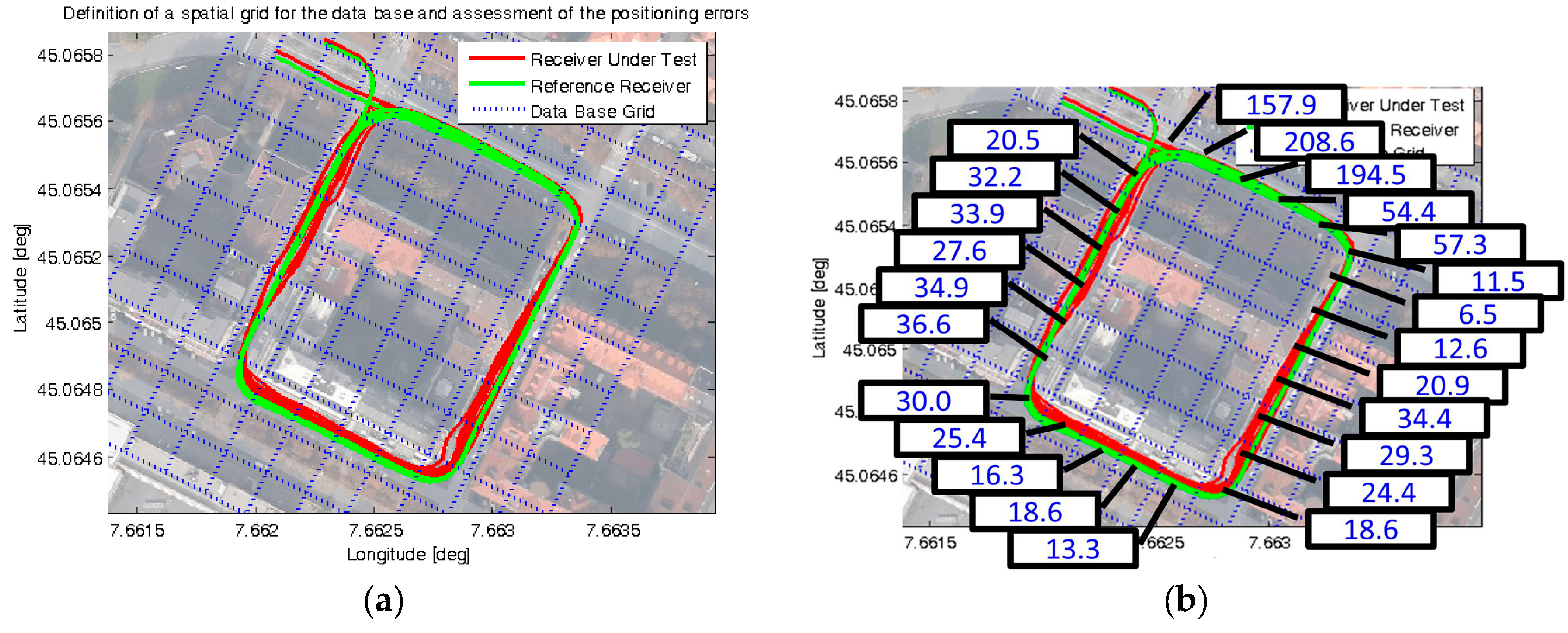
3.3. Computation of the Local Protection Levels

3.4. Simplified UERE Model for Demonstration Purposes


4. Proof-of-Concept and Demonstration Results
4.1. Proof-of-Concept Implementation for Live Demonstration
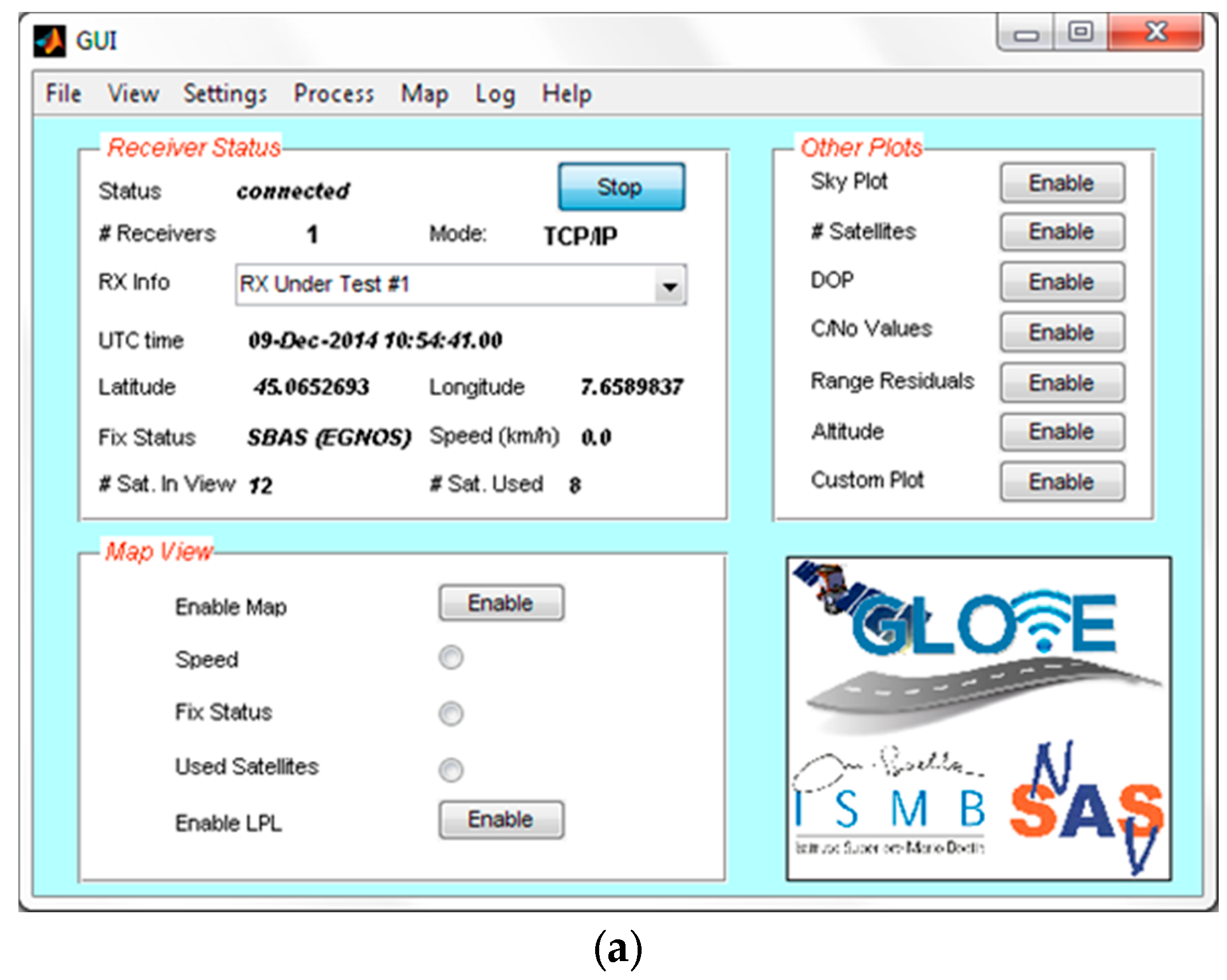
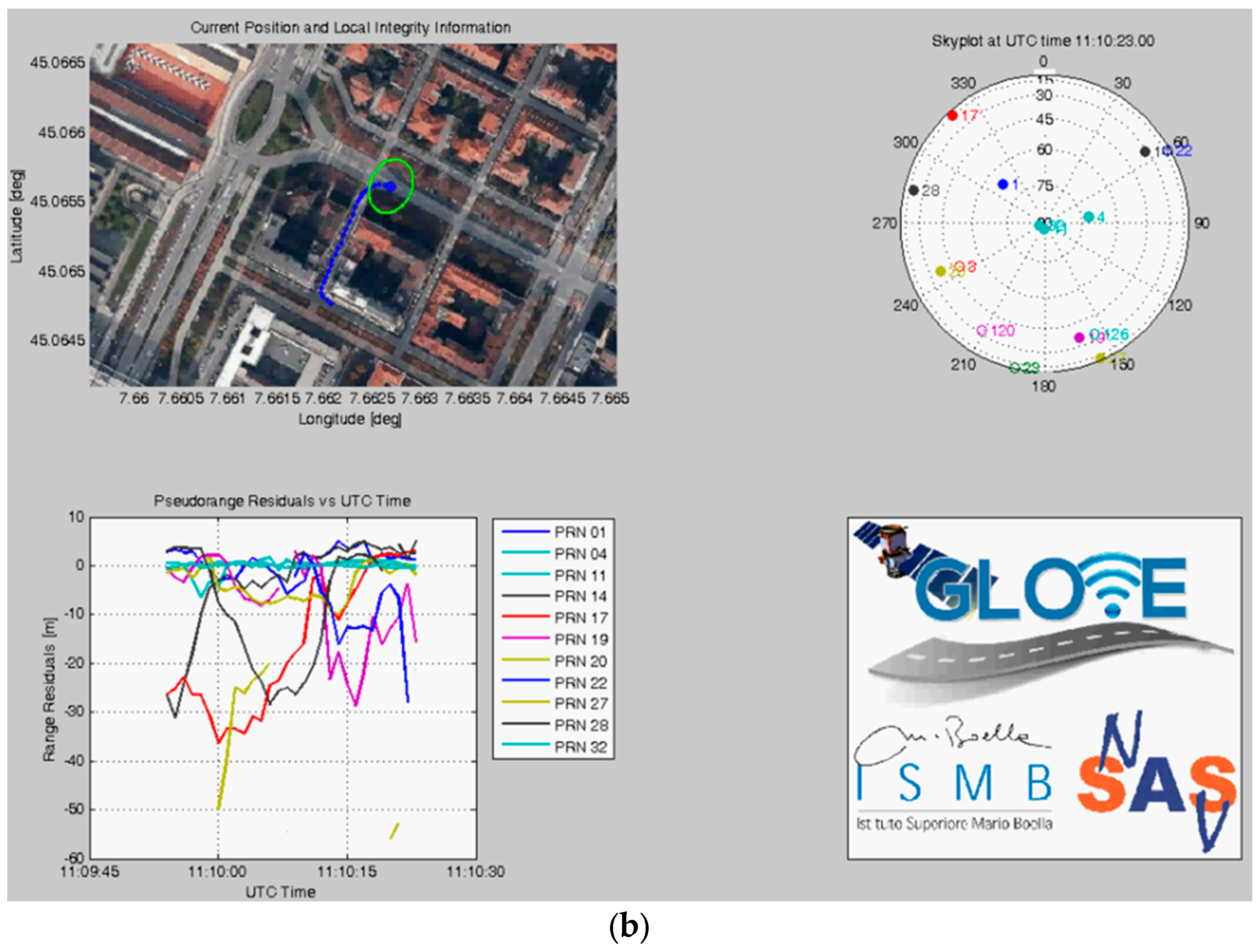
4.2. Prototype Demonstrator of the Local Integrity
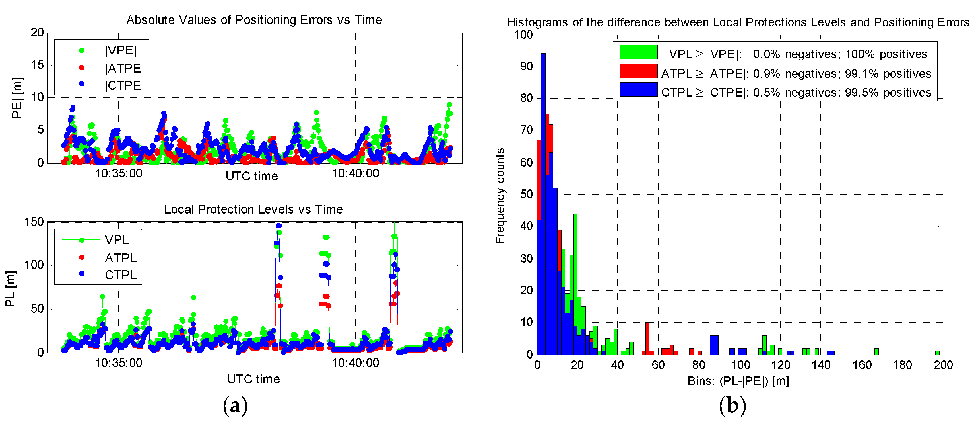
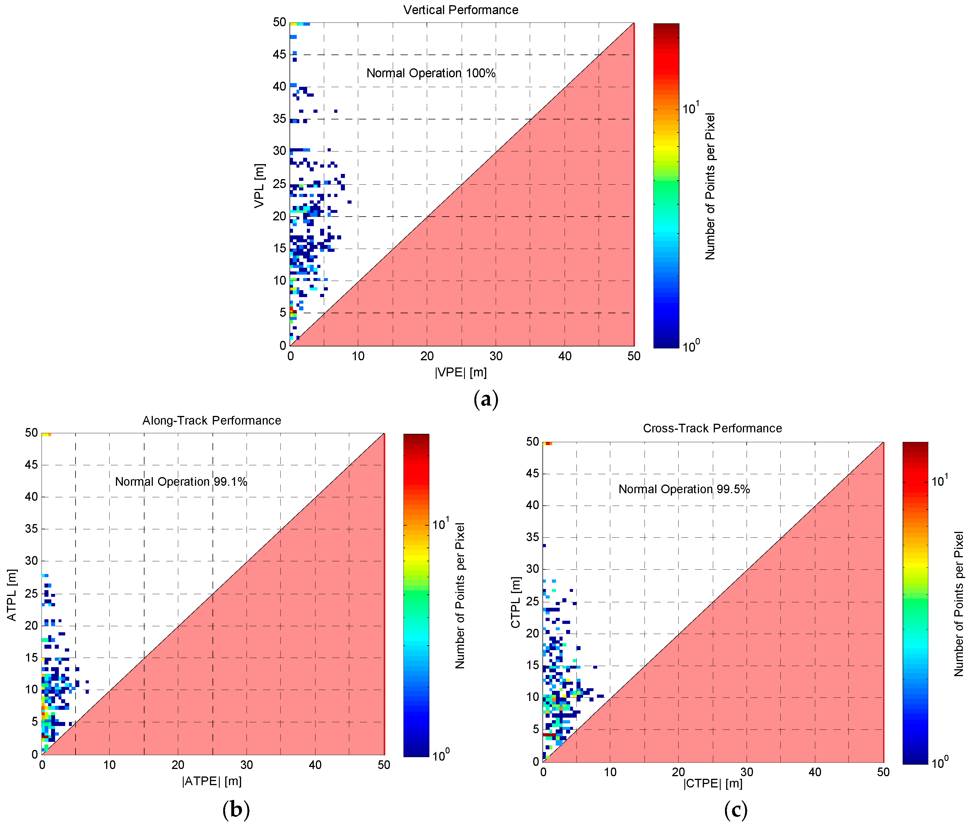
4.3. Obtained Results and Performance Assessment
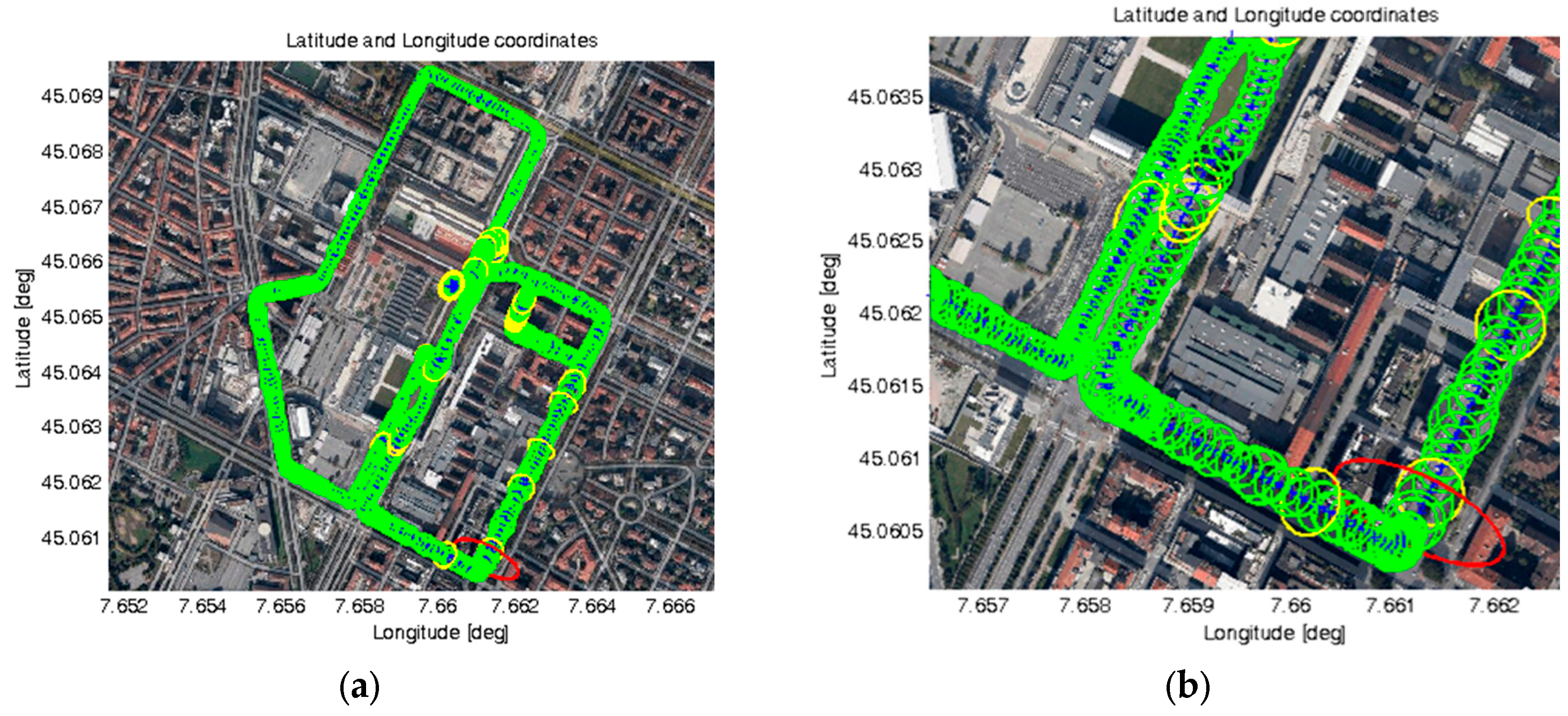

- Green, if such LPL value is below 25 m,
- Yellow, if between 25 and 39 m, and
- Red, if greater than 39 m.

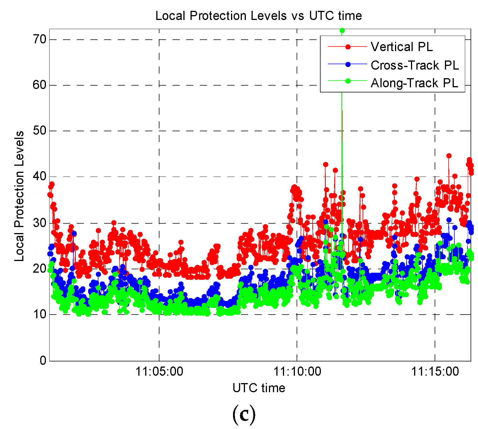
| Directions | Max. PL Value | 95% Quantiles |
|---|---|---|
| Along-Track | 72.1 m | 20.9 m |
| Cross-Track | 30.8 m | 24.7 m |
| Vertical | 72.3 m | 36.3 m |
5. Conclusions
Acknowledgments
Author Contributions
Conflicts of Interest
Abbreviations
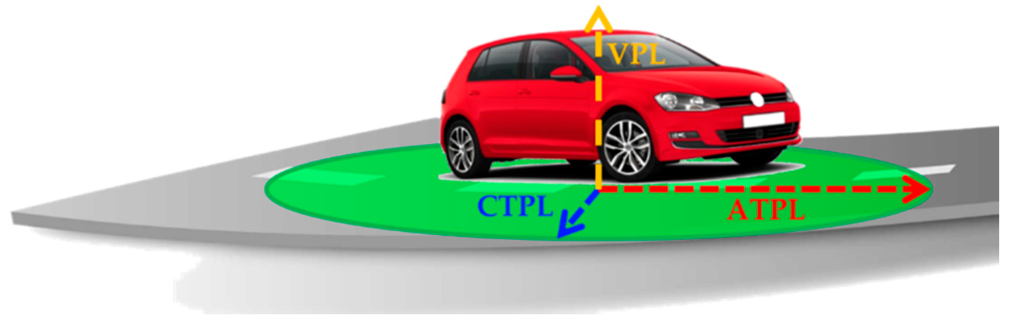
| ACU: | Along-Track, Cross-Track, Up |
| AT: | Along-Track |
| C/N0: | Carrier-to-Noise density ratio |
| CC-BY: | Creative Commons by Attribution |
| CT: | Cross-Track |
| EGNOS: | European Geostationary Navigation Overlay Service |
| GBAS: | Ground-Based Augmentation System |
| GLOVE: | joint GaliLeo Optimization and VANET Enhancement |
| GNSS: | Global Navigation Satellite System |
| GPS: | Global Positioning System |
| GUI: | Graphical User Interface |
| IMU: | Inertial Measurement Unit |
| ISMB: | Istituto Superiore Mario Boella |
| LPL: | Local Protection Level |
| LS: | Least Squares |
| MDPI: | Multidisciplinary Digital Publishing Institute |
| NMEA: | National Marine Electronics Association |
| OBU: | On-Board Unit |
| PE: | Positioning Error |
| PL: | Protection Level |
| PVT: | Position, Velocity, and Time |
| RAIM: | Receiver Autonomous Integrity Monitoring |
| RTK: | Real Time Kinematic |
| SBAS: | Satellite-Based Augmentation System |
| SoL: | Safety-of-Life |
| UERE: | User Equivalent Range Error |
| USB: | Universal Serial Bus |
| V: | Vertical |
| VANET: | Vehicular Ad hoc NETwork |
References
- Rife, J.; Pullen, S. Aviation applications (Chapter 10). In GNSS Applications and Methods, 1st ed.; Gleason, S., Gebre-Egziabher, D., Eds.; Artech House: Norwood, MA, USA, 2009; pp. 245–268. [Google Scholar]
- Cosmen-Schortmann, J.; Azaola-Saenz, M.; Martinez-Olague, M.A.; Toledo-Lopez, M. Integrity in Urban and Road Environments and its Use in Liability Critical Applications. In Proceedings of the IEEE/ION Position, Location and Navigation Symposium, Monterey, CA, USA, 5–8 May 2008; pp. 972–983.
- Pullen, S.; Walter, T.; Enge, P. SBAS and GBAS Integrity for Non-Aviation Users: Moving Away from “Specific Risk”. In Proceedings of the 2011 International Technical Meeting of The Institute of Navigation, San Diego, CA, USA, 24–26 January 2011; pp. 533–545.
- Scopigno, R.; Margaria, D.; Acarman, T.; Peker, A.U.; Par, K.; Kaplan, E. GLOVE’s Manifesto: Leveraging GNSS Time-Space Information to Improve VANETs’ Performances and Enrich VANETs’ Services. In Proceedings of the 9th ITS European Congress, Dublin, Ireland, 4–7 June 2013; pp. 1–12.
- Margaria, D.; Falletti, E.; Acarman, T. The Need for GNSS Position Integrity and Authentication in ITS: Conceptual and Practical Limitations in Urban Contexts. In Proceedings of the 2014 IEEE Intelligent Vehicles Symposium (IV’14), Dearborn, MI, USA, 8–11 June 2014; pp. 1384–1389.
- Ali, K.; Pini, M.; Dovis, F. Measured Performance of the Application of EGNOS in the Road Traffic Sector. GPS Solut. 2012, 16, 135–145. [Google Scholar] [CrossRef]
- Lee, B.-H.; Song, J.-H.; Im, J.-H.; Im, S.-H.; Heo, M.-B.; Jee, G.-I. GPS/DR Error Estimation for Autonomous Vehicle Localization. Sensors 2015, 15, 20779–20798. [Google Scholar] [CrossRef] [PubMed]
- Carmona, J.; García, F.; Martín, D.; Escalera, A.; Armingol, J.M. Data Fusion for Driver Behaviour Analysis. Sensors 2015, 15, 25968–25991. [Google Scholar] [CrossRef] [PubMed]
- Gu, Y.; Hsu, L.-T.; Kamijo, S. Passive Sensor Integration for Vehicle Self-Localization in Urban Traffic Environment. Sensors 2015, 15, 30199–30220. [Google Scholar] [CrossRef] [PubMed]
- Margaria, D.; Falletti, E. A Novel Local Integrity Concept for GNSS Receivers in Urban Vehicular Contexts. In Proceedings of the IEEE/ION Position, Location and Navigation Symposium, Monterey, CA, USA, 5–8 May 2014; pp. 413–425.
- Margaria, D.; Falletti, E. The Local GNSS Integrity Concept: Feasibility and Experimental Validation in an Urban Vehicular Scenario. In Proceedings of the 7th ESA Workshop on Satellite Navigation Technologies (NAVITEC 2014), Noordwijk, The Netherlands, 3–5 December 2014; pp. 621–627.
- GSA—Local Integrity: Characterization of GNSS Degradations in Urban Scenarios. Available online: http://www.gsa.europa.eu/news/local-integrity-characterization-gnss-degradations-urban-scenarios (accessed on 26 November 2015).
- Margaria, D.; Falletti, E. Proof-of-concept of the Local Integrity Approach: Prototype Implementation and Performance Assessment in an Urban Context. In Proceedings of the 2015 International Conference on Localization and GNSS (ICL-GNSS), Gothenburg, Sweden, 22–24 June 2015. [CrossRef]
- Borre, K. GPS EASY suite II, easy13—RAIM. Inside GNSS 2009, 4, 48–51. [Google Scholar]
- Kaplan, E.D.; Hegarty, C.J. Understanding GPS: Principles and Applications, 2nd ed.; Artech House: Norwood, MA, USA, 2006; pp. 54–63. [Google Scholar]
- U-Blox 6 Evaluation Kits. Available online: https://www.u-blox.com/en/product/evk-6 (accessed on 26 November 2015).
- National Marine Electronics Association—NMEA. Available online: http://www.nmea.org/ (accessed on 26 November 2015).
- European Space Agency Navipedia—Galileo Space Segment. Available online: http://www.navipedia.net/index.php/Galileo_Space_Segment (accessed on 26 November 2015).
- Borre, K. GPS EASY suite II, easy14—EGNOS-aided aviation. Inside GNSS 2009, 4, 62–66. [Google Scholar]
- GLOVE Project—Joint Galileo Optimization and VANET Enhancement. Available online: http://www.gsa.europa.eu/joint-galileo-optimization-and-vanet-enhancement (accessed on 22 January 2016).
© 2016 by the authors; licensee MDPI, Basel, Switzerland. This article is an open access article distributed under the terms and conditions of the Creative Commons by Attribution (CC-BY) license (http://creativecommons.org/licenses/by/4.0/).
Share and Cite
Margaria, D.; Falletti, E. The Local Integrity Approach for Urban Contexts: Definition and Vehicular Experimental Assessment. Sensors 2016, 16, 154. https://doi.org/10.3390/s16020154
Margaria D, Falletti E. The Local Integrity Approach for Urban Contexts: Definition and Vehicular Experimental Assessment. Sensors. 2016; 16(2):154. https://doi.org/10.3390/s16020154
Chicago/Turabian StyleMargaria, Davide, and Emanuela Falletti. 2016. "The Local Integrity Approach for Urban Contexts: Definition and Vehicular Experimental Assessment" Sensors 16, no. 2: 154. https://doi.org/10.3390/s16020154