
Optical Microbubble Resonators with High Refractive Index Inner Coating for Bio-Sensing Applications: An Analytical Approach

 ,
,  ,
,  ,
,  ,
,  and
and 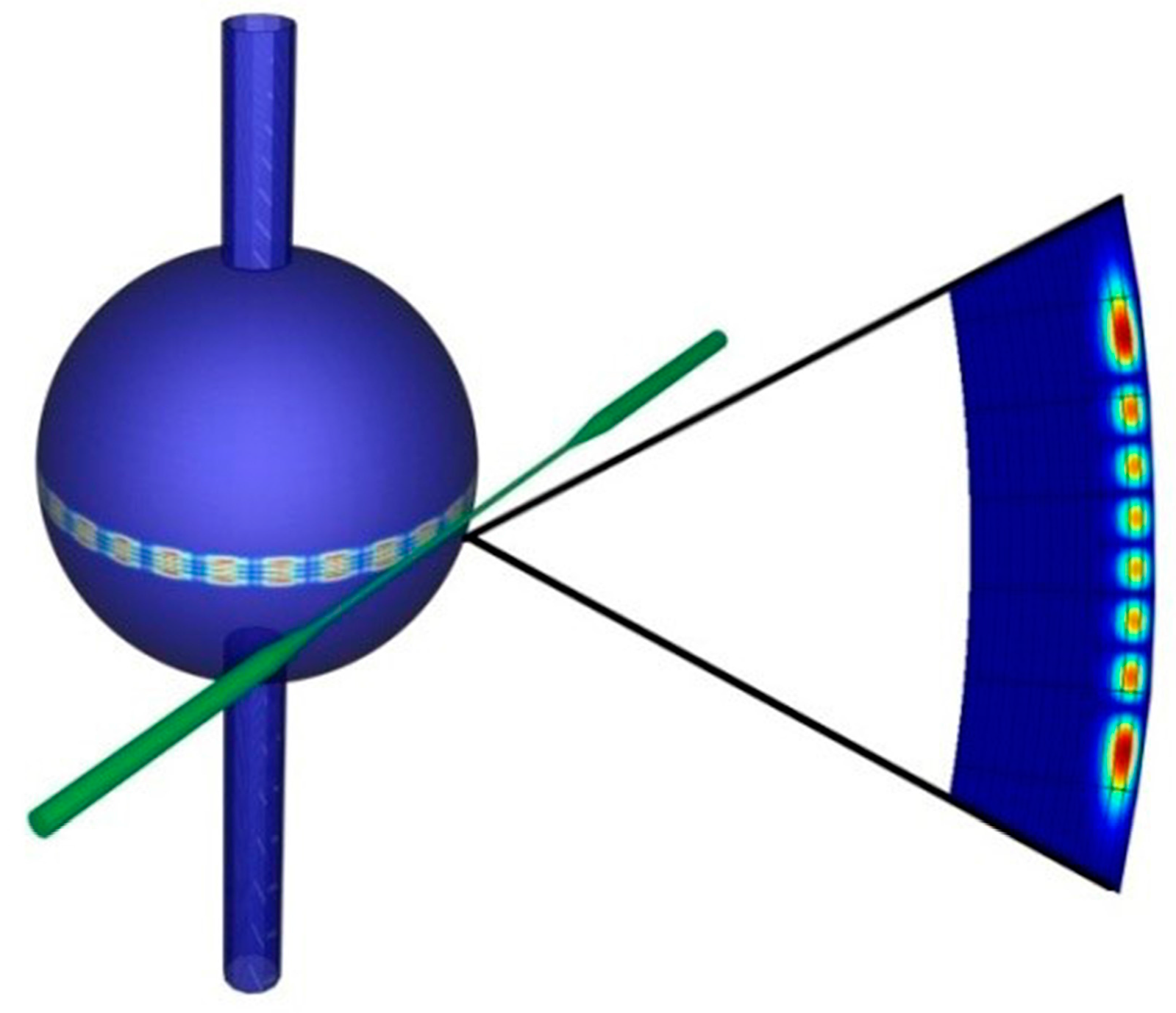
Abstract
:1. Introduction
2. Methods
2.1. OMBR Analytical Model
- l is the azimuthal mode number and it is linked to the max.–min. number of the periodical functions sin(x) and cos(x) along the equatorial plane;
- m is the polar mode number and it is related to the max.−min. number of the harmonic Legendre functions in the polar direction (n° max. in the polar direction: l − m + 1); and
- n is associated to the max.–min. number of the field in the radial direction.
| 0 | 0 | 0 | 0 | 0 | |||
| 0 | 0 | 0 | 0 | 0 | |||
| 0 | 0 | 0 | 0 | ||||
| 0 | 0 | 0 | 0 | ||||
| 0 | 0 | 0 | 0 | ||||
| 0 | 0 | 0 | 0 | ||||
| 0 | 0 | 0 | 0 | 0 | |||
| 0 | 0 | 0 | 0 | 0 |
2.2. OMBR Sensitivity
2.3. OMBR Limit of Detection
3. Results and Discussion
3.1. Sensitivity for an OMBR without Inner Polymeric Coating
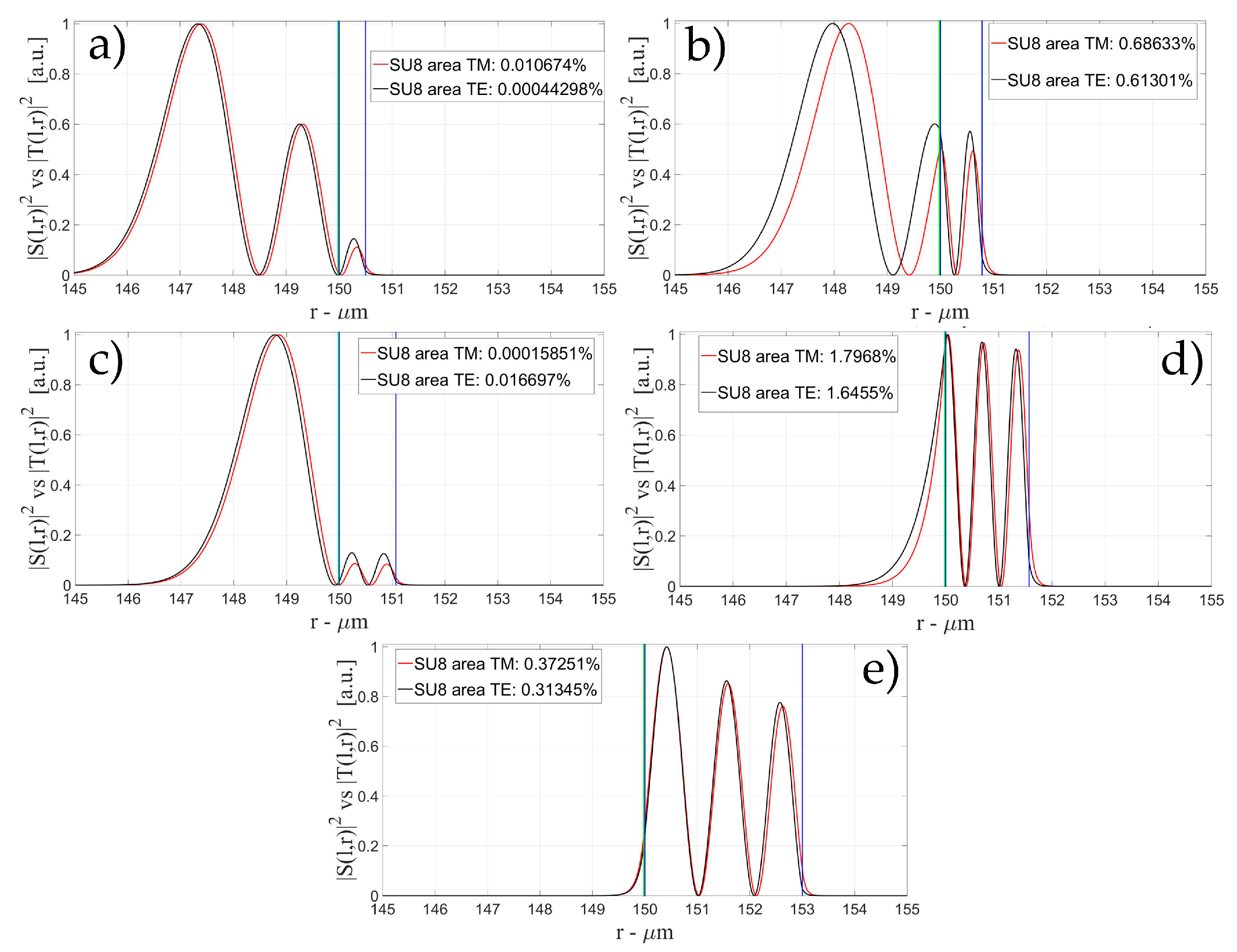
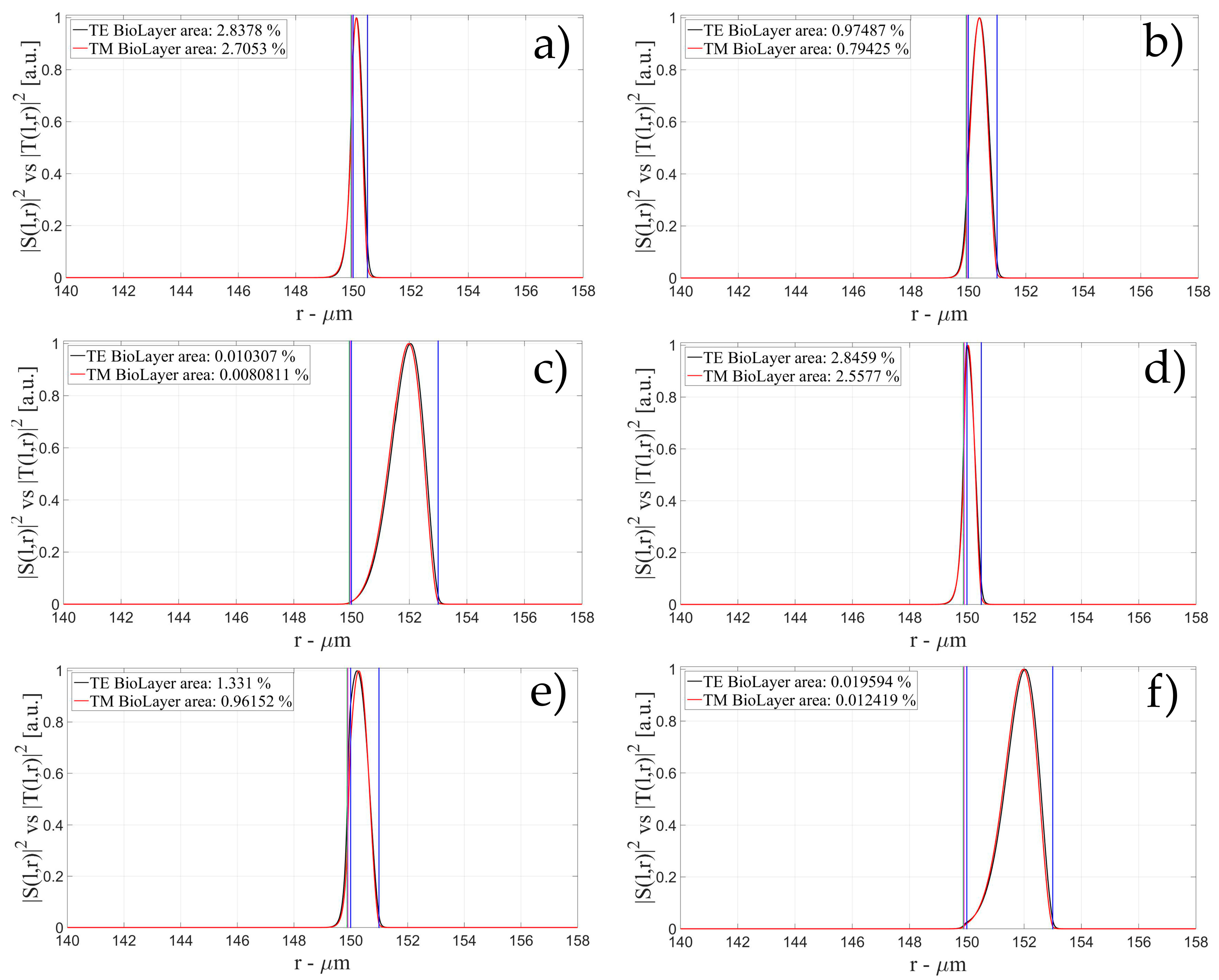
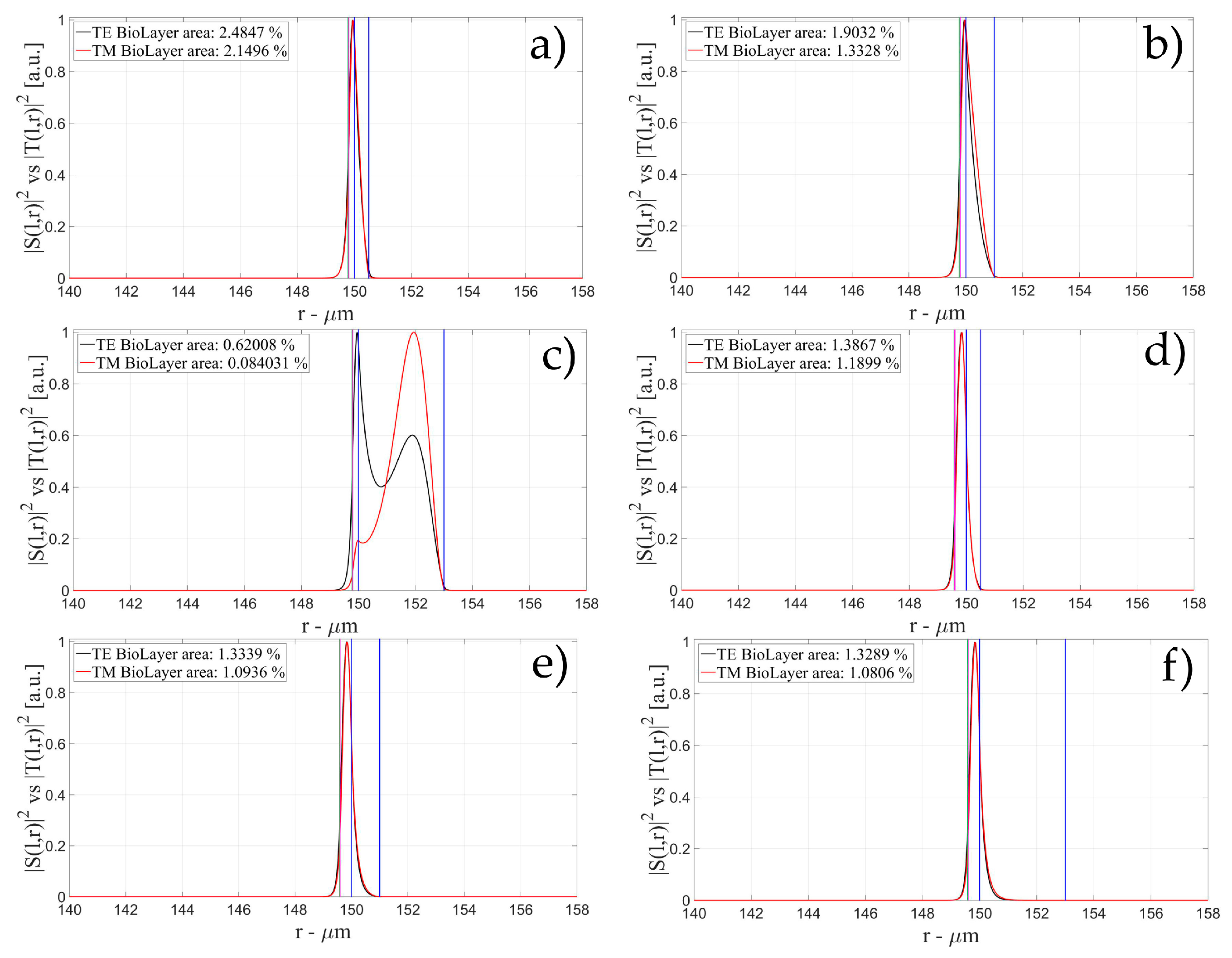
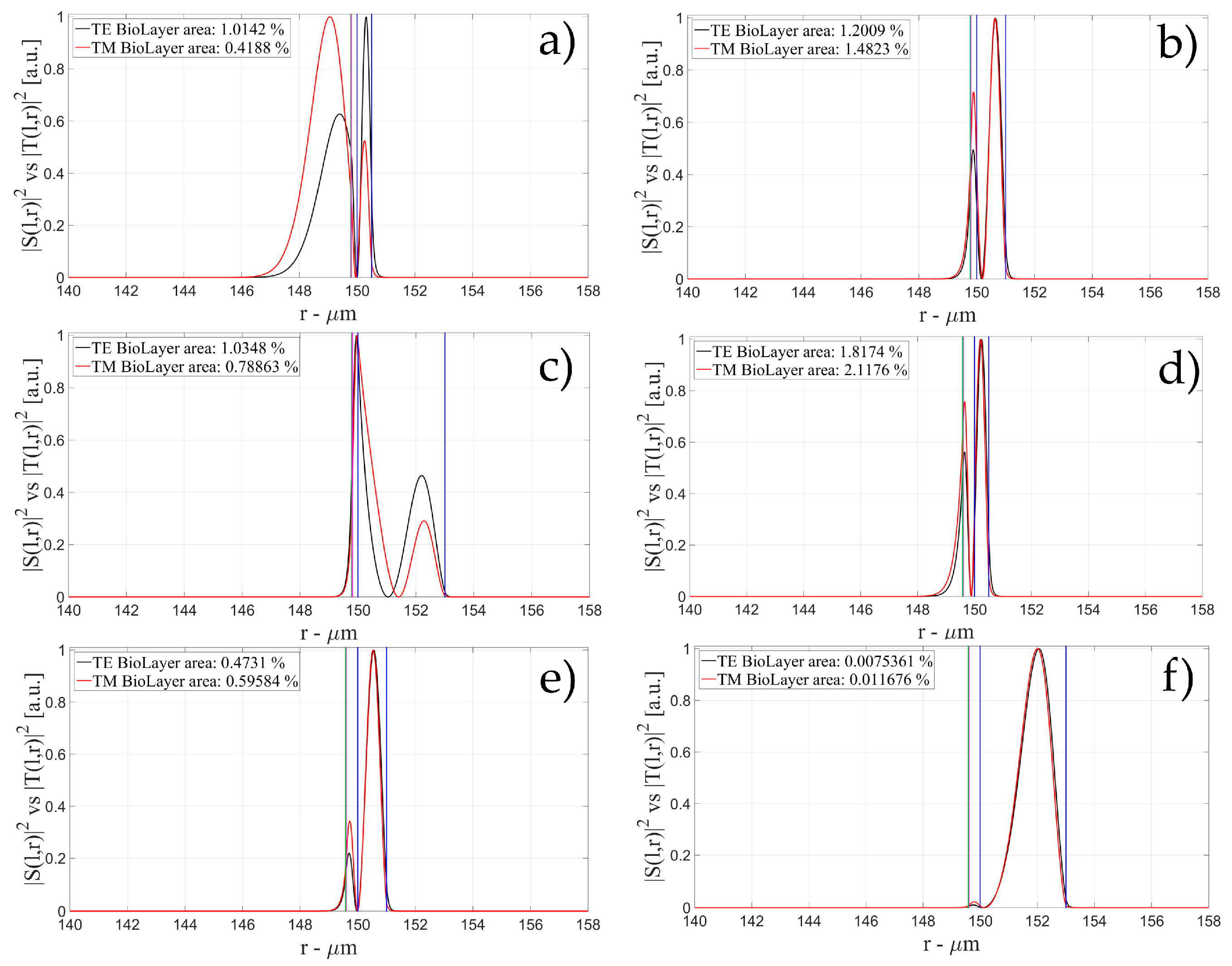
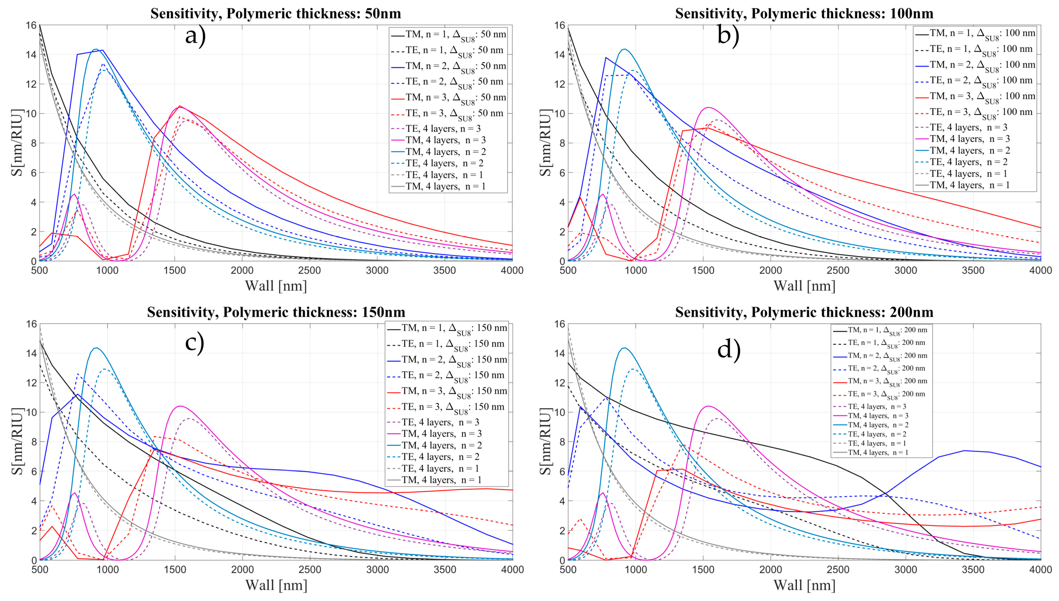
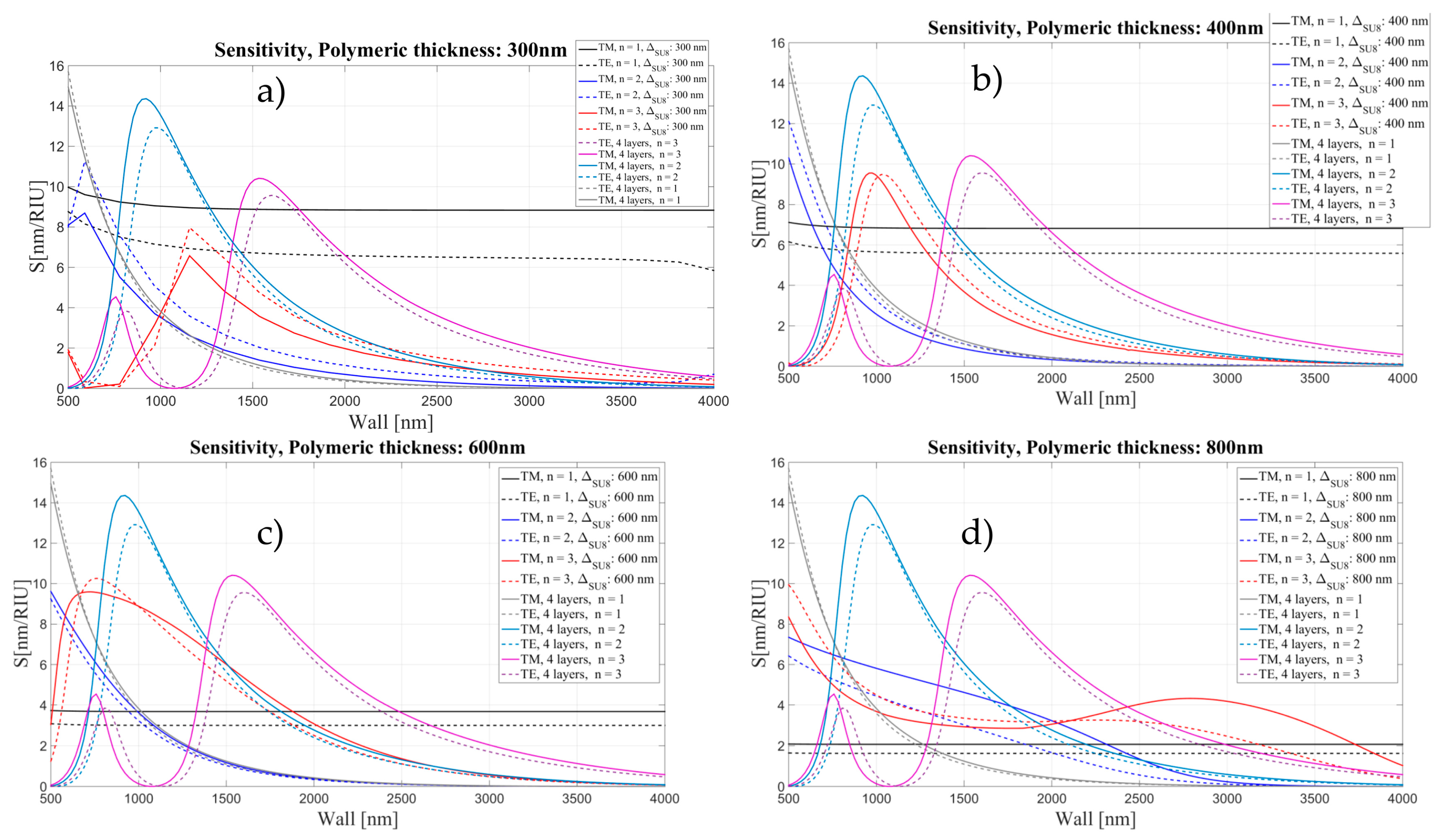
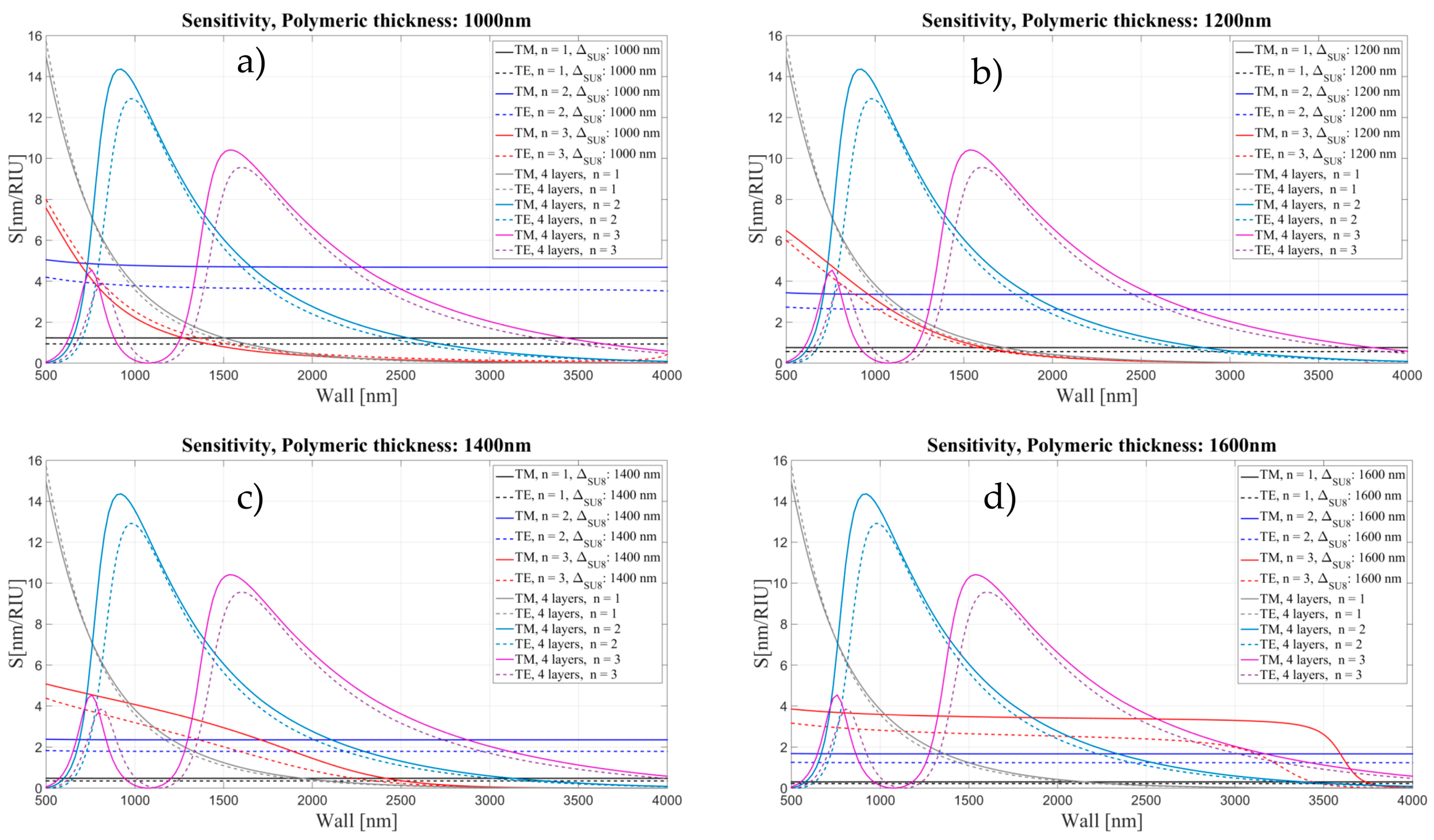
3.2. Sensitivity for an OMBR with an Inner Polymeric Coating
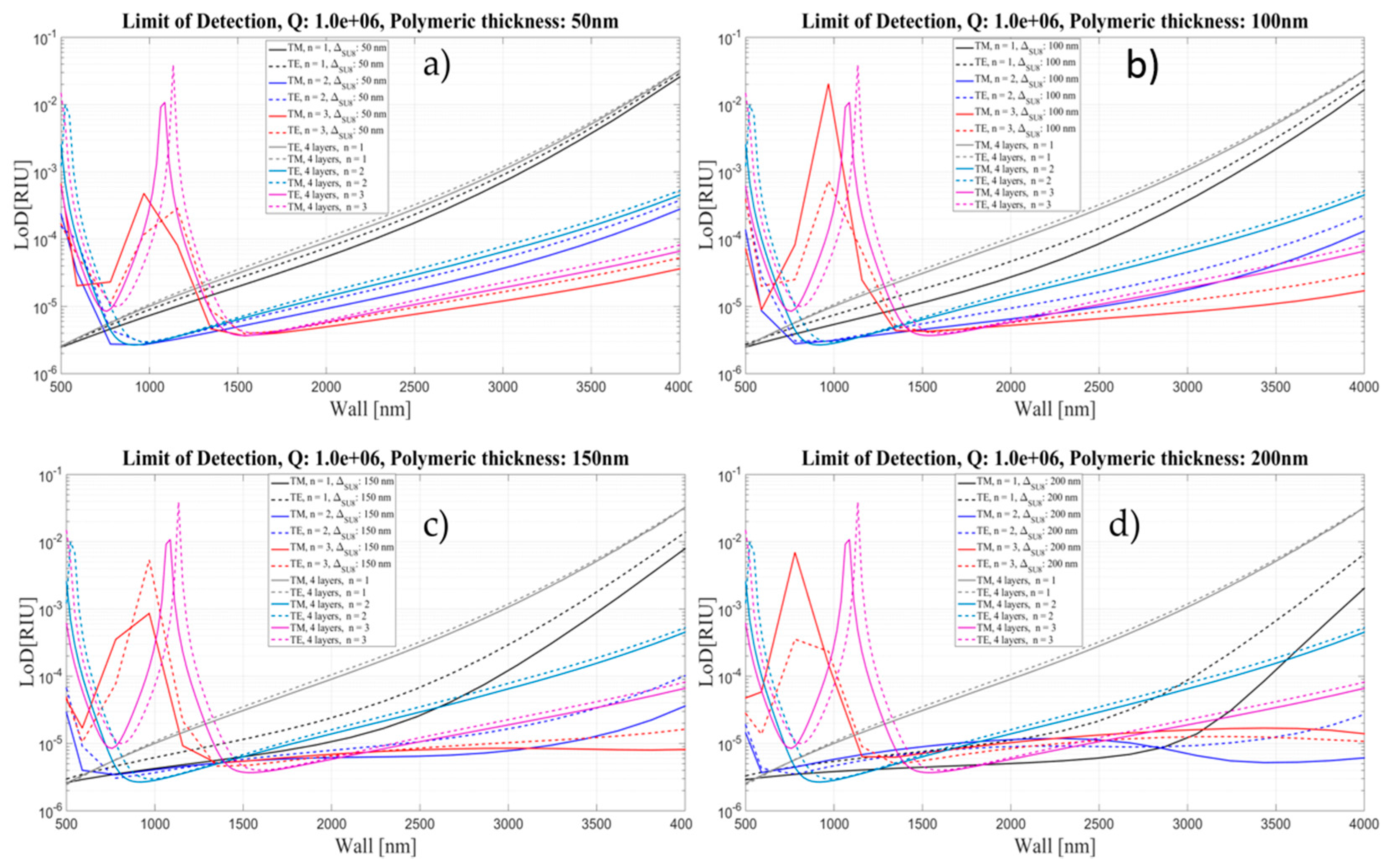
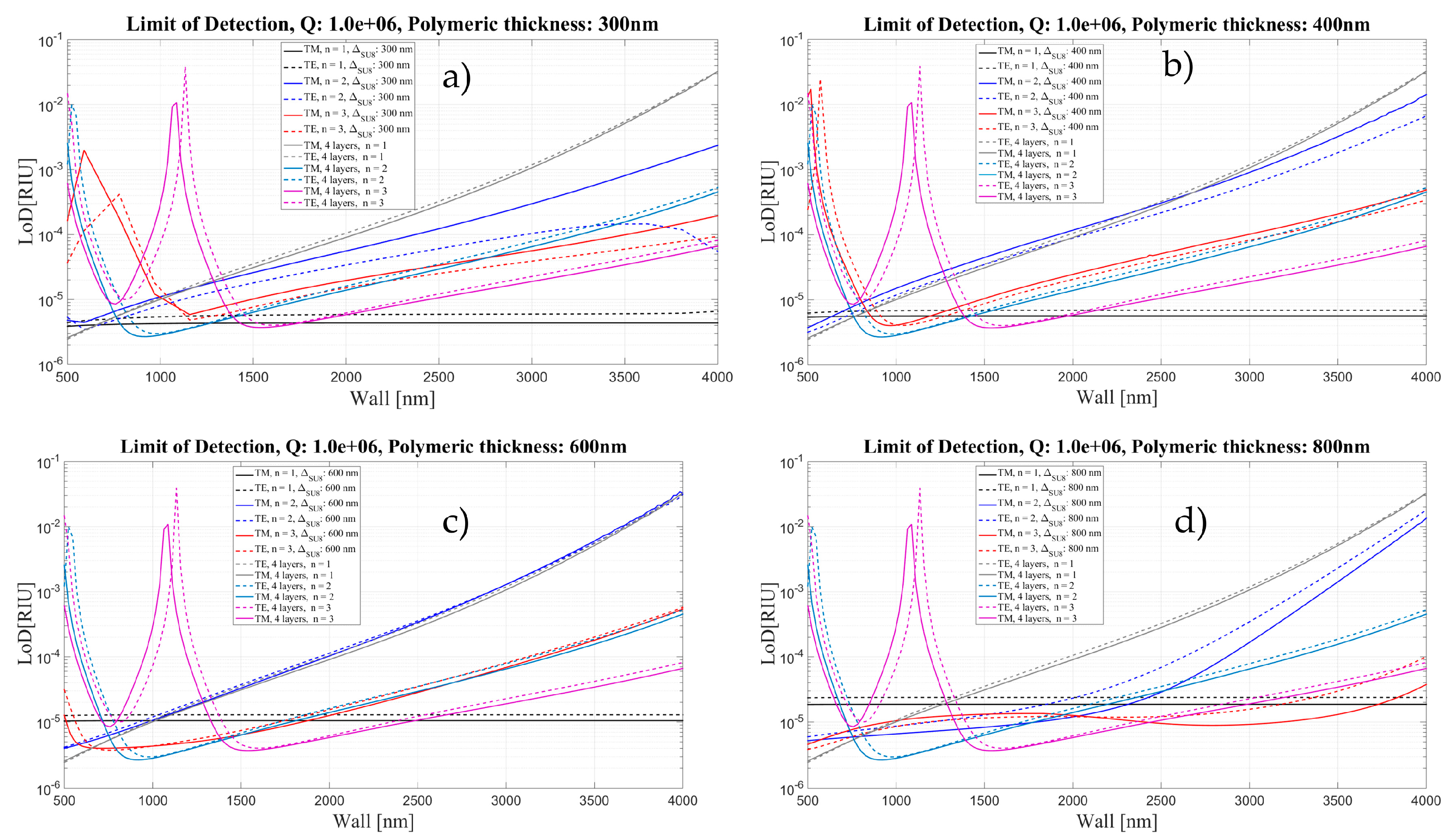
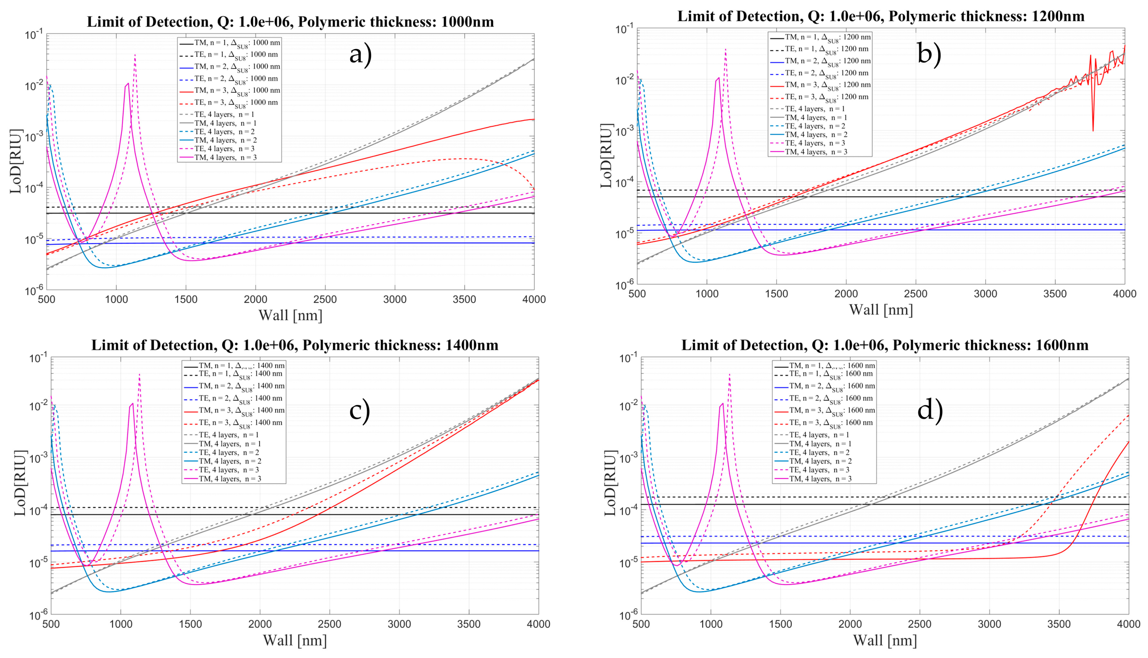
4. Limit of Detection
5. Conclusions
Acknowledgments
Author Contributions
Conflicts of Interest
References
- Reynolds, T.; Henderson, M.R.; François, A.; Riesen, N.; Hall, J.M.M.; Afshar, S.V.; Nicholls, S.J.; Monro, T.M. Optimization of whispering gallery resonator design for biosensing applications. Opt. Express 2015, 23, 17067–17076. [Google Scholar] [CrossRef] [PubMed]
- Lin, N.; Jiang, L.; Wang, S.; Chen, Q.; Xiao, H.; Lu, Y.; Tsai, H. Simulation and optimization of polymer-coated microsphere resonators in chemical vapor sensing. Appl. Opt. 2011, 50, 5465–5472. [Google Scholar] [CrossRef] [PubMed]
- Soria, S.; Berneschi, S.; Brenci, M.; Cosi, F.; Nunzi Conti, G.; Pelli, S.; Righini, G.C. Optical Microspherical Resonators for Biomedical Sensing. Sensors 2011, 11, 785–805. [Google Scholar] [CrossRef] [PubMed]
- Tan, W.; Shi, L.; Chen, X. Modeling of an optical sensor based on whispering gallery modes (WGMs) on the surface guiding layer of glass filaments. Sensors 2008, 8, 6761–6768. [Google Scholar] [CrossRef] [PubMed]
- Boleininger, A.; Lake, T.; Hami, S.; Vallance, C. Whispering gallery modes in standard optical fibres for fibre profiling measurements and sensing of unlabeled chemical species. Sensors 2010, 10, 1765–1781. [Google Scholar] [CrossRef] [PubMed]
- Chantada, L.; Nikolaev, N.I.; Ivanov, A.L.; Borri, P.; Langbein, W. Optical resonances in microcylinders: Response to perturbations for biosensing. J. Opt. Soc. Am. B 2008, 25, 1312–1321. [Google Scholar] [CrossRef]
- Boyd, R.W.; Heebner, J.E. Sensitive disk resonator photonic biosensor. Appl. Opt. 2001, 40, 5742–5747. [Google Scholar] [CrossRef] [PubMed]
- Lipka, T.; Wahn, L.; Trieu, H.K.; Hilterhaus, L.; Muller, J. Label-free photonic biosensors fabricated with low-loss hydrogenated amorphous silicon resonators. J. Nanophotonics 2013, 7, 073793. [Google Scholar] [CrossRef]
- Wang, F.; Anderson, M.; Bernards, M.T.; Hunt, H.K. PEG Functionalization of Whispering Gallery Mode Optical Microresonator Biosensors to Minimize Non-Specific Adsorption during Targeted, Label-Free Sensing. Sensors 2015, 15, 18040–18060. [Google Scholar] [CrossRef] [PubMed]
- Ozgur, E.; Toren, P.; Aktas, O.; Huseyinoglu, E.; Bayindir, M. High selectivity label-free biosensing in complex media using microtoroidal resonators. Sci. Rep. 2015, 5, 13173. [Google Scholar] [CrossRef] [PubMed] [Green Version]
- White, I.M.; Oveys, H.; Fan, X. Liquid-core optical ring-resonator sensors. Opt. Lett. 2006, 31, 1319–1321. [Google Scholar] [CrossRef] [PubMed]
- Zhu, H.; White, I.M.; Suter, J.D.; Dale, P.S.; Fan, X. Analysis of biomolecule detection with optofluidic ring resonator sensors. Opt. Express 2007, 15, 9139–9146. [Google Scholar] [CrossRef] [PubMed]
- Sun, Y.; Fan, X. Optical ring resonators for biochemical and chemical sensing. Anal. Bioanal. Chem. 2011, 399, 205–211. [Google Scholar] [CrossRef] [PubMed]
- Zamora, V.; Díez, A.; Andrés, M.V.; Gimeno, B. Refractometric sensor based on whispering gallery modes of thin capillaries. Opt. Express 2007, 15, 12011–12016. [Google Scholar] [CrossRef] [PubMed]
- Lin, N.; Jiang, L.; Wang, S.; Xiao, H.; Lu, Y.; Tsai, H.-L. Design and optimization of liquid core optical ring resonator for refractive index sensing. Appl. Opt. 2011, 50, 3615–3621. [Google Scholar] [CrossRef] [PubMed]
- Cho, H.K.; Han, J. Numerical Study of Opto-Fluidic Ring Resonators for Biosensor Applications. Sensors 2012, 12, 14144–14157. [Google Scholar] [CrossRef] [PubMed]
- Sumetsky, M.; Windeler, R.S.; Dulashko, Y.; Fan, X. Optical liquid ring resonator sensor. Opt. Express 2007, 15, 14376–14381. [Google Scholar] [CrossRef] [PubMed]
- Sun, Y.; Fan, X. Analysis of ring resonator for chemical vapor sensor development. Opt. Express 2008, 16, 10254–10268. [Google Scholar] [CrossRef] [PubMed]
- Ling, T.; Jay Guo, L. Sensitivity enhancement in optical micro-tube resonator sensors via mode coupling. Appl. Phys. Lett. 2013, 103, 013702. [Google Scholar] [CrossRef]
- Ling, T.; Jay Guo, L. A unique resonance mode observed in a prism-coupled micro-tube resonator sensor with superior index sensitivity. Opt. Express 2007, 15, 17424–17432. [Google Scholar] [CrossRef] [PubMed]
- Ling, T.; Jay Guo, L. Analysis of the sensing properties of silica microtube resonator sensors. J. Opt. Soc. Am. B 2009, 26, 471–477. [Google Scholar] [CrossRef]
- Lane, S.; Chan, J.; Thiessen, T.; Meldrum, A. Whispering gallery mode structure and refractometric sensitivity of fluorescent capillary-type sensors. Sens. Actuators B Chem. 2014, 190, 752–759. [Google Scholar] [CrossRef]
- Lane, S.; Marsiglio, F.; Zhi, Y.; Meldrum, A. Refractometric sensitivity and thermal stabilization of fluorescent core microcapillary sensors: Theory and experiment. Appl. Opt. 2015, 54, 1331–1340. [Google Scholar] [CrossRef] [PubMed]
- Lane, S.; West, P.; François, A.; Meldrum, A. Protein biosensing with fluorescent microcapillaries. Opt. Express 2015, 23, 2577–2590. [Google Scholar] [CrossRef] [PubMed]
- Rowland, K.J.; Francois, A.; Hoffmann, P.; Monro, T.M. Fluorescent polymer coated capillaries as optofluidic refractometric sensors. Opt. Express 2013, 21, 11493–11505. [Google Scholar] [CrossRef] [PubMed]
- Sumetsky, M.; Dulashko, Y.; Windeler, R.S. Optical microbubble resonator. Opt. Lett. 2010, 35, 898–900. [Google Scholar] [CrossRef] [PubMed]
- Ward, J.M.; Dhasmana, N.; Nic Chormaic, S. Hollow core, whispering gallery resonator sensors. Eur. Phys. J. Spec. Top. 2014, 223, 1917–1935. [Google Scholar] [CrossRef]
- Berneschi, S.; Farnesi, D.; Cosi, F.; Nunzi Conti, G.; Pelli, S.; Righini, G.C.; Soria, S. High Q silica microbubble resonators fabricated by arc discharge. Opt. Lett. 2011, 36, 3521–3523. [Google Scholar] [CrossRef] [PubMed]
- Yang, Y.; Saurabh, S.; Ward, J.M.; Nic Chormaic, S. High Q, ultrathin-walled microbubble resonator for aerostatic pressure sensing. Opt. Express 2016, 24, 294–299. [Google Scholar] [CrossRef] [PubMed]
- Li, H.; Guo, Y.; Sun, Y.; Reddy, K.; Fan, X. Analysis of single nanoparticle detection by using 3-dimensionally confined optofluidic ring resonator. Opt. Express 2010, 18, 25081–25088. [Google Scholar] [CrossRef] [PubMed]
- Yang, Y.; Ward, J.; Nic Chormaic, S. Quasi-droplet microbubbles for high resolution sensing applications. Opt. Express 2014, 22, 6881–6898. [Google Scholar] [CrossRef] [PubMed]
- Ward, J.M.; Yang, Y.; Nic Chormaic, S. PDMS quasi-droplet microbubble resonator. Proc. SPIE 2015, 9343, 934314. [Google Scholar]
- Teraoka, I.; Arnold, S. Enhancing the sensitivity of a whispering-gallery mode microsphere sensor by a high-refractive-index surface layer. J. Opt. Soc. Am. B 2006, 23, 1434–1441. [Google Scholar] [CrossRef]
- Teraoka, I.; Arnold, S. Whispering-gallery modes in a microsphere coated with a high-refractive index layer: Polarization-dependent sensitivity enhancement of the resonance-shift sensor and TE-TM resonance matching. J. Opt. Soc. Am. B 2007, 24, 653–659. [Google Scholar] [CrossRef]
- Hall, J.M.M.; Afshar, V.S.; Henderson, M.R.; François, A.; Reynolds, T.; Risen, N.; Monro, T.M. Method for predictiong whispering gallery mode spectra of spherical microresonators. Opt. Express 2015, 23, 9924–9937. [Google Scholar] [CrossRef] [PubMed]
- Gaathon, O.; Culic-Viskota, J.; Mihnev, M.; Teraoka, I.; Arnold, S. Enhancing sensitivity of a whispering gallery mode biosensor by subwavelength confinement. Appl. Phys. Lett. 2006, 89, 223901. [Google Scholar] [CrossRef]
- Grimaldi, I.A.; Berneschi, S.; Testa, G.; Baldini, F.; Nunzi Conti, G.; Bernini, R. Polymer based planar coupling of self-assembled bottle microresonators. Appl. Phys. Lett. 2014, 105, 231114. [Google Scholar] [CrossRef]
- Vörös, J. The density and refractive index of adsorbing protein layers. Biophys. J. 2004, 87, 553–561. [Google Scholar] [CrossRef] [PubMed]
- Benesch, J.; Askendal, A.; Tengvall, P. The determination of thickness and surface mass density of mesothick immunoprecipitate layers by null ellipsometry and protein 125iodine labeling. J. Colloid Interface Sci. 2002, 249, 84–90. [Google Scholar] [CrossRef] [PubMed]
- Yang, J.J.; Huang, M.; Yu, J.; Lan, Y.Z. Surface whispering-gallery mode. EPL J. 2011, 96, 57003. [Google Scholar] [CrossRef]
- White, I.M.; Fan, X. On the performance quantification of resonant refractive index sensor. Opt. Express 2008, 16, 1020–1028. [Google Scholar] [CrossRef] [PubMed]
- Sun, Y.; Shopova, S.I.; Frye-Mason, G.; Fan, X. Rapid chemical-vapor sensing using optofluidic ring resonators. Opt. Lett. 2008, 33, 788–790. [Google Scholar] [CrossRef] [PubMed]
- Grimaldi, I.A.; Testa, G.; Persichetti, G.; Bernini, R.; (CNR IREA, Naples, Italy). Private Communication, 2016.


© 2016 by the authors; licensee MDPI, Basel, Switzerland. This article is an open access article distributed under the terms and conditions of the Creative Commons Attribution (CC-BY) license (http://creativecommons.org/licenses/by/4.0/).
Share and Cite
Barucci, A.; Berneschi, S.; Giannetti, A.; Baldini, F.; Cosci, A.; Pelli, S.; Farnesi, D.; Righini, G.C.; Soria, S.; Nunzi Conti, G. Optical Microbubble Resonators with High Refractive Index Inner Coating for Bio-Sensing Applications: An Analytical Approach. Sensors 2016, 16, 1992. https://doi.org/10.3390/s16121992
Barucci A, Berneschi S, Giannetti A, Baldini F, Cosci A, Pelli S, Farnesi D, Righini GC, Soria S, Nunzi Conti G. Optical Microbubble Resonators with High Refractive Index Inner Coating for Bio-Sensing Applications: An Analytical Approach. Sensors. 2016; 16(12):1992. https://doi.org/10.3390/s16121992
Chicago/Turabian StyleBarucci, Andrea, Simone Berneschi, Ambra Giannetti, Francesco Baldini, Alessandro Cosci, Stefano Pelli, Daniele Farnesi, Giancarlo C. Righini, Silvia Soria, and Gualtiero Nunzi Conti. 2016. "Optical Microbubble Resonators with High Refractive Index Inner Coating for Bio-Sensing Applications: An Analytical Approach" Sensors 16, no. 12: 1992. https://doi.org/10.3390/s16121992