In this section, we provide empirical evidence that incorporating the boosting algorithm into the knowledge transfer framework results in classification rate curves. We present results showing that our proposed method exhibits better classification rates than updating existing classifiers with data points selected either at random or via an existing, related general method. We also empirically show results that the proposed method offer a significant advantage over the more traditional semi-supervised methods by requiring far fewer data points to obtain better classification accuracies.
3.2. Experiments
The assumption of transfer learning is that two data sets are different but related. It exploits relationships between data sets and extends a current statistical model to another data set. A class of popular transfer learning methods involves the updating strategy, whose origin is semi-supervised learning. Model parameters are updated by incorporating samples from the new data set. Therefore, a modified model can be generalized to the new data set.
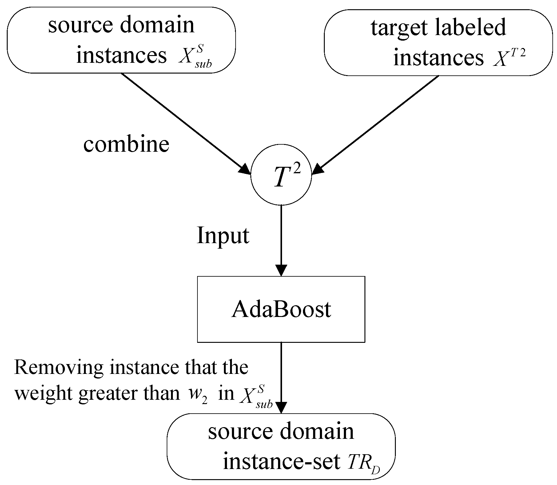
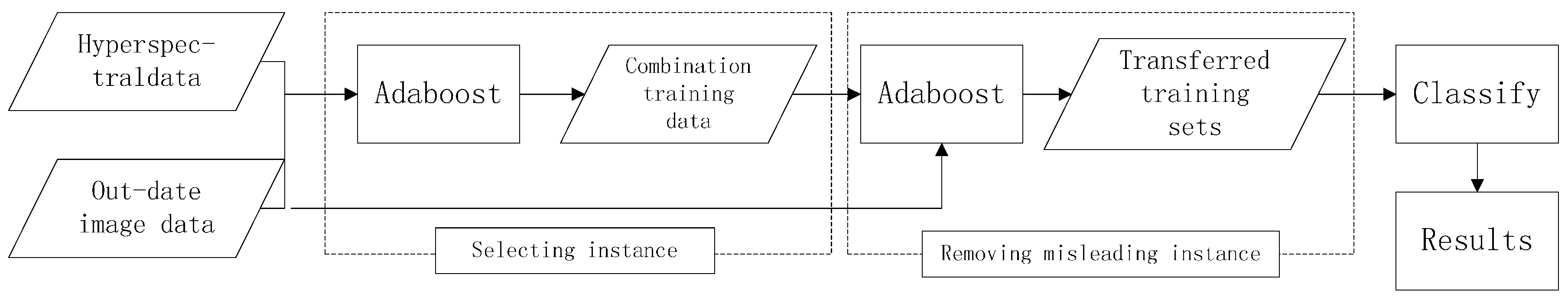
In this section, we provide empirical evidence that incorporating adaboost into the knowledge transfer framework results in better accuracies. We present results showing that the proposed method exhibits better learning rates than traditional classifiers with data points selected by only stacking. We also empirically show results that this method have a significant advantage in few training samples, comparing with the more traditional methods, by requiring fewer data points to obtain better classification accuracies.
In these experiments, SVM was used as the basic learners in transfer adaboost. SVM classification (adopting the LIBSVM library [
28]) was accomplished using a Gaussian RBF kernel. The SVM hyper parameters were optimized every ten iterations of the process by a fivefold cross validation. The C and
γ parameters were selected in the range [2
−5, 2
15] and [2
−15, 2
3], respectively. In the experiment, the network structure selected is regular network with 20 nodes and the degree is 10, the sampling parameter
ρ = 0.6, the training round
T = 10. Furthermore, some constraints were added to the basic learners to avoid the case of training weights being unbalanced. Thus, during training procedure, the overall training weights between positive and negative examples are consistently balanced.
Three benchmark methods are implemented by using SVM as shown in
Table 3. In the following, SVM, SVMt, TSVM will be used to represent various implementations of classifiers. SVMt means that training data will be only stacked by using SVM classifier. Moreover, the TSVM is the key method proposed in this paper.
The Botswana Hyperion data and ROSIS University of Pavia data set are respectively split into two sets: a training set
XS and a test set
S. We adopted KPCA algorithm to extract the image features including 30 dimensions [
29]. The comparison experiment based on TrAdaBoost is performed. In the experiment, the network structure selected is regular network with 20 nodes and the degree is 10, the sampling parameter
ρ = 0.6, the training round
T = 10.
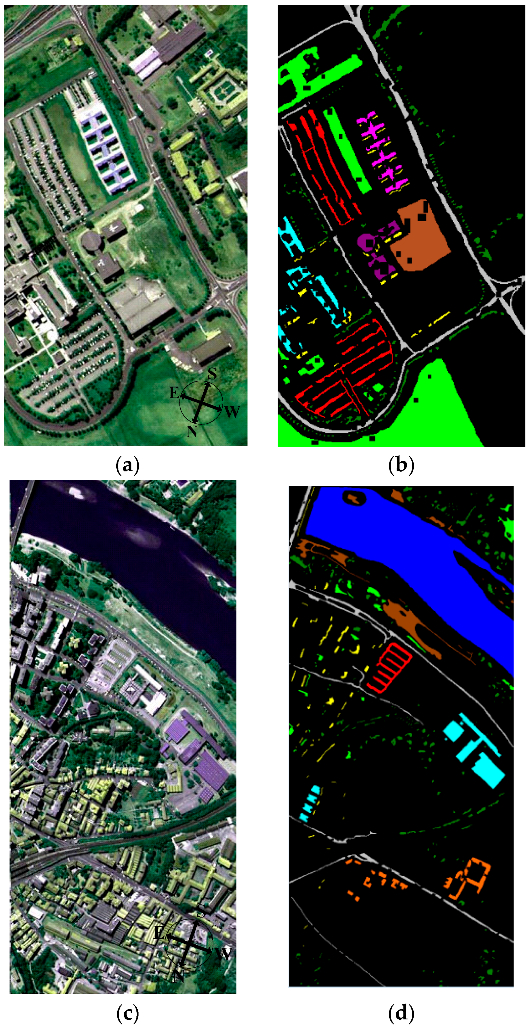
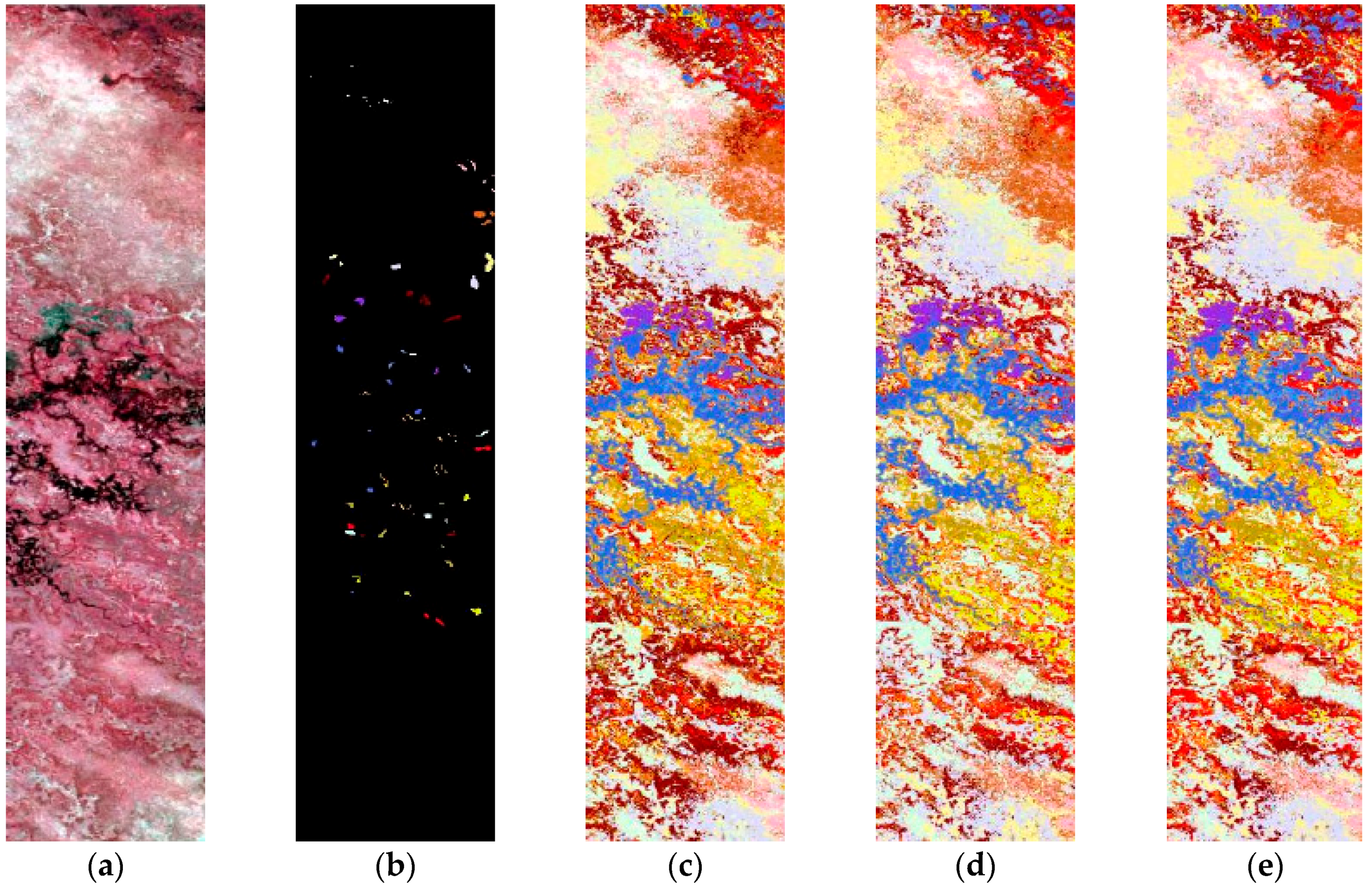
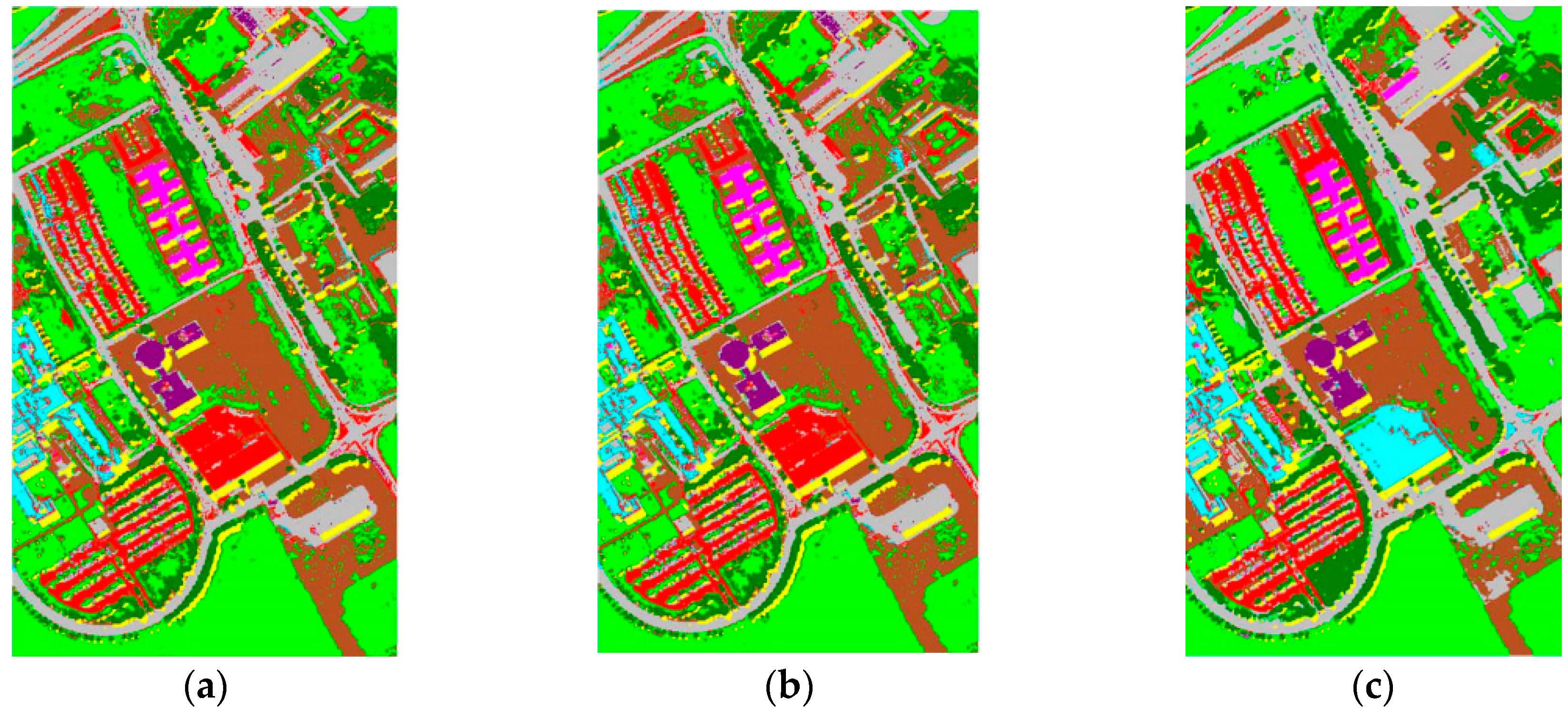
Table 4 presents the experimental results of SVM, SVMt and TrAdaBoost (TSVM) when the ratio between training and testing data is 2% and 5%. The performance in classification accuracy was the average of 10 repeats by random. Finally, the Botswana data classification maps obtained by the different methods are shown in
Figure 4 and the ROSIS data in
Figure 5.
From
Table 4, the accuracy given by TSVM are obviously higher than those given by SVM and SVMt. Intuitively, this is inevitable since SVM is not a learning technique designed for transfer classification, while adaboost is. However, as several researchers have already noted, transfer learning could not improve the generalization classification accuracy all the time and sometimes will show even lower performance on test set. This phenomenon is mentioned as transfer learning lowers the original performance negative transfer. Although in our experiments, adaboost continuously exhibit better or comparative performances than baselines, there is no guarantee for TrAdaboost to improve the basic learner.
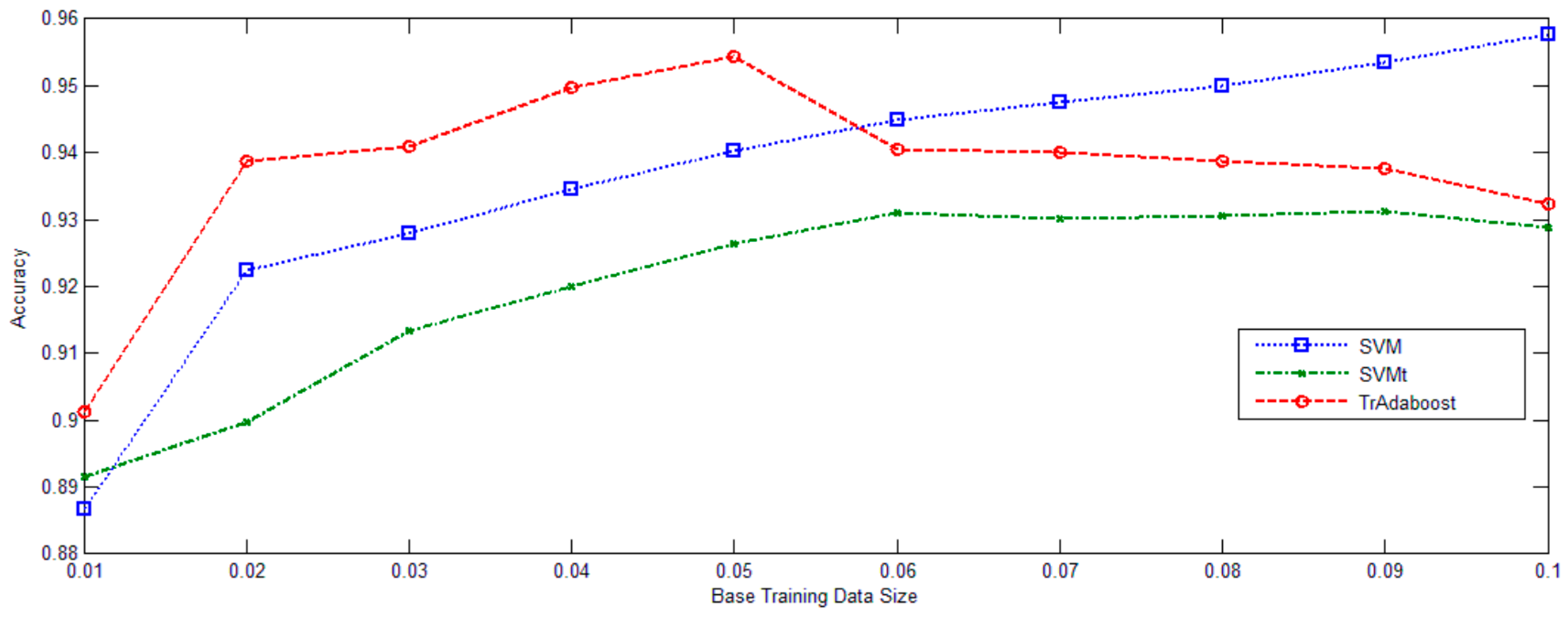
In
Figure 6, University of Pavia data set was deliberately used. The ratio between training and diff-distribution testing examples gradually increased from 0.01 to 0.1. Classifications were performed 10 times for each sampling rate. The average overall accuracies and standard deviations of the two baseline methods and the proposed method are listed in
Figure 5. TrAdaBoost (SVM) consistently improves the performance of SVMt. TrAdaBoost (SVM) also outperforms SVM, when the ratio is lower than 0.05. But, when the ratio reaches larger than 0.05, TrAdaBoost (SVM) performs a little worse than SVM, but still comparative. Generally out-date image set training data contain both good knowledge and noisy data. In the case of that too few original image set training data could be used to train a good classifier, the useful knowledge from out-date image set training data will be beneficial to the learner, while the noisy part does not have significant negative effect.
In the following discussion, ROSIS data were used as an illustrative example. This data set combination is representative of the remaining data sets as due to its similarity with some classes. We first use SVM classifier on the University of Pavia image data set. The resultant graph presents a misleading clustering condition, and consequently leads to an unfaithful joint manifold. Subsequently, as seen in the example in
Table 5, some misclassified samples are observed, e.g., for classes 2 and 4. It can be seen that the two classes, i.e., Meadow (Class 2) and Bare_soil (Class 4), exhibit significant confusion. Samples of Class 2 from the source image and samples of Class 4 from the target image are difficult to discriminate since the two features are very similar, which can also be validated by the confusion matrix in
Table 4. The separation of these two classes is clearer in the latent space provided by the proposed method. The same trend is observed for Classes 3 and 4 of the data, as well as these two class pairs of the Class 3 and Class 2. The Asphalt (Class 1) and Brick (Class 6) land cover types also show some confusion.
In addition to improvement of the classification accuracy, the proposed method also selects the most informative data points from these classes. Compared to the results given by the two baselines, TSVM provides higher overall accuracy. Among the ten common classes in the UOP data pair, classes 1, 2, 3, 4, 6 are difficult to discriminate within a single image because the classes are comprised of mixtures. Spectral changes and mixed spectral signatures make domain adaptation in these data pairs even more difficult. The Class 2/Class 4 pair exhibits the most confusion. As shown in
Figure 3, classes 2 and 4 from the source image (UOP) are very similar, and we can also observe that the spectral drifting of Class 2 is evident. Thus, many samples of Class 2 from the target image (COP) are misclassified as Class 4 when the training samples are only from the source image. The proposed method provides a significant improvement in the classification accuracy of Class 2.
Table 6 shows the confusion matrix obtained by using the TSVM algorithm. This method eliminates the confusion among some classes, and also exhibits a better accuracy in tree (Class 3), bare_soil (Class 4), bitumen (Class 5) and shadow (Class 7).


