
A Data Transfer Fusion Method for Discriminating Similar Spectral Classes


Abstract
:1. Introduction
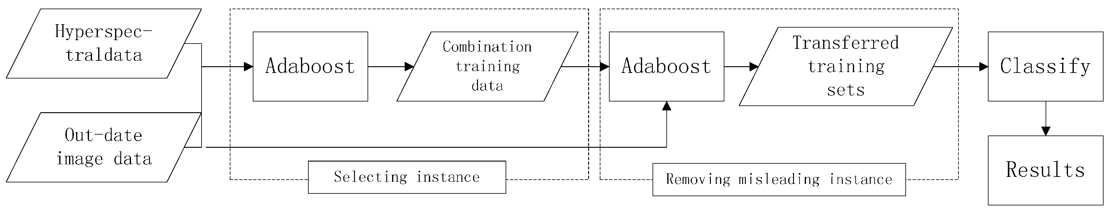
2. Transfer Learning Based Fusion Method
2.1. Selecting the Source Domain Instances to Append Labeled Target Domain Instances
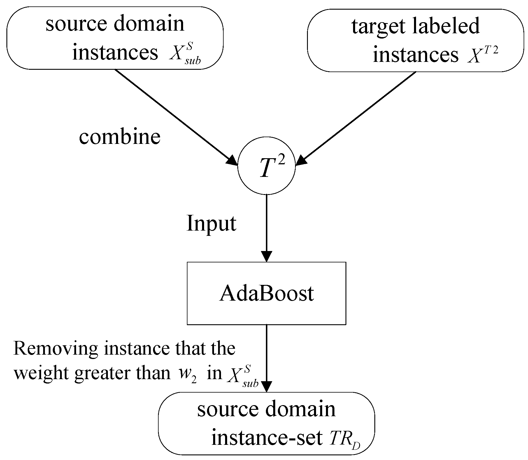
2.2. Removing “Misleading” Source Domain Instances
- Step 1.
- Generate a replicate training set of size , by weighted sub-sampling with replacement from training set and , k = 1, 2,…, K, respectively;
- Step 2.
- Train the classifier (node) in the classifiers network with respect to the weighted training set and obtain the hypothesis for multi-classification , k = 1, 2,…, K, where Y is the label set.
- Step 3.
- Calculate the weighted error rate of the instances in :
- Step 4.
- Hypothesize the classifier weight:
- Step 5.
- Set weights update parameters , and . Note that εk,t < 0.5.
- Step 6.
- Update the weight of instance i of node k:
3. Experiments and Discussion
3.1. Data Sets
3.1.1. Okavango Delta, Botswana
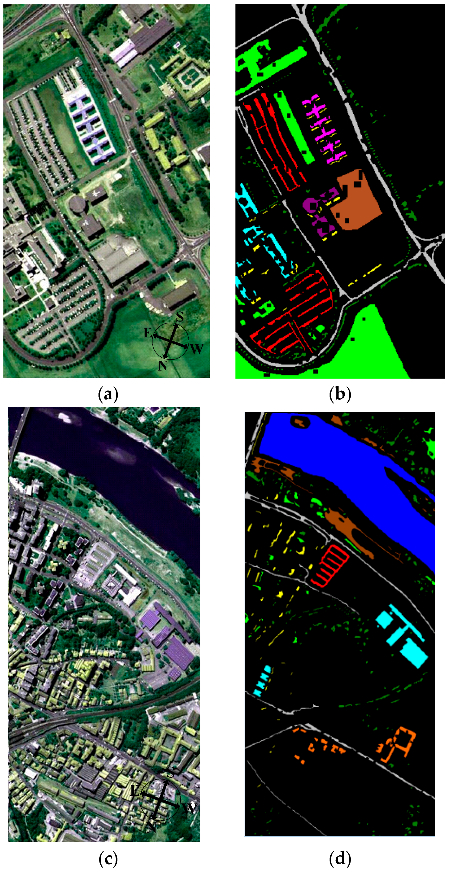
3.1.2. ROSIS Data
University Area
Pavia Center
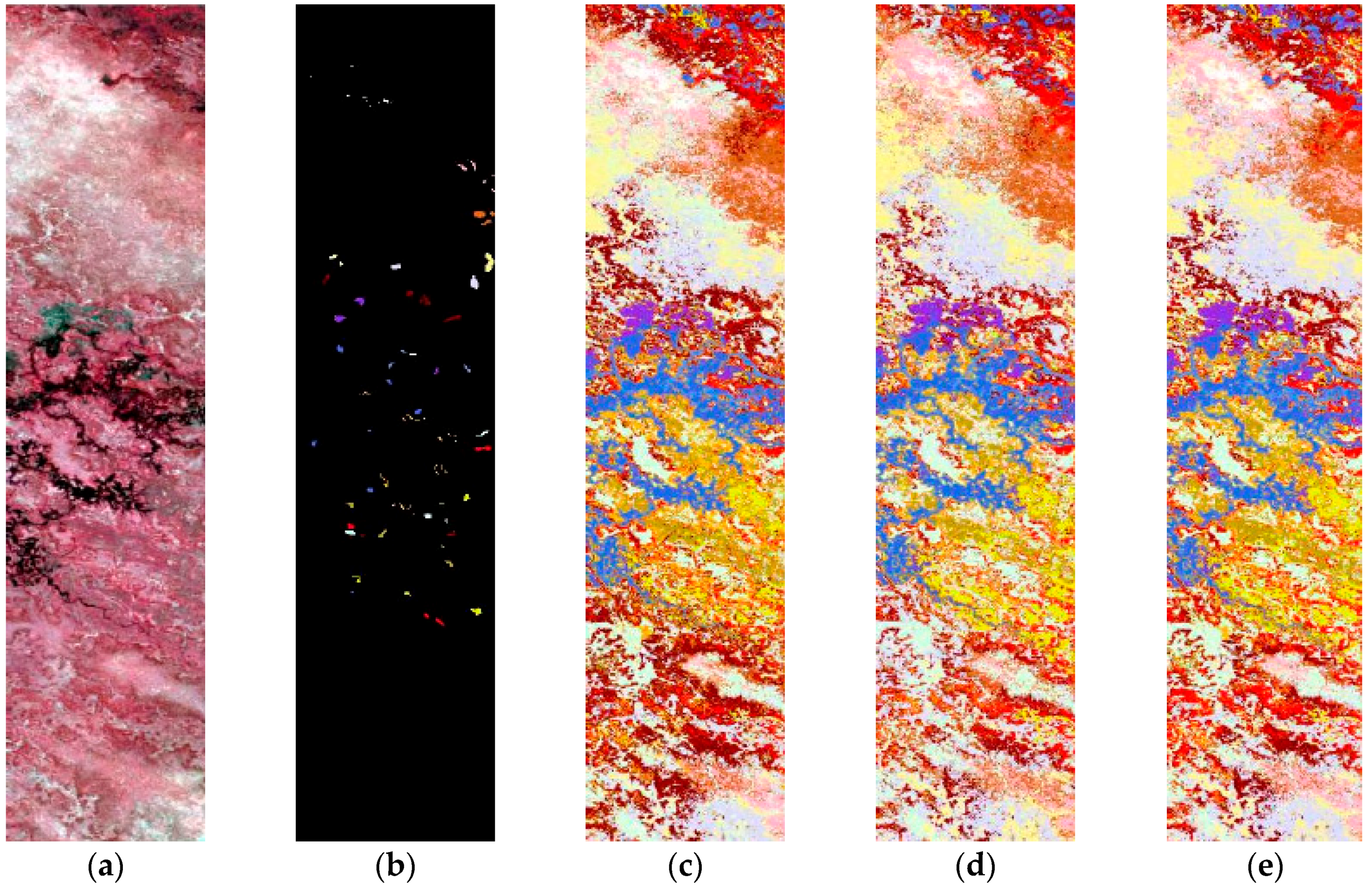
3.2. Experiments
4. Conclusions
Acknowledgments
Author Contributions
Conflicts of Interest
References
- Black, S.C.; Guo, X. Estimationof grassland CO2 exchange rates using hyperspectral remote sensing techniques. Int. J. Remote Sens. 2008, 29, 145–155. [Google Scholar] [CrossRef]
- Martin, M.E.; Smith, M.L.; Ollinger, S.V.; Plourde, L.; Hallett, R.A. The use of hyperspectral remote sensing in the assessment of forest ecosystem function. In Proceedings of the EPA Spectral Remote Sensing of Vegetation Conference, Las Vegas, NV, USA, 12–14 March 2003.
- Nidamanuri, R.R.; Garg, P.K.; Ghosh, S.K.; Dadhwal, V.K. Estimation of leaf total chlorophyll and nitrogen concentrations using hyperspectral satellite imagery. J. Agric. Sci. 2008, 146, 65–75. [Google Scholar]
- Zhang, Y.; Chen, J.M.; Miller, J.R.; Noland, T.L. Leaf chlorophyll content retrieval from airborne hyperspectral remote sensing imagery. Remote Sens. Environ. 2008, 112, 3234–3247. [Google Scholar] [CrossRef]
- Plaza, A.; Plaza, J.; Vegas, H. Improving the performance of hyperspectral image and signal processing algorithms using parallel, distributed and specialized hardware-based systems. J. Signal Process. Syst. 2010, 61, 293–315. [Google Scholar] [CrossRef]
- Fukunaga, K. Introduction to Statistical Pattern Recognition, 2nd ed.; Academic Press: New York, NY, USA, 1990. [Google Scholar]
- Chang, C.I. An information theoretic-based approach to spectral variability, similarity and discriminability for hyperspectral image analysis. IEEE Trans. Inf. Theory 2000, 46, 1927–1932. [Google Scholar] [CrossRef]
- Camps-Valls, G.; Bruzzone, L. Kernel-based methods for hyperspectral image classification. IEEE Trans. Geosci. Remote Sens. 2005, 43, 1351–1362. [Google Scholar] [CrossRef]
- Demir, B.; Erturk, S. Hyperspectral image classification using relevance vector machines. IEEE Geosci. Remote Sens. Lett. 2007, 4, 586–590. [Google Scholar] [CrossRef]
- Sun, Z.; Wang, C.; Wang, H.; Li, J. Learn multiple-kernel SVMs for domain adaptation in hyperspectral data. IEEE Geosci. Remote Sens. Lett. 2013, 10, 1224–1228. [Google Scholar]
- Crawford, M.M.; Ma, L.; Kim, W. Exploring nonlinear manifold learning for classification of hyperspectral data. In Optical Remote Sensing; Springer: New York, NY, USA, 2011; pp. 207–234. [Google Scholar]
- Li, W.; Prasad, S. Locality-preserving dimensionality reduction and classification for hyperspectral image analysis. IEEE Trans. Geosci. Remote Sens. 2012, 50, 1185–1198. [Google Scholar] [CrossRef]
- Zhang, L.; Zhang, L.; Tao, D.; Huang, X. On combining multiple features for hyperspectral remote sensing image classification. IEEE Trans. Geosci. Remote Sens. 2012, 50, 879–893. [Google Scholar] [CrossRef]
- Pan, S.J.; Yang, Q. A survey on transfer learning. IEEE Trans. Knowl. Data Eng. 2010, 22, 1345–1359. [Google Scholar] [CrossRef]
- Dai, W.Y.; Yang, Q. Boosting for Transfer Learning. In Proceedings of the 24th Annual International Conference on Machine Learning, Corvallis, OR, USA, 20–24 June 2007; pp. 193–200.
- Jiang, J.; Zhai, C. Instance weighting for domain adaptation in NLP. In Proceedings of the 45th Annual Meeting of the Association for Computational Linguistics, Prague, Czech Republic, 24–29 June 2007; pp. 264–271.
- Wang, C.; Mahadevan, S. Heterogeneous domain adaptation using manifold alignment. In Proceedings of the 22nd International Joint Conference on Artificial Intelligence, Barcelona, Spain, 16–22 July 2011; pp. 1541–1546.
- Lafon, S.; Keller, Y.; Coifman, R.R. Data fusion and multicue data matching by diffusion maps. IEEE Trans. Pattern Anal. 2006, 28, 1784–1797. [Google Scholar] [CrossRef] [PubMed]
- Ham, J.; Lee, D.D.; Saul, L.K. Semisupervised alignment of manifolds. In Proceedings of the Tenth International Workshop on Artificial Intelligence and Statistics, Bridgetown, Barbados, 6–8 January 2005; pp. 120–127.
- Bue, B.D.; Merenyi, E. Using spatial correspondences for hyperspectral knowledge transfer: Evaluation on synthetic data. In Proceedings of the 2nd Workshop on Hyperspectral Image and Signal Processing: Evolution in Remote Sensing (WHISPERS), Reykjavik, Iceland, 14–16 June 2010; pp. 14–16.
- Knorn, J.; Rabe, A.; Radeloff, V.C.; Kuemmerle, T.; Kozak, J.; Hostert, P. Land cover mapping of large areas using chain classification of neighboring Landsat satellite images. Remote Sens. Environ. 2009, 113, 957–964. [Google Scholar] [CrossRef]
- Liu, Y.; Cheng, J.; Xu, C.; Lu, H. Building topographic subspace model with transfer learning for sparse representation. Neurocomputing 2010, 73, 1662–1668. [Google Scholar] [CrossRef]
- Yang, H.L.; Crawford, M.M. Learning a joint manifold with global-local preservation for multitemporal hyperspectral image classification. In Proceedings of the IEEE International Geoscience and Remote Sensing Symposium (IGARSS), Melbourne, Australia, 21–26 July 2013; pp. 21–26.
- Persello, C.; Bruzzone, L. Kernel-based domain-invariant feature selection in hyperspectral images for transfer learning. IEEE Trans. Geosci. Remote Sens. 2015, 99, 1–9. [Google Scholar] [CrossRef]
- Yang, H.L.; Crawford, M.M. Domain Adaptation with preservation of manifold geometry for hyperspectral image classification. IEEE J. Sel. Top. Appl. Earth Obs. Remote Sens. 2016, 9, 543–555. [Google Scholar] [CrossRef]
- Ham, J.S.; Chen, Y.C.; Crawford, M.M.; Ghosh, J.G. Investigation of the random forest framework for classification of hyperspectral data. IEEE Trans. Geosci. Remote Sens. 2005, 43, 492–501. [Google Scholar] [CrossRef]
- Zhang, Z.; Pasolli, E.; Crawford, M.M.; Tilton, J.C. An active learning framework for hyperspectral image classification using hierarchical segmentation. IEEE J. Sel. Top. Appl. Earth Obs. Remote Sens. 2016, 9, 640–654. [Google Scholar]
- Chang, C.; Lin, C. LIBSVM—A Library for Support. Vector Machine. 2008. Available online: http://www.csie.ntu.edu.tw/~cjlin/libsvm (accessed on 10 November 2015).
- Gu, Y.F.; Liu, Y.; Zhang, Y. A selective KPCA algorithm based on high-order statistics for anomaly detection in hyperspectral imagery. IEEE Geosci. Remote Sens. Lett. 2008, 5, 43–47. [Google Scholar]


| No. | Class Name | Area 1 | Area 2 |
|---|---|---|---|
| 1 | Water | 270 | 126 |
| 2 | Hippo grass | 101 | 162 |
| 3 | Floodplain grasses1 | 251 | 158 |
| 4 | Floodplain grasses2 | 215 | 165 |
| 5 | Reeds1 | 269 | 168 |
| 6 | Riparian | 269 | 211 |
| 7 | Firescar2 | 259 | 176 |
| 8 | Island interior | 203 | 154 |
| 9 | Acacia woodlands | 314 | 151 |
| 10 | Acacia shrublands | 248 | 190 |
| 11 | Acacia grasslands | 305 | 358 |
| 12 | Short mopane | 181 | 153 |
| 13 | Mixed mopane | 268 | 233 |
| 14 | Exposed soils | 95 | 89 |
| No. | Center of Pavia | University of Pavia | COP | UOP |
|---|---|---|---|---|
| 1 | Asphalt | Asphalt | 9248 | 6641 |
| 2 | Meadow | Meadow | 3090 | 18,649 |
| 3 | Tree | Tree | 7598 | 3064 |
| 4 | Bare_soil | Bare_soil | 6584 | 5029 |
| 5 | Bitumen | Bitumen | 7287 | 1330 |
| 6 | Brick | Brick | 2685 | 3682 |
| 7 | Shadow | Shadow | 2863 | 945 |
| 8 | Tile | Gravel | 42,826 | 2099 |
| 9 | Water | Metal_sheet | 65,971 | 1345 |
| Benchmark | Training Data | Test Data | Basic Learner | |
|---|---|---|---|---|
| Labeled | Unlabeled | |||
| SVM |  |  | S | SVM |
| SVMt |  |  | S | SVM |
| TSVM |  | S | S | SVM |
| Ratio | Botswana | UOP | ||||
|---|---|---|---|---|---|---|
| SVM | SVMt | TSVM | SVM | SVMt | TSVM | |
| 2% | 0.9013 | 0.8832 | 0.9105 | 0.9225 | 0.8952 | 0.9387 |
| 5% | 0.9171 | 0.9053 | 0.9210 | 0.9449 | 0.9265 | 0.9543 |
| Ground Truth (Pixels) | |||||||||
|---|---|---|---|---|---|---|---|---|---|
| Class | Asphlt | Meadow | Tree | Bare_Soil | Bitumen | Brick | Shadow | ||
| Classified image (pixels) | Asphalt | 5953 | 19 | 1 | 23 | 303 | 205 | 6 | |
| Meadow | 0 | 17,118 | 126 | 500 | 0 | 8 | 0 | ||
| Tree | 14 | 272 | 2937 | 40 | 0 | 2 | 0 | ||
| Bare_soil | 28 | 895 | 15 | 3867 | 0 | 44 | 0 | ||
| Bitumen | 218 | 0 | 0 | 0 | 1071 | 0 | 0 | ||
| Brick | 159 | 24 | 1 | 17 | 6 | 3476 | 2 | ||
| Shadow | 61 | 0 | 0 | 2 | 0 | 0 | 912 | ||
| Accuracy | 89.10 | 93.96 | 87.65 | 77.70 | 80.95 | 91.91 | 91.11 | 92.25 | |
| Ground Truth (Pixels) | |||||||||
|---|---|---|---|---|---|---|---|---|---|
| Class | Asphalt | Meadow | Tree | Bare_Soil | Bitumen | Brick | Shadow | ||
| Classified image (pixels) | Asphalt | 5762 | 13 | 1 | 34 | 395 | 301 | 4 | |
| Meadow | 3 | 16,546 | 193 | 601 | 0 | 6 | 0 | ||
| Tree | 14 | 207 | 3015 | 24 | 1 | 4 | 0 | ||
| Bare_soil | 17 | 526 | 12 | 4230 | 0 | 64 | 0 | ||
| Bitumen | 205 | 0 | 0 | 0 | 1080 | 4 | 0 | ||
| Brick | 129 | 33 | 0 | 61 | 58 | 3388 | 0 | ||
| Shadow | 25 | 0 | 1 | 0 | 0 | 0 | 949 | ||
| Accuracy | 88.57 | 93.21 | 89.82 | 85.07 | 83.69 | 89.49 | 95.41 | 93.87 | |
© 2016 by the authors; licensee MDPI, Basel, Switzerland. This article is an open access article distributed under the terms and conditions of the Creative Commons Attribution (CC-BY) license (http://creativecommons.org/licenses/by/4.0/).
Share and Cite
Wang, Q.; Zhang, J. A Data Transfer Fusion Method for Discriminating Similar Spectral Classes. Sensors 2016, 16, 1895. https://doi.org/10.3390/s16111895
Wang Q, Zhang J. A Data Transfer Fusion Method for Discriminating Similar Spectral Classes. Sensors. 2016; 16(11):1895. https://doi.org/10.3390/s16111895
Chicago/Turabian StyleWang, Qingyan, and Junping Zhang. 2016. "A Data Transfer Fusion Method for Discriminating Similar Spectral Classes" Sensors 16, no. 11: 1895. https://doi.org/10.3390/s16111895
APA StyleWang, Q., & Zhang, J. (2016). A Data Transfer Fusion Method for Discriminating Similar Spectral Classes. Sensors, 16(11), 1895. https://doi.org/10.3390/s16111895