1. Introduction
Chinese liquors are well-known beverages all over the world. The consumed amount and value in 2014 were reported to be 75,282.7 million liters and $133.25 billion United States Dollars (USD) [
1]. The enticing flavor profile for which Chinese liquors are so renowned is the result of the metabolic activity of a microbial community which provides thousands of micro-constituents such as esters, acids, phenols, and carbonyl compounds, etc. Chinese liquors are classified into 12 different flavors according to the content and type of the microconstituents [
2]. The analysis of the aroma of Chinese liquors is an especially complex problem due to the components’ complexity and similarity. The traditional method of the analysis and identification of Chinese liquors is by professional sommeliers [
3], but their accuracy and objectivity cannot be always ensured because sommeliers are affected by health conditions, emotions and the environment. Chromatographic [
4] and spectroscopic [
5] chemical analysis methods have been used to measure Chinese liquor products. However, these chemical analysis methods need to use large-scale devices and consume a lot of time, which could cause inevitable inconveniences for users. Taste sensors [
6], systems composed of a sensor array and a data-processing unit, based on several transduction mechanisms such as voltammetry [
7,
8], conductivity [
9] and potentiometry [
10,
11], can be used to identify liquid media containing multiple taste components. Detection equipment based on taste sensors could also be used to identify Chinese liquors, but the high cost of the equipment limits their broad application. The development of odor, vapor, and gas detection systems comprised of multi-sensor arrays together with pattern recognition techniques constituting so-called electronic nose systems is a fledgling area with applications in a variety of detection and identification problems [
12]. Electronic nose systems have been used in the food industry for the inspection of food quality [
13], control of cooking processes [
14], and food flavor assessment [
15], e.g., due to their objectivity, portability, accuracy, low cost and shorter analysis time.
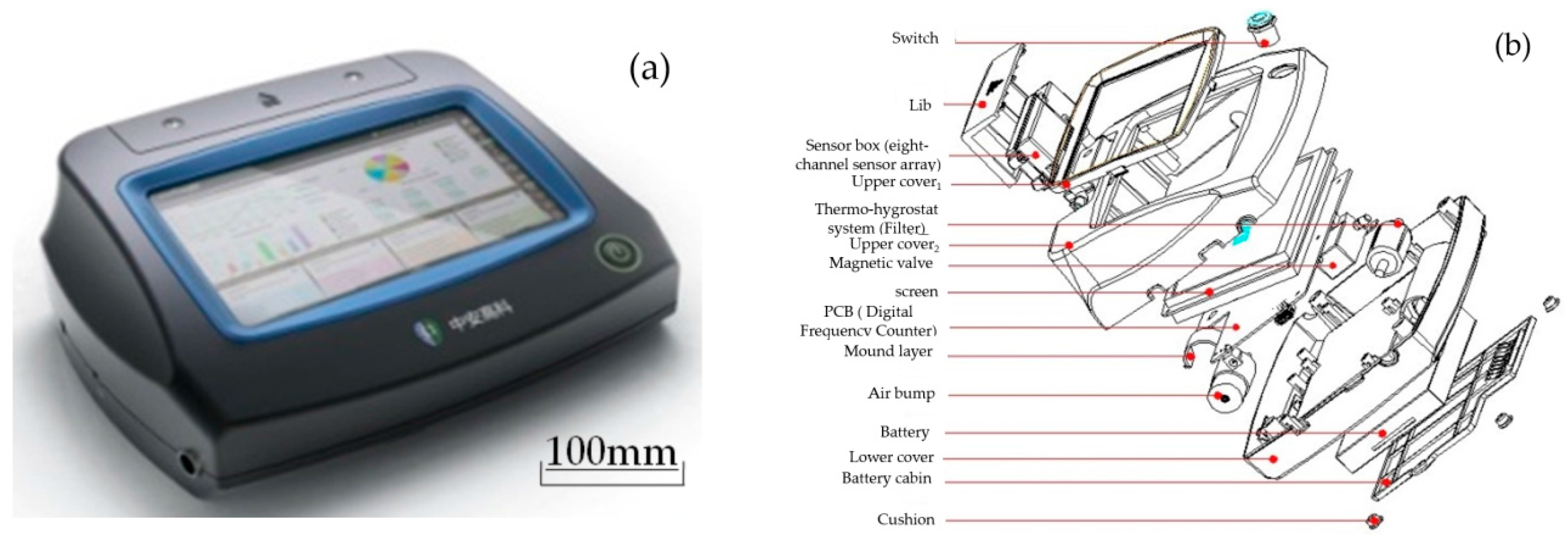
Our group has reported the design and application of a novel polymer piezoelectric sensor electronic nose (e-nose) [
16]. The e-nose is used for quickly and easily summarizing Chinese liquor flavor characteristics and provides an objective method of communication between engineers and end-users. The e-nose is an instrument consisting of an array of reversible but only semi-selective gas sensors coupled with a series of pattern recognition algorithms. Gu et al. [
17,
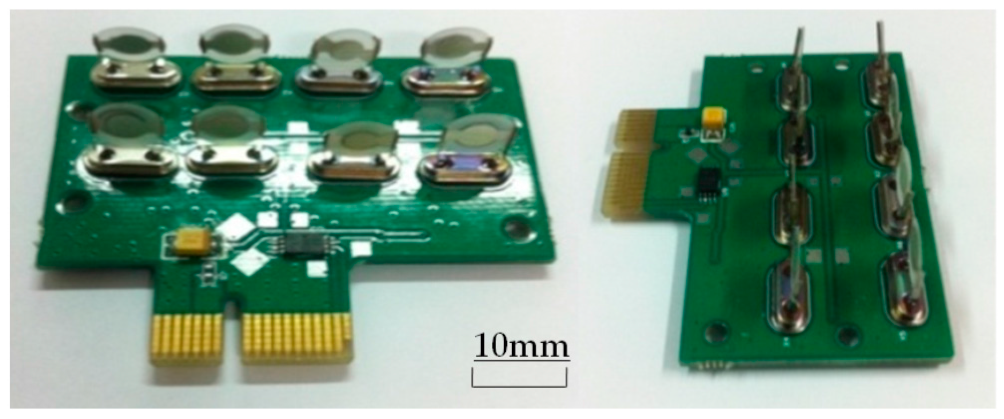
18] used the e-nose to classify different kinds of Chinese liquors by developing two pattern recognition systems based on linear discriminant analysis (LDA), and a back propagation (BP) neutral network method. The identification accuracies of LDA, and BP in predicting outcomes were 93.3% and 98%, respectively. To improve the identification accuracy of the e-nose, these methods should be conducted not only by developing a pattern recognition system, but also capturing the raw data (the testing frequency values) accurately. Semi-selective gas sensors that incorporate two polymer detection layers and transform an interaction into a testing frequency signal are used as transducers [
19]. The testing frequency values, the resonance frequency values of each sensor at stable state, are implemented to distinguish Chinese liquors [
17]. Those frequency values decrease at first and then stabilize in the adsorption phase, corresponding to the quartz crystal microbalance (QCM) principle [
16]. However, the principle fails to completely account for a particular phenomenon—we found that the resonance frequency values fluctuated in the stable state. The resonance frequency values fluctuations are caused by small amplitudes of buffeting of each sensor, the structure of which is seen as a thin flat plate, due to flow-induced forces. The study of the flow around the above plate-like structures is of great practical interest for improving the accuracy of the detection equipment.
Much theoretical and experimental effort has been expended to study the aerodynamic response of the plates and characterize the aerodynamic forces exerted on the plates. Wang and Eldredge [
20] established a low-order point vortex model to investigate vortex shedding from both the trailing and leading edges of a flat plate and to predict un-steady aerodynamic forces on the plate. Fedoul et al. [
21] conducted a wind tunnel experiment for the flow around a single flat plate and an array of three parallel flat plates at different angles of incidence. Their results indicated that the aerodynamic coefficient in an array of three parallel flat plates is shown to be larger than that obtained with an isolated plate only when the aspect ratio is large enough. Lin et al. [
22] considered the instantaneous angle of attack for obtaining aerodynamic forces on a thin flat plate of large oscillation amplitude. They concluded that the forced torsional and vertical oscillations of large amplitude have nonlinear influence on the aerodynamic force coefficients. Bruno et al. [
23] proposed an efficient method to deal with the characterization of the aerodynamic and aeroelastic behavior of a flat plate under uncertain flow conditions, and several examples of different representations of the stochastic outputs are given. Legresley et al. [
24] researched the probabilistic response of a nonlinear panel in supersonic flow. They found that the panel’s response is much more sensitive to the location of the modulus fields’ extrema values than their correlation length. Poirel et al. [
25] performed numerical studies for obtaining the flutter mechanism of a flexibly mounted rigid flat plate. Their results showed that the longitudinal component of turbulence lowers the flutter speed. It is believed that the decrease in flutter speed is mainly due to the small frequencies of the turbulence excitation.
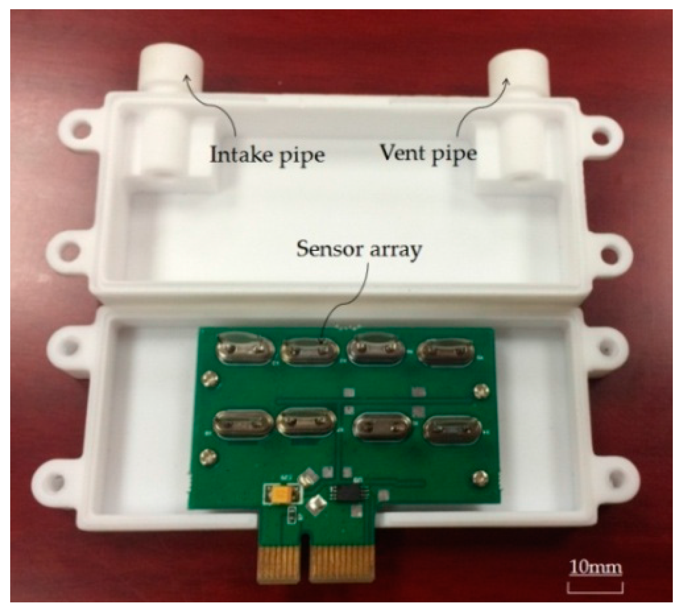
For the e-nose we employed, the sensor array containing the eight sensors is fixed in a sensor box. The geometric construction of the sensor box is quite simple, but the physics describing the flow inside the box are very complex due to the three dimensional nature of flow and the interactions between the gas flow, the sensors and the sensor box’s cavity. The exact nature of gas flow inside the sensor box and the flow-induced forces on the sensors are not yet completely understood. In this paper, the realistic gas flow in the sensor box was studied utilizing CFD tools, enabling a full 3D analysis of the aerodynamic effect of the sensors on the impact of volatile gas of Chinese liquors. The aerodynamic characteristics of the eight sensors are presented and the influence on the resonance frequency values fluctuations by the flow-induced forces is evaluated. In this paper, we also employed the following nomenclature, as listed in
Table 1.
3. Assumption Define and Geometric Model
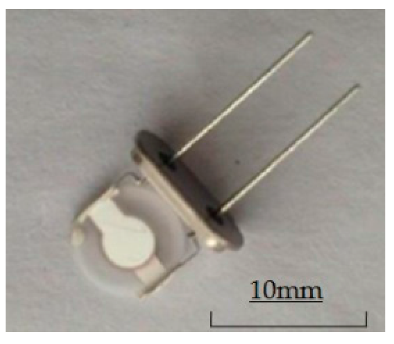
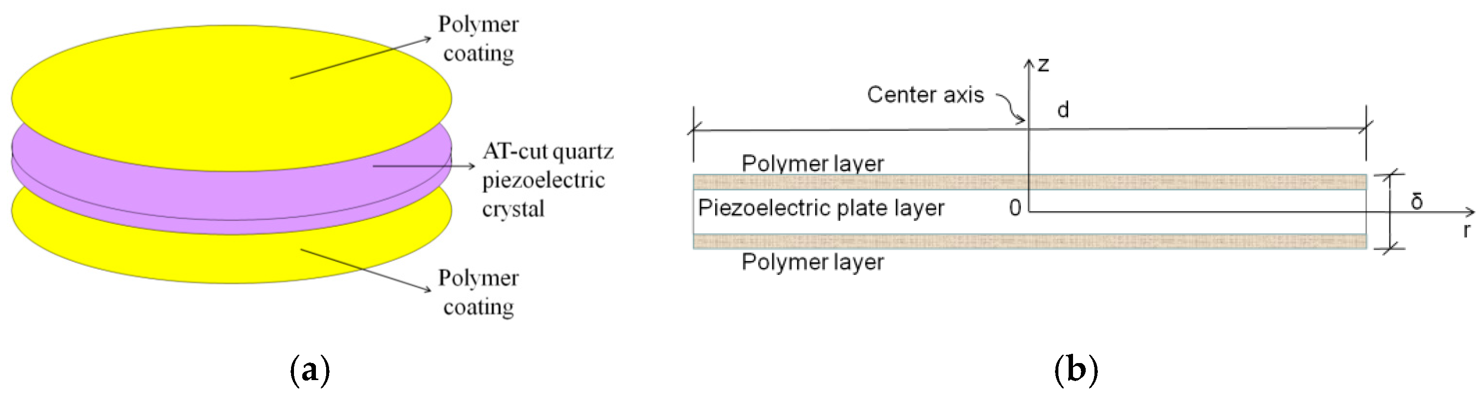
This study focuses on flow-induced forces on the sensors. The natural oscillations are high resonance frequency values from 9.991743 MHz to 9.997071 MHz. In order to model the aerodynamic forces problem, several assumptions are made here in advance. First of all, the sensor's oscillatory vibration motion is neglected; this is justifiable as a first approximation since the vibration amplitude of each sensor is relatively small at high frequencies. Then, under the above simplification, the inertia forces inherent in the sensor’s oscillatory vibration motion were not taken into account. Finally, we assume that the thickness of the sensors is negligible due to the diameter-to-thickness ratio (d/δ) of each sensor being 47 (
Figure 5).
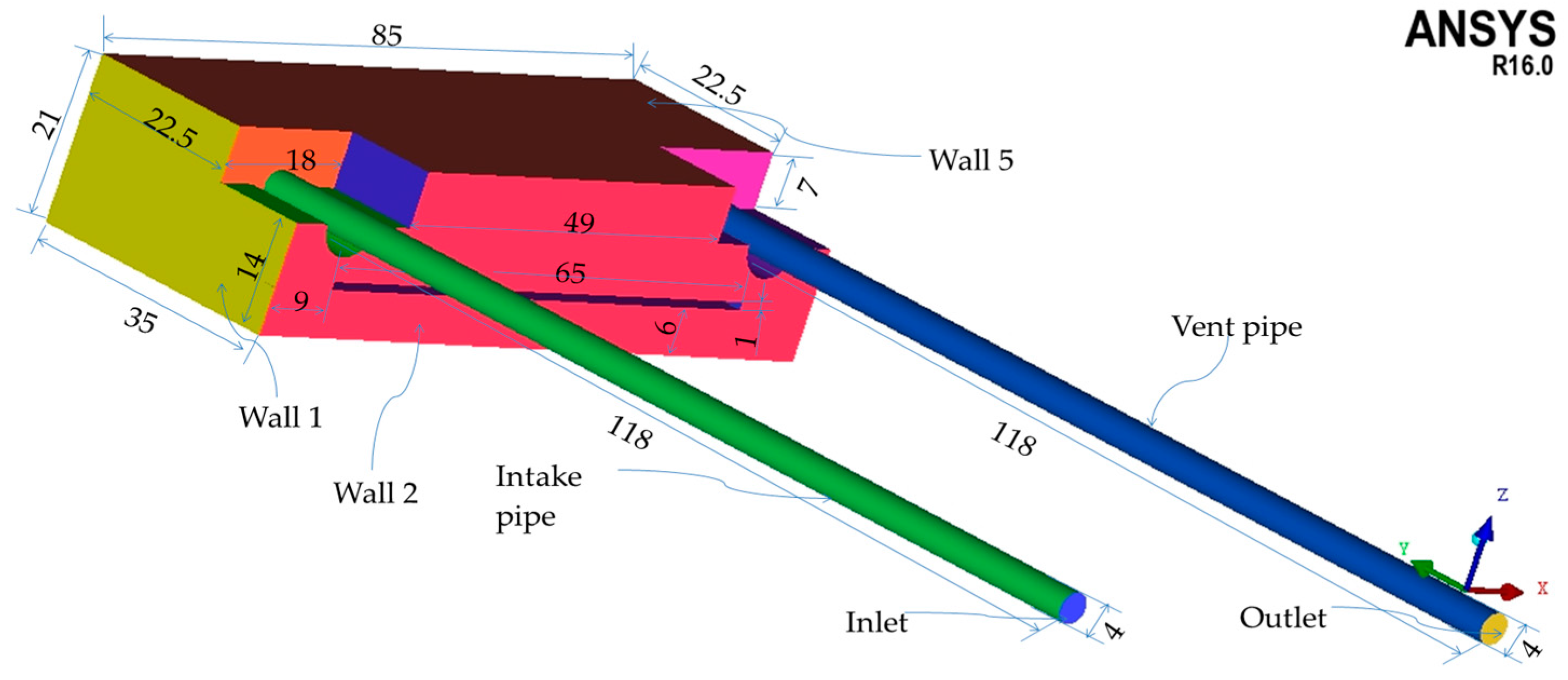
To represent simply but realistically the geometry of the sensor box, a dedicated procedure was conducted for the reconstruction of the 3D sensor box model from the available database.
Figure 8 shows the dimensions of sensor box's cavity from a global-view image.
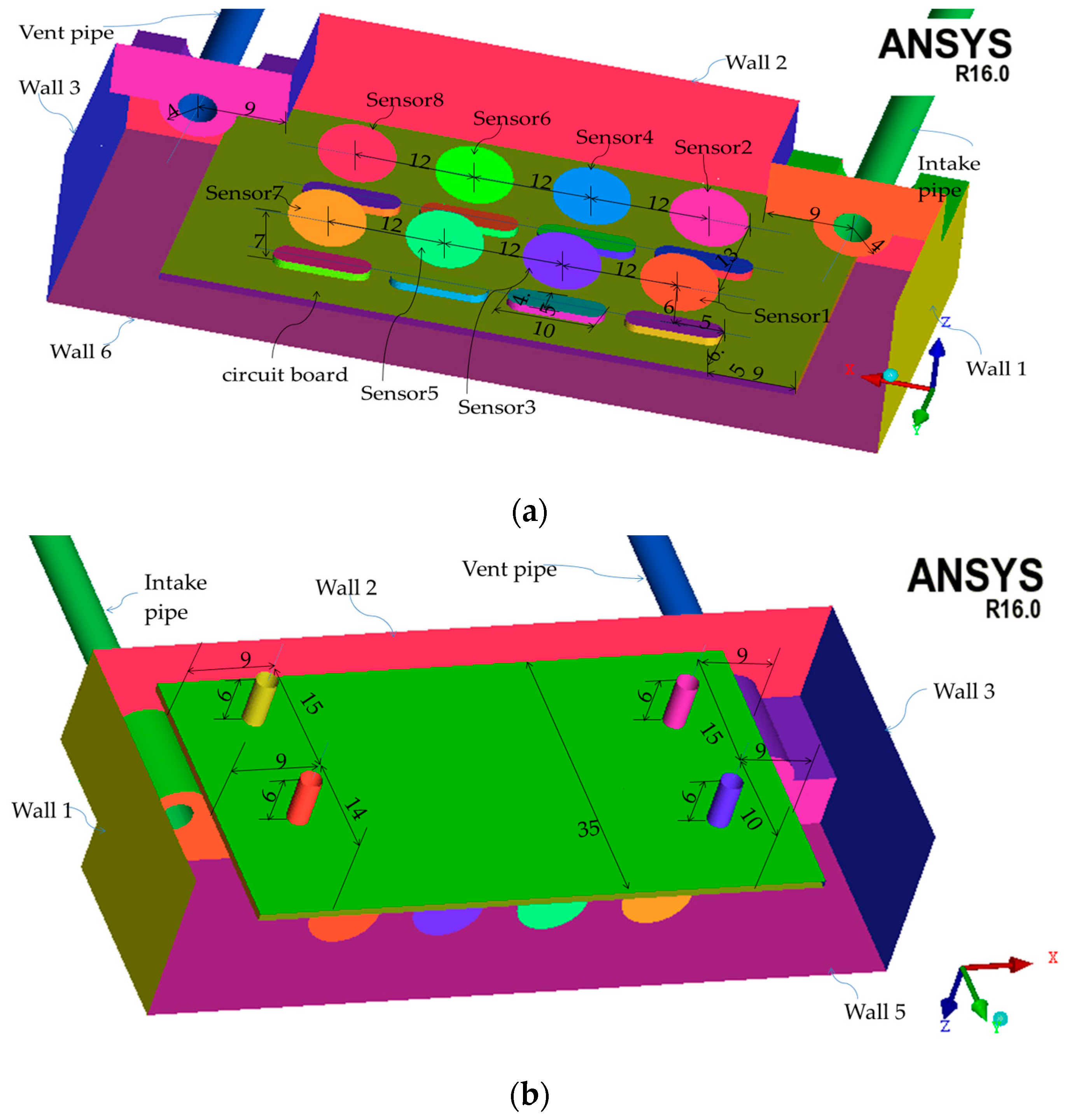
Figure 9 also shows the global coordinates of the sensor box model. The global coordinates have x axis normal to the “Wall 1”, y axis perpendicular to the “Wall 2”, and z axis normal to the “Wall 5”. The origin of global coordinates is fixed at the point “o”.
Figure 9a,b display the dimensions of the structures in sensor box’s cavity from two partial-view images. “Wall 4” is not presented in either of
Figure 8a,b in order to display the structures clearly.
The principal components of the
Maotai are water and alcohol. The determining factor of the
Maotai flavor are the complex trace organic compounds present in this Chinese liquor, such as ethyl palmitate [
29]. In order to reduce the indispensable computation process for further modeling, the volatile gas of
Maotai, the volatile gas of Chinese liquor, could be assumed as a mixture of gases containing 53% (mole fraction) alcohol vapor, 46.5% (mole fraction) water vapor and 0.5% (mole fraction) ethyl palmitate (C
18H
36O
2) gas.
4. Modeling
4.1. Governing Equations in Scenario
The governing equations are the conservations of mass, momentum, energy and species diffusion, are as follows:
Also, assuming that the variations of temperature across the sensor box are negligible, the mixture density is calculated based on the ideal mixture state [
30] at the working temperature and pressure:
Other thermo-physical properties of the mixture such as constant-pressure specific heat, thermal conductivity, and dynamic viscosity are calculated based on the mixture composition, as stated in [
30,
31].
4.2. CFD Approach
The governing equations of the gas flow in sensor box were discretized by means of the finite volume method. The discretized algebraic equations were solved iteratively by using the unstructured CFD solver, Fluent 16.0 (ANSYS, Pittsburgh, PA, USA). The software ICEM (ANSYS, Pittsburgh, PA, USA) was used as a preprocessing tool of Fluent for mesh generation.
4.3. Mesh Generation
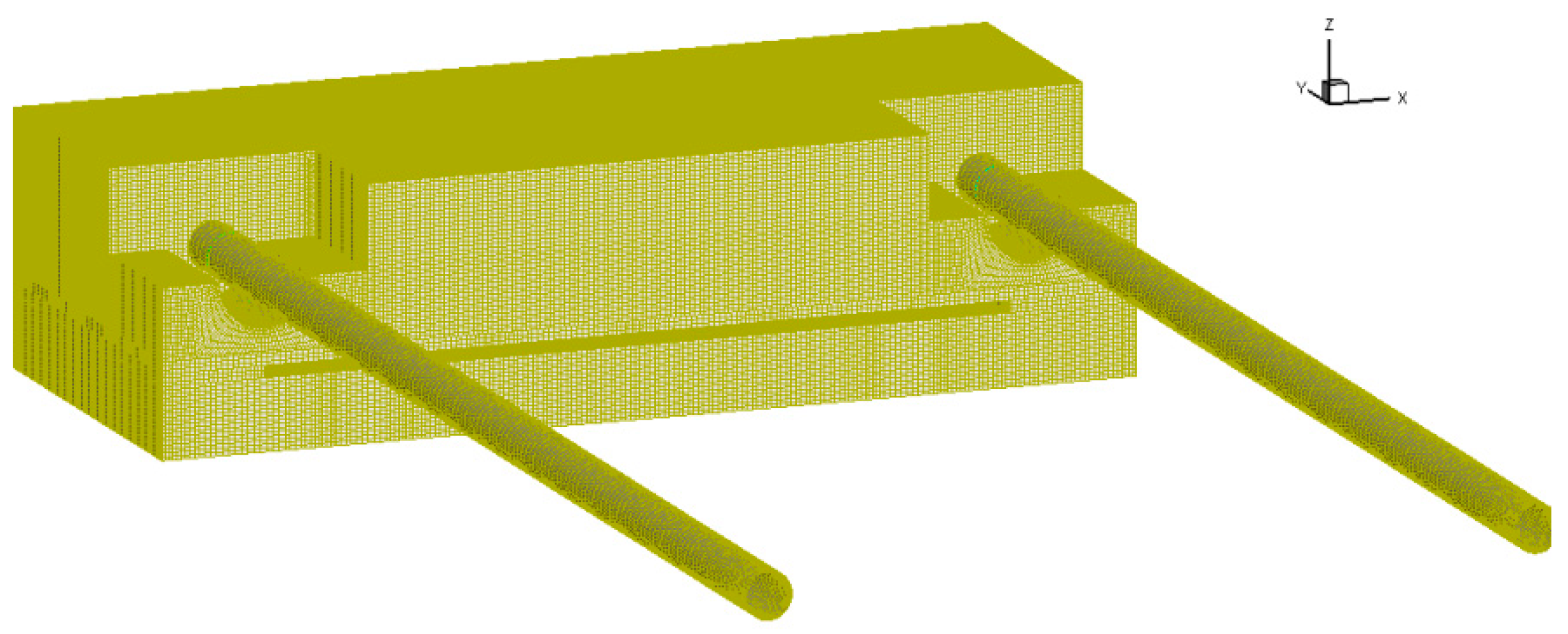
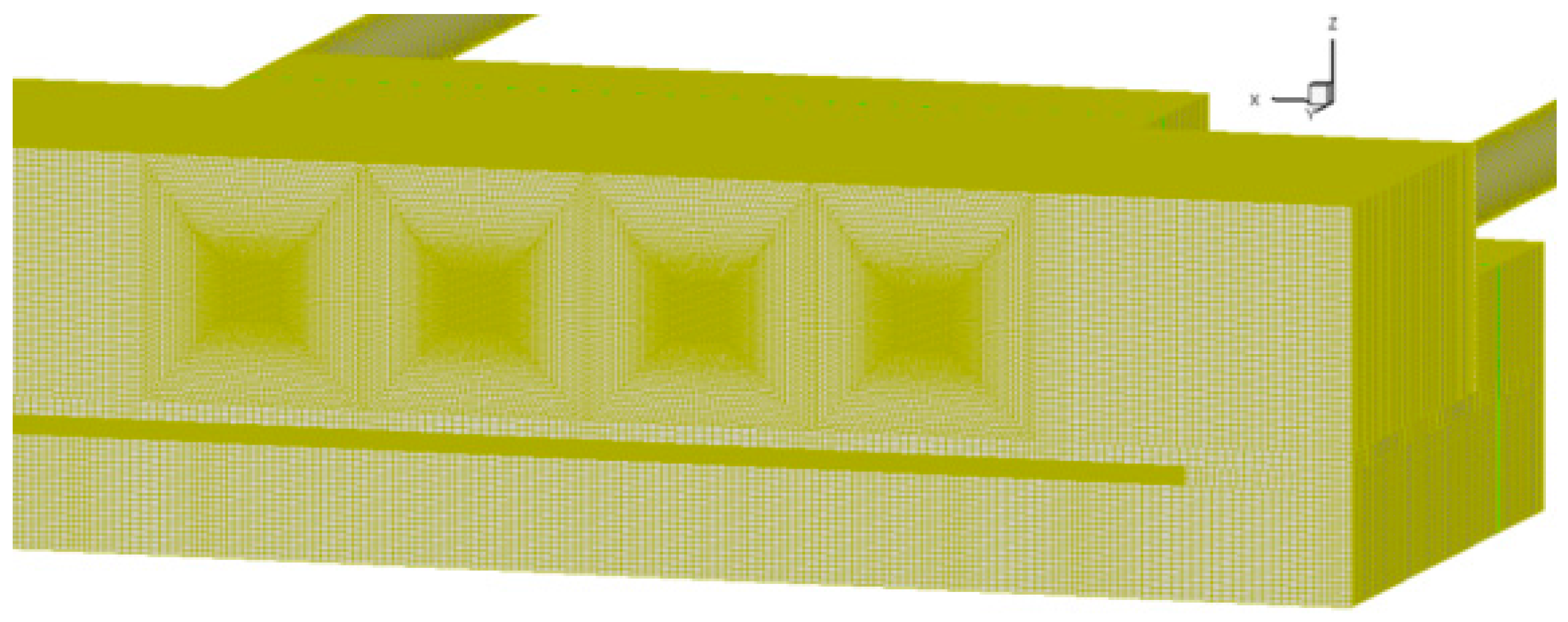
The mesh of the computational domain generated by ICEM was shown in
Figure 10. A partial-view image of the mesh could be seen in
Figure 10. The sensor box’s cavity was decomposed into seven blocks so as to generate a fine structural hexahedral mesh. The generated mesh had maximum density near each sensor, which decreases smoothly towards the wall of the cavity. The mesh design of 2,529,639 nodes was chosen for evaluation of flow-induced forces on each sensor after performing steady simulation for a grid independence study.
4.4. Boundary Conditions
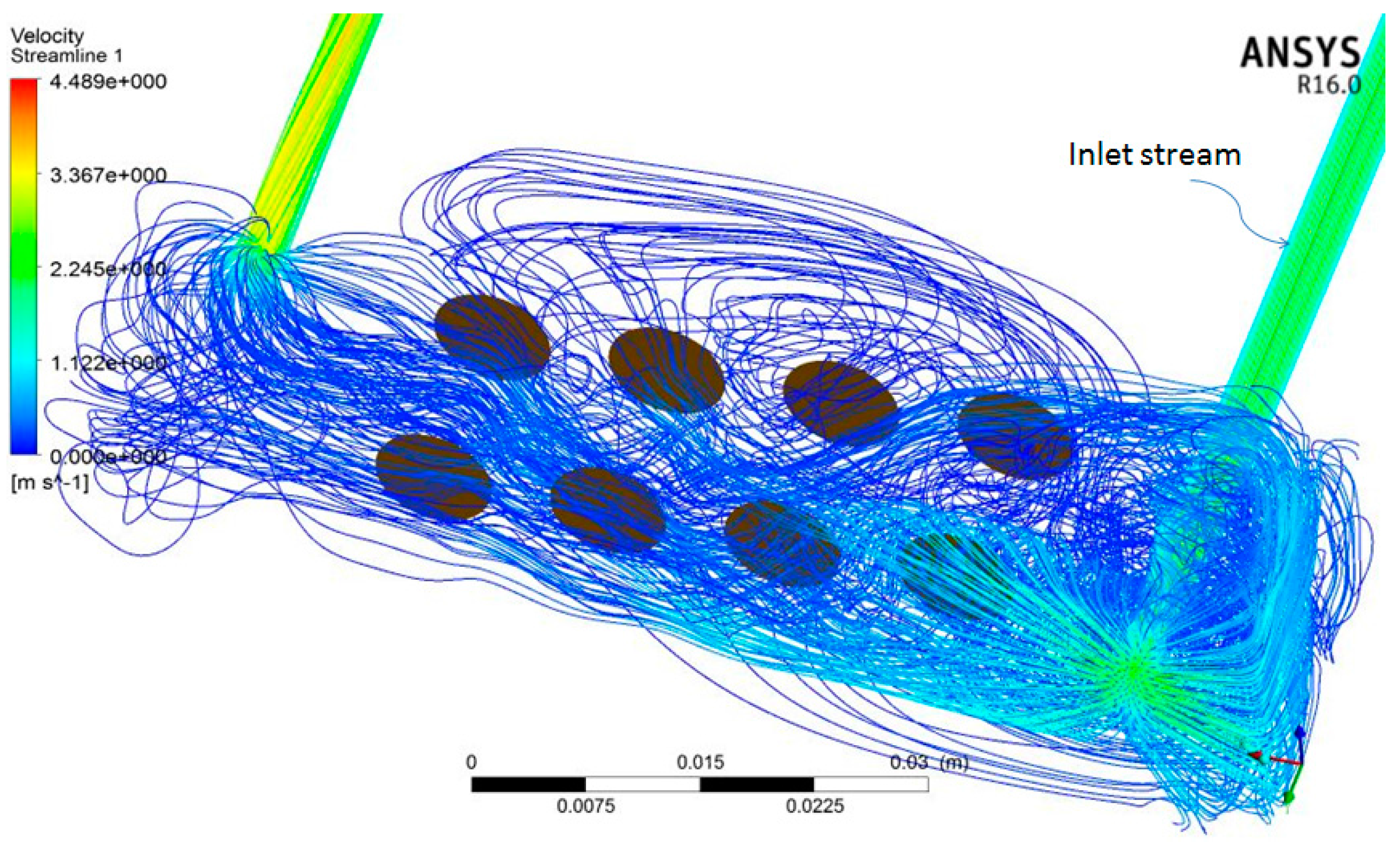
The velocity of the inlet boundary condition was implemented at the inlet of the sensor box and a presumed uniform inlet velocity, 2.4 m/s, corresponding to the real situation at the inlet boundary condition. The type of outlet boundary was set as the pressure-outlet boundary where relative pressure was set to zero in accordance with the real environment. Both the inlet stream and the outlet stream temperature are maintained at 25 °C (room temperature), and the sensor box is fixed at a constant temperature. Furthermore, the gas flow does not slip onto the walls of the sensors and the walls are impermeable. The walls are also held at a constant temperature. Identical wall boundary conditions were also applied at the walls of the sensor box’s cavity.
4.5. Simulation Strategy
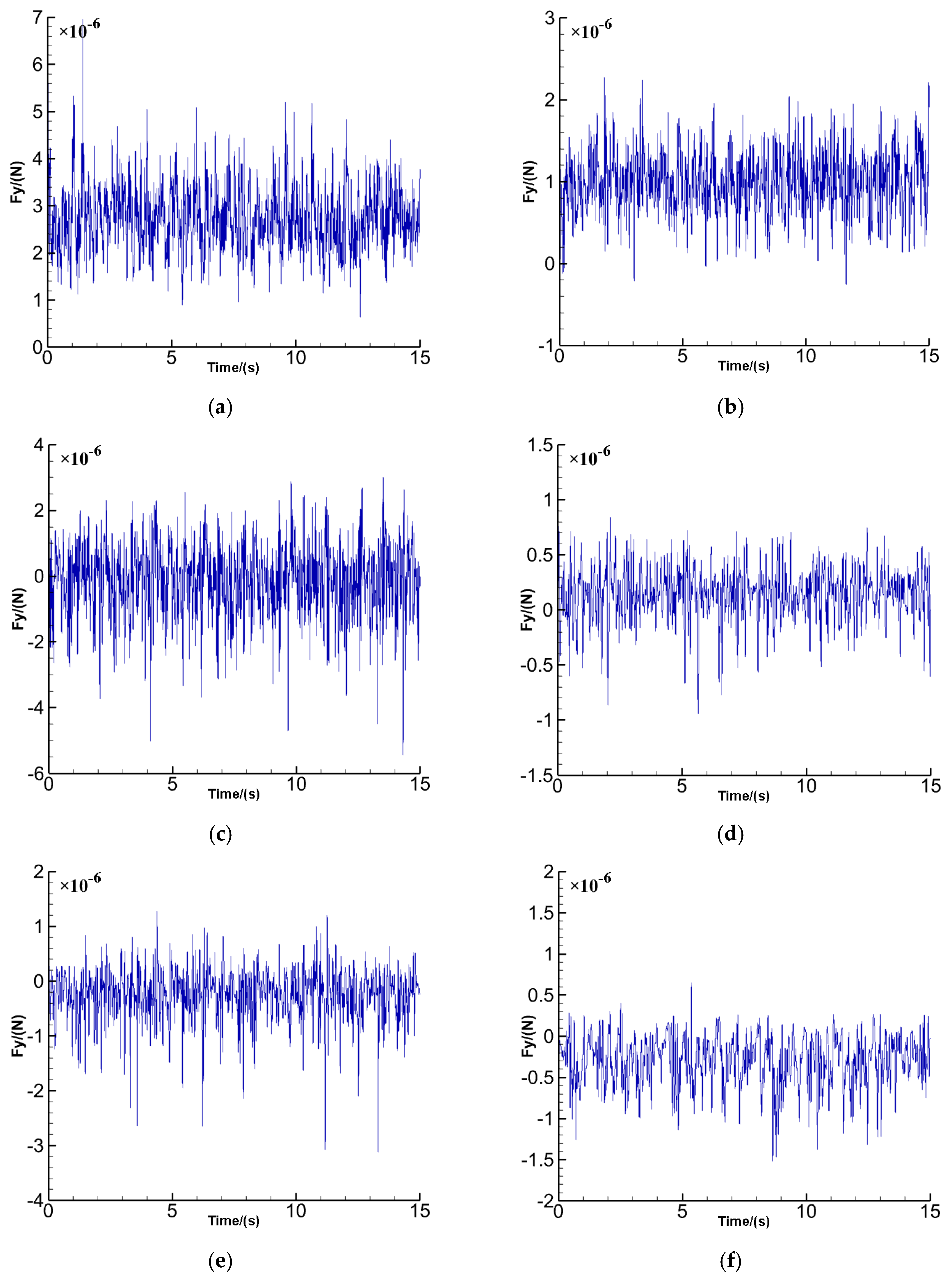
The steady simulation was utilized for studying the grid independence and the unsteady simulation was adopted to model the gas flow in the sensor box, respectively. However, in both the approaches, the steady state solver was initially run for 2000 iterations with de-creased Under Relaxation Factors (URF) from which residuals start exhibiting periodical oscillations. The steady simulation was then solved by further running the steady solver until the monitored facet average static pressure that passed through both the inlet and outlet became stable. The unsteady simulation was run by cutting over to the second order implicit unsteady solver with original default URF and constant time step size of 0.0004 s. The transient runs required 10–20 iterations per time step to reach the desirable residual value 1 × 10⁻⁴. A total number of time steps of 37,500 was used for the full unsteady simulation from 0 s to 15 s.
4.6. The Grid Independence Study
The computational results are greatly influenced by the grid, so the grid independence study should be able to acquire accurate simulation results. The grid independence study was performed by steady simulation. Three levels of mesh containing 2,026,140, 2,529,639 and 3,018,395 cells, for modeling gas flow in the sensor box have been tested, to be sure that the obtained results are grid-independent. The computational results of the three grid types are examined in
Table 5. As seen in the table, the maximum difference between the coarsest and finest grid is less than 1%, so the 2,026,140 cells grid produces grid-independent results. To exclude any uncertainty, computations have been performed using the 2,529,639 cells grid, where the total number of cells was not critical with respect to the computation overhead.
6. Conclusions
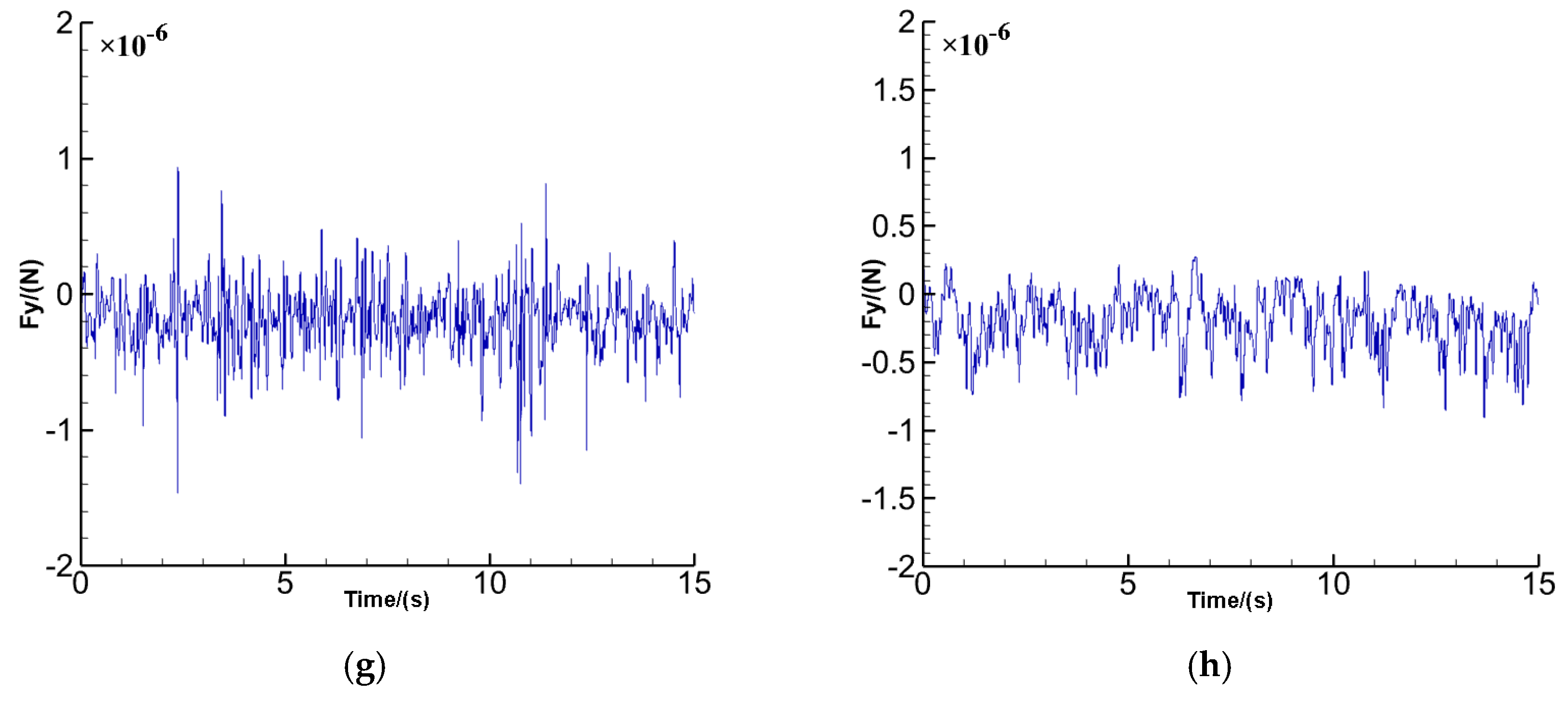
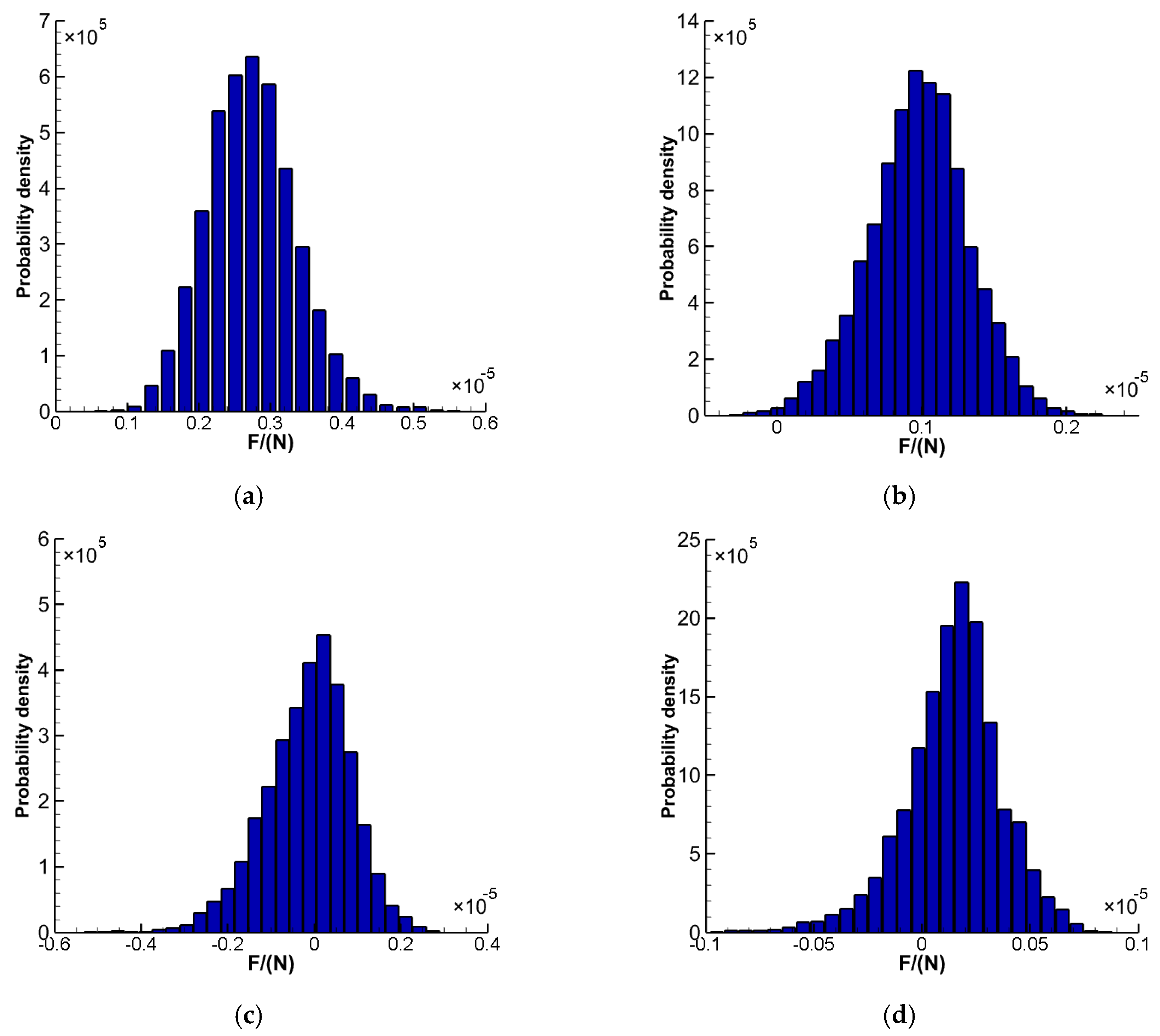
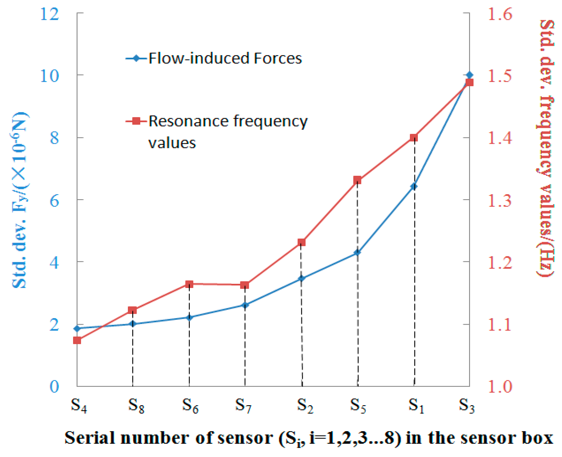
A 3D CFD simulation using the finite volume method is employed to study the flow-induced forces on each sensor in a sensor box. A dedicated procedure was developed for modeling the flow of volatile gas of Maotai (the most famous Chinese liquor) in a realistic scenario to give reasonably good results with fair accuracy. The simulated results illustrated that a strong swirling flow is formed near the intake tube, which is explained by the inlet stream's impact on the wall. The resultant force () values on each sensor in the y-direction were recorded at every time step during the numerical simulation. Under the influence of the gas flow, the probability density distributions of the Fy on each sensor are close to the standardized Gaussian distribution. We obtained the standard deviation () of the Fy from “sensor 1” to “sensor 8”. Comparing the standard deviation between the Fy and the resonance frequency values of each sensor, the results show that the fluctuations of Fy are bound up with the resonance frequency values fluctuations. When the fluctuations of Fy are stronger, the fluctuations of the resonance frequency values are more obvious. However, when the fluctuations of Fy are not strong, the fluctuations of resonance frequency values are affected slightly. The conclusion shows that, for the resonance frequency values fluctuation of the sensors at stable state, the influence of the flow-induced forces should not be neglected. To ensure that the sensor's resonance frequency values are steady and do not fluctuate significantly, in order to improve the identification accuracy of Chinese liquors using the e-nose, the sensors in the sensor box should be in the proper place, i.e., where the fluctuations of the flow-induced forces is relatively small. The results play a significant reference role in determining the optimum design of an e-nose for accurately identifying Chinese liquors.


