1. Introduction
Polarimetric synthetic aperture radar (PolSAR) is popular and attractive due to its advantage of providing richer information with four channels HH, HV, VH and VV, where HH, HV, VH and VV denote the polarization models for horizontal transmit and horizontal receive (HH), horizontal transmit and vertical receive (HV), vertical transmit and horizontal receive (VH), and vertical transmit and vertical receive (VV), respectively. Many researches have been developed on PolSAR images. Among them, PolSAR image classification [
1,
2,
3,
4,
5] is a basic issue. There are basically two approaches for classification: (1) pixel-based classification; (2) region-based classification. Due to the presence of inherent speckle noise in PolSAR images, traditional pixel-based classification algorithms have some drawbacks [
6], i.e., sensitivity to noise and more computation. Compared to the traditional pixel-based methods, region-based algorithms process images at region level instead of pixel level, making the information of regions more available with better anti-noise performance. However, additional region generation methods are generally required beforehand, e.g., superpixel algorithms.
Ren and Malik [
7] firstly proposed the term superpixel—a group of pixels with similar color or other low-level features—in 2003. Superpixels have been commonly used for a wide range of applications, for example, as a preprocessing step for change detection [
8,
9], as mid-level cues used for tracking [
10], or as a preprocessing step for classification [
11,
12,
13]. So far, many superpixel segmentation algorithms have been proposed, which can be generally categorized into two classes: graph based methods and gradient ascent methods. Normalized Cuts (Ncut) [
7], Entropy Rate Superpixels [
14] and Pseudo Boolean Optimization (PB) [
15] are the typical algorithms of graph based methods. For gradient ascent methods, there are QuickShift (QS) [
16], Contour Relaxed Superpixels (CRS) [
17] and Superpixels Extracted via Energy-Driven Sampling (SEEDS) [
18]. Simple Linear Iterative Clustering (SLIC) [
19], which is popular for its simplicity and good performance, can also be classified into the gradient ascent methods. All the algorithms mentioned above are originally proposed for optical images and have their own advantages for different images. However, when applied to PolSAR images, they may generate poor superpixels because of the serious influence of inherent speckle noise and many small-sized or slim regions in PolSAR images.
SLIC is attractive and contains three main steps: (1) initialization; (2) local k-means clustering; (3) postprocessing. Zou et al. [
20] proposed an improved SLIC based on generalized Gamma distribution for SAR images. While the algorithm shows good performance in SAR data, it does not do so PolSAR data. Recently, many improved algorithms based on SLIC have been proposed for PolSAR images. Feng et al. [
21] introduced an improvement over SLIC by utilizing the Wishart distance instead of color Euclidean distance. Although the algorithm yields better superpixels than SLIC, small isolated regions still exist and the computation efficiency is unsatisfactory. Another method based on SLIC, which employs a combined distance, including space distance, Wishart distance and edge gradient distance, was proposed by Xie et al. [
9]. This method can preserve the edges very well, but with low computation efficiency. Qin et al. [
22] proposed an improved SLIC based on the revised Wishart distance and improved postprocessing. The final superpixels are of good boundary adherence but with long running time and unsatisfactory regularity. Zhu et al. [
23] introduced a fast superpixel segmentation algorithm by iterative edge refinement (IER), which is fast, homogeneous regular and boundary-adherent for optical images. However, IER cannot be directly applied to PolSAR images to yield superpixels due to the strong impacts of coherent speckle noise interference in PolSAR images.
To address these problems—inspired by the work in the literature [
23]—an improved SLIC algorithm is proposed to generate fine superpixels for PolSAR images in this paper. Different from the IER originally designed for the superpixel generation of optical images, in the initialization step of our improved algorithm, we initialize unstable pixels as all the pixels in PolSAR images rather than the initial grid edge pixels in IER, so as to maintain all the potential edge pixels to eliminate the effects of small-sized or slim regions in PolSAR images. Moreover, when relabeling the unstable pixels in the local searching area, the revised Wishart distance, instead of Euclidean distance, is adopted as the data distance measure to reduce the impact of speckle noise. In the literature [
24], a fast PolSAR image classification was proposed based on fast implementation of Wishart distance. Inspired by this, the revised Wishart distance is calculated by fast implementation to further increase computation efficiency. Finally, postprocessing with a dissimilarity measure is utilized to remove the generated small isolated regions and to preserve strong point targets at the same time. Four simulated and two real-world PolSAR images are exploited to evaluate the superior performance of the proposed method. The experimental results indicate that the proposed method may obtain better performance with respect to several commonly used evaluation measures with higher computational efficiency, as well as more accurate boundary adherence and strong point targets preservation, compared with three state-of-the-art methods.
2. IER for Optical Images
IER is a fast superpixel generation algorithm and shows fine performance when applied to optical images. In an image, unstable pixels [
23] are those pixels whose labels are likely to change and should be checked in the next iteration. The definition of unstable pixels is given as follows:
where
and
represent pixels in the image domain
, i.e.,
.
is the neighborhood function and a 4-connected neighborhood is utilized in the experiments.
represents the label of
and
represents the new label after one iteration,
.
The color-spatial combined distance [
25] is used in IER to relabel the unstable pixels in the local clustering and LAB color space developed by International Commission of Illumination (CIELAB) is employed. The combined distance is defined by
where the subscripts
and
represent the cluster center of the
superpixel and the
unstable pixel, respectively.
is the initial grid width and
is the compactness parameter. When
is a large value, it indicates that the spatial distance is more significant than the data distance, thus leading to more regular final superpixels. The main steps of the IER algorithm are shown in Algorithm 1:
| Algorithm 1. IER for Optical Images. |
| given: the initial grid width , color image |
| step 1. (Initialization) |
| Initialize the superpixels of as regular grids with width . Create the models (mean color values and geometric centers) for all superpixels. Initialize the unstable pixels as the grid edge pixels. Set the iteration index iter = 0. |
| step 2. (Local relabeling) |
| If iter ≥ itermax, the maximum iteration times reached, or the unstable pixel set is empty, then the algorithm ends and goes to Step 4. If not, relabel all the unstable pixels by the color-spatial combined distance defined in Equation (2) in the local searching area . |
| step 3. (Updating) |
| Update the superpixel models and the unstable pixel set by its definition (1). Set iter = iter + 1 and return to Step 2. |
| step 4. (Postprocessing) |
| Remove the generated isolated regions with size smaller than by connected component analysis (CCA) based on the combined distance defined as Equation (2). |
| output: superpixels |
3. Proposed Superpixel Algorithm
IER is originally proposed to generate superpixels efficiently for optical images. However, when applied to PolSAR images, IER may generate poor superpixels due to the influence of inherent speckle noise and many small-sized or slim regions. In
Section 3.1 we introduce the revised Wishart distance to replace the CIELAB Euclidean distance as the data distance measure. By doing so, the effect of speckle noise will be reduced significantly.
Section 3.2 contains the initialization step of the proposed method for PolSAR images with many small-sized or slim regions. In
Section 3.3, a postprocessing procedure based on the dissimilarity measure is introduced to remove the generated small regions as well as to preserve the strong point targets. Finally, the algorithm flow is given in four steps. Since our proposed method is motivated by the IER algorithm originally designed for the superpixel generation of optical images and is applied to PolSAR images in this paper, we call it Pol-IER for simplicity hereafter.
3.1. Revised Wishart Distance
3.1.1. Traditional Revised Wishart Distance
The amplitude and phase of backscattering signals, which are in four combinations of linear, receive and transmit polarizations: HH, HV, VV, VH; usually contained in PolSAR data. Each pixel of a PolSAR image can be described by a complex matrix as follows:
where
for a reciprocal medium. Generally, Pauli scattering vector
can be used to represent the backscattering signals. It is defined by
where the superscript
denotes the matrix transpose. For multilook PolSAR data, the polarimetric information can be described as the coherency matrix
, which can be generated from the outer product of
. The expression can be denoted by
where
is the number of looks and the superscript * denotes the complex conjugate. Let
. Then
has the complex Wishart distribution [
26], i.e.,
, where
. Therefore, the probability density function (PDF) of
is given by
where
is the Gamma function [
27] and
is the dimension of
, i.e., 3.
is the determinant of a matrix. Thus the PDF of
can be written as follows:
Let
and
be the center coherency matrices of the regions
and
, respectively. The hypothesis test [
28] is
Then the maximum-likelihood (ML) estimators of
and
are
and
, respectively. When
is given for hypotheses
and
, the likelihood-ratio test statistic [
22] is
Thus, the distance between
and
is the revised Wishart distance [
26] defined by
So the revised Wishart distance between a pixel
with the coherency matrix
and the
cluster
with the center coherency matrix
is
In this paper, Equation (14) is utilized instead of
in Equation (4) to eliminate the influence of speckle noise in the step of local relabeling. In some literatures [
21,
29,
30], Wishart distance defined as Equation (15) is employed to measure the distance between a pixel and a cluster. Our experiments on the simulated PolSAR data will illustrate that our algorithm with the revised Wishart distance outperforms the Wishart distance in terms of four commonly used criteria.
Therefore, the combined distance of the pixel
i and the cluster
used in this paper is
3.1.2. Fast Implementation of Revised Wishart Distance
Since the revised Wishart distance will be calculated many times in the local relabeling step, a large amount of time will be spent in the computation of the distance. Therefore, a fast implementation [
24] of the revised Wishart distance is employed in this paper to further increase the computation efficiency. As shown in Equations (14) and (15), the term
is traditionally calculated by multiplying
by the matrix
firstly and then computing the trace of the matrix
, which needs 27 multiplication operations and 20 addition operations with the obtained
. Let
. It is known that both
and
are
complex matrices, and so is
. To calculate the trace of
, we only need to summarize the diagonal elements of
. That is to say, it is redundant to calculate the matrix
and only necessary to obtain the diagonal elements. Therefore, the fast implementation of the revised Wishart distance is only to calculate the summary of the diagonal elements and leave out the redundant computation.
Based on the idea mentioned above, let
be a function that arranges all the elements of the matrix
into a vector. In this paper,
and it is noticed that
and
are conjugate symmetry for the coherency matrix
. Let
and
, where
means a matrix transpose without conjugation. Then it is easy to notice the fact that
, where both
and
are 9-dimensional vectors. Contrary to the high-computation of
, only nine multiplication operations and eight addition operations are needed to calculate
, which is only one-third of what
the traditional way needs. Therefore, the revised Wishart distance can be represented by
3.2. Initialization of Unstable Pixels
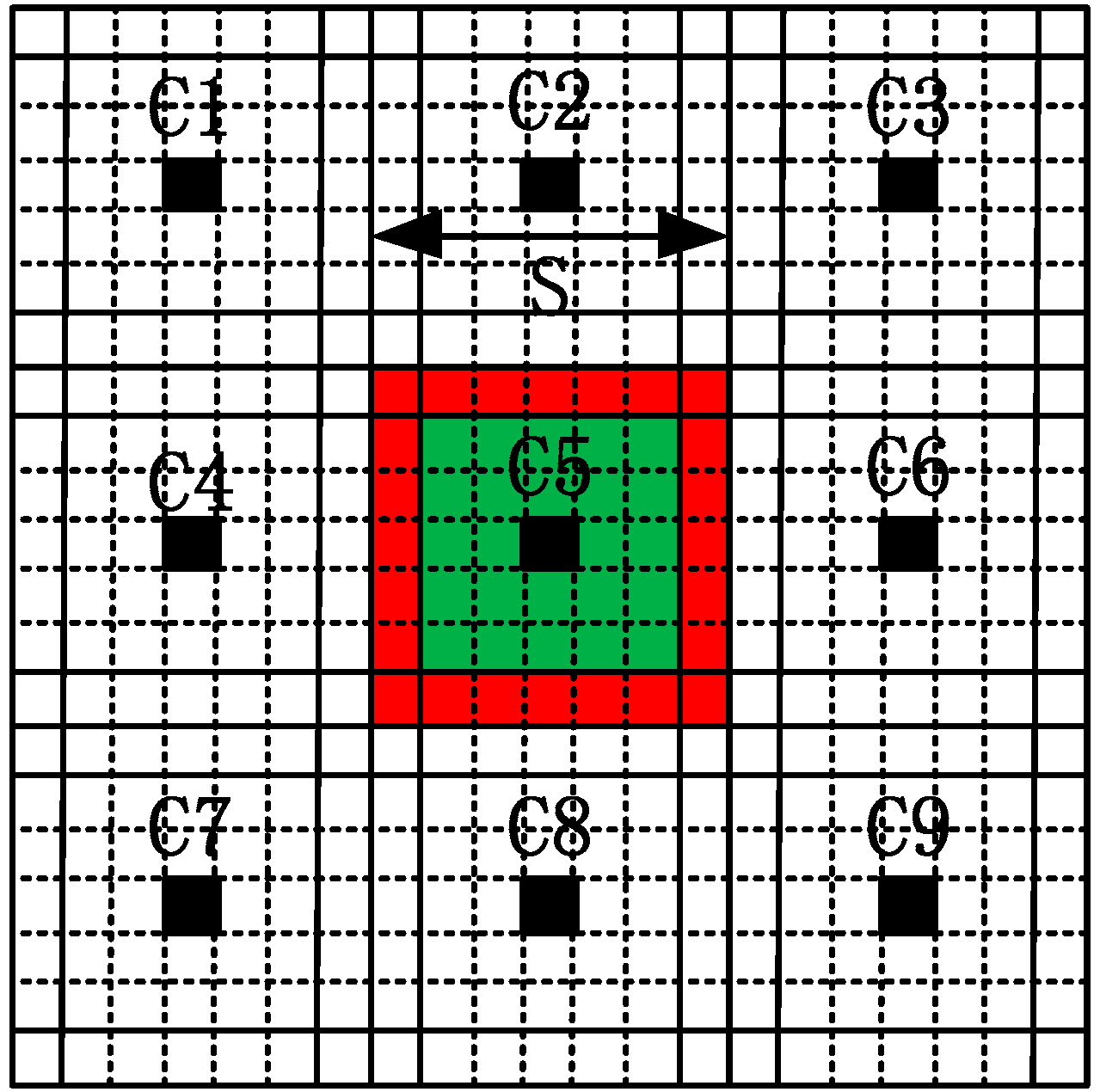
As shown in
Figure 1, to generate superpixels using IER, an image is firstly divided into several grids with width
. For example, for the fifth cluster, the original center is set as
, i.e., the pixel filled with black. The IER algorithm initializes the unstable pixels as the regular grid edge pixels, for example, the red pixels in the edge of the fifth cluster. For optical images, this kind of initialization has a slight effect on the boundary adherence of the final superpixels, because optical images always contain several regions of regularity and homogeneity. By contrast, PolSAR images usually include many small regions, slim regions and strong point targets, which provide important information for image processing such as ship detection, change detection and classification of land use/land cover (LULC), and so on.
When applied to PolSAR images, IER with this kind of initialization may yield poor superpixels with many edges lost. In addition, the properties of good boundary adherence and homogeneous regularity should be obtained with as few superpixels as possible. This means that whether the final superpixels are good or not does not depend on the initial grid width. However, the final results of IER can be severely affected by the initial grid width. Since many real edge pixels may locate in the middle of the grid, when the original grid width is large relative to the image size, some true edges may be missed with this kind of initialization. Therefore, with a small grid width, IER may work well, and otherwise the opposite, which is not expected.
To fix the problems mainly caused by the initialization of IER for generating superpixels for PolSAR images, we initialize the unstable pixels as all the pixels in PolSAR images instead of the initial grid edge pixels. For the fifth cluster in
Figure 1, our proposed initial unstable pixels consist of the red pixels, green pixels and the corresponding cluster center filled with black. By doing so, all the potential edges in PolSAR images will be maintained, resulting in accurate boundary adherence and thus accurate superpixels. Although the initialization step of our proposed method will slightly increase the running time at the first several iterations (Usually three or four iterations. See
Section 4.1.2 for more details), we can ensure the preservation of all the potential edges, which is of significance for superpixels’ applications.
3.3. IER for PolSAR Data
Based on the above analysis, the IER for PolSAR data in this paper can be summarized as three steps to generate superpixels. Although some changes have been made based on the characteristics of PolSAR images, small isolated superpixels may still exist. To address this problem, the connected components algorithm (CCA), based on the combined distance in Equation (4) to remove small isolated regions by merging them into nearby large superpixels, is used in IER. Although it is easy to perform, it will lead to poor boundary adherence of superpixels for PolSAR images. That is because the generated small isolated regions may significantly differ from the adjacent superpixels.
In order to merge the generated small isolated regions as well as to preserve the strong point targets, a postpocessing procedure [
21] based on a dissimilarity measure is introduced in this paper. The superpixels with the size smaller than the prespecified threshold
are interesting. When the size of a superpixel is smaller than
, the dissimilarities between this superpixel and the superpixels in its 8-connected neighborhood will be calculated. If the smallest dissimilarity value is smaller than a predefined threshold
, we merge this superpixel into the neighbor with the smallest dissimilarity between them. If not, move to the next superpixel. The dissimilarity measure [
14] between two superpixels
and
is defined as follows:
where
means the vector consisting of the diagonal elements of the center coherency matrix of a superpixel and
denotes 1-norm of a matrix. Since the dissimilarity
belongs to [0, 1],
is set as 0.3 in all the experiments throughout this paper.
The main steps of our improved IER for PolSAR data, namely Pol-IER, can be summarized in Algorithm 2.
| Algorithm 2. Pol-IER for PolSAR images. |
| given: the initial grid width , PolSAR image |
| step 1. (Initialization) |
| Initialize the superpixels of image as regular grids with interval . Create the models (mean coherency matrices and geometric centers) for all the superpixels. Initialize the unstable pixels as all the pixels of the PolSAR image. Set the iteration index iter = 0. |
| step 2. (Local relabeling) |
| If iter ≥ itermax, the maximum iteration times reached, or the unstable point set is empty, then the algorithm ends and goes to Step 4. Or relabel all the unstable pixels by the combined distance defined in Equation (16). Assign each unstable pixel whose searching area is to the closest cluster whose location is covered by the searching area. |
| step 3. (Updating) |
| Update the superpixel models and the unstable pixel set by the definition (1). Set iter = iter + 1 and return to Step2. |
| step 4. (Postprocessing) |
| Search the superpixels with the size smaller than . If the smallest dissimilarity calculated by Equation (18) is smaller than , merge it into the closest adjacent superpixel. If not, move to the next superpixel until each superpixel is checked. |
| output: superpixels |
4. Experiments and Discussion
To evaluate our proposed Pol-IER, extensive experiments on four simulated PolSAR images and two real-world images from Experimental Synthetic Aperture Radar (ESAR) and Airborne Synthetic Aperture Radar (AirSAR) were conducted.
Section 4.1 introduces four commonly used criteria: comparison experiments of the Wishart distance, and the revised Wishart distance; evaluations on two initialization methods; and comparison experiments on four state-of-the-art algorithms (i.e., the standard SLIC, IER, SLIC-GC [
22] and Pol-IER) based on the simulated PolSAR data. The experiments demonstrate that the proposed method shows good performance with respect to the four criteria. In
Section 4.2, experiments and discussions on two real-world PolSAR images are contained and the results show that the proposed method works best on boundary adherence and strong point targets preservation with higher computation efficiency compared with three state-of-the-art methods, i.e., the standard SLIC, IER and SLIC-GC. All the experiments were performed on a personal computer with 3.30 GHz Intel Pentium CPU, 4 GB memory and Matlab Code.
4.1. Evaluation on Simulated PolSAR Images
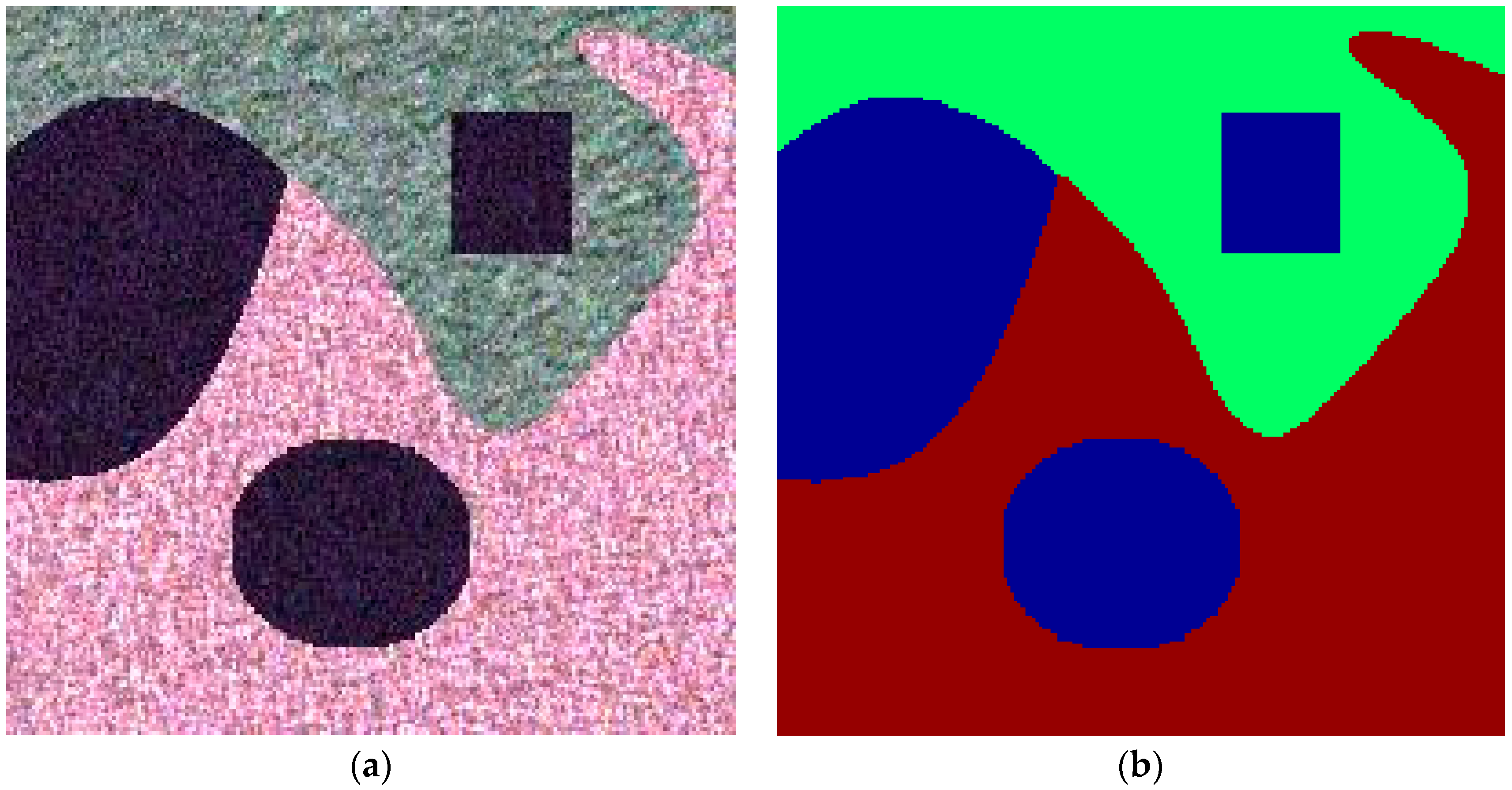
In our experiments, to evaluate the algorithms quantitatively, four simulated PolSAR images with three same regular regions but different sizes, i.e.,
,
,
, and
pixels, were employed. The generation of simulated PolSAR images is based on the inverse transform method [
31]. The simulated image with size
pixels is shown in
Figure 2a and the corresponding ground truth is given in
Figure 2b.
To evaluate the performance of different methods for superpixels’ generation, all the experiments on the four simulated PolSAR images mentioned above were assessed on four commonly used criteria: Boundary Recall (BR), Under-segmentation Error (USE), Achievable Segmentation Accuracy (ASA) and the running time. BR, USE and ASA are defined as follows:
Boundary Recall [
32]: BR is the ratio of boundary pixels shared by the obtained superpixels and the ground truth, and it can be represented as
where
denotes the number of superpixels’ boundary pixels overlapping the ground truth edges, and
represents the number of ground truth edges. In this paper, the internal boundaries of the ground truth and superpixels were employed. So for BR, a larger value means better results.
Under-segmentation Error: if the ground truth segments are
and the obtained superpixels are
, the under-segmentation error is defined by [
19,
25]:
where
is the number of all the pixels in an image,
is the overlapping error of the superpixel
relative to a ground truth segment
.
denotes the size of superpixels, and
represents a minimum number of pixels in
overlapping
. So USE should be as low as possible to obtain good superpixels.
Achievable Segmentation Accuracy [
14]: ASA is a performance upperbound measure and the highest achievable accuracy of object segmentation when utilizing superpixels as units. By labeling each superpixel with the label of the ground truth segment that has the largest overlap, ASA can be computed as the fraction of correctly labeled pixels.
4.1.1. Evaluation on Two Distance Measures
In this paper, the fast revised Wishart distance instead of Wishart distance is employed as the data distance measure. Comparison experiments of our method with two distances were conducted on the four simulated PolSAR images to illustrate the superiority of the fast revised Wishart distance in our method.
The compactness parameter
was set as 1.4 (the best) for the revised Wishart distance and 1 (the best) for the Wishart distance. The results on the four criteria are shown in
Figure 3. We can find that the fast revised Wishart distance in our method was greatly superior to the Wishart distance in terms of all the four criteria. This is because the revised Wishart distance can better characterize the real data distance between coherency matrices than the Wishart distance and the fast implementation of the revised Wishart distance can significantly increase the computation efficiency. In addition, BR, USE, ASA and running time change very slightly with different initial grid width
, which is the expected property for superpixels. Therefore, the fast revised Wishart distance is chosen as the data distance measure in our proposed Pol-IER method.
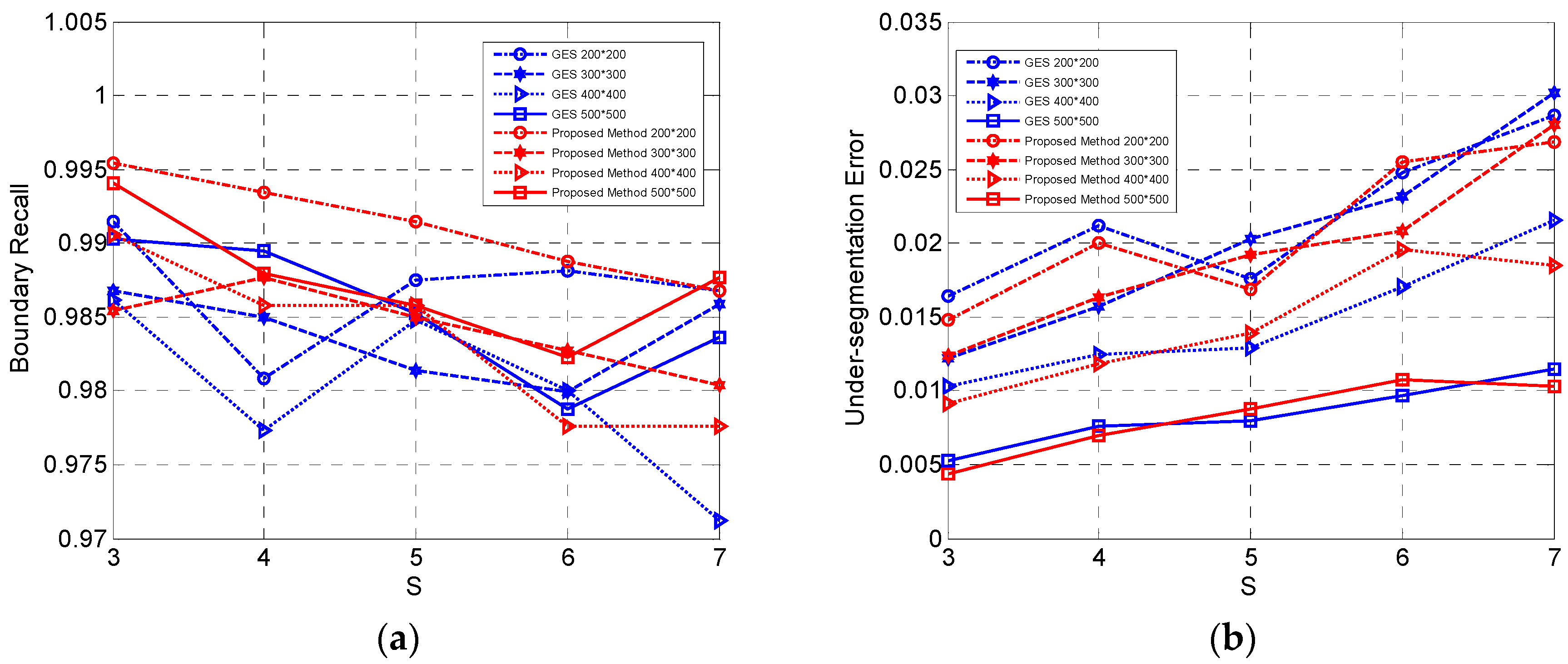
4.1.2. Evaluation of the Proposed Initialization Method
The initialization of unstable pixels is set as all the pixels instead of the grid edges scheme (GES) in IER. To demonstrate the advantage of the proposed initialization method, these two methods of initializing unstable pixels with the same steps were compared.
The comparison results are shown in
Figure 4.
Figure 4a–c shows the slight advantage of our method in terms of BR, USE and ASA. That is because our method of initialization is proposed for those images with small-sized or slim regions which are common in real-world PolSAR images. The regions of simulated images are large and regular, thus leading to a small advantage for our initialization method. The superiority will be further shown in the experiments on the real-world PolSAR images in
Section 4.2. The running time of our initialization with a larger number of initial unstable pixels is longer than the GES as shown in
Figure 4d. The curves of unstable-pixels-to-all-the-pixels ratio with the iterations increasing are given in
Figure 4e,f.
Figure 4e,f is the results of the simulated PolSAR images with sizes
and
pixels, which are the smallest and largest size in all the represented simulated images, respectively. It can be seen that the ratio of the proposed method decreases more quickly than that of the GES and that the two methods will maintain a similar number of unstable pixels after three or four iterations. Therefore, the computation time is mainly spent on the first few iterations in Pol-IER, because the unstable pixels, of which most are the edges according to definition (1), are almost fixed in an image. Although our method takes a little longer, the curves change more slowly with different initial grid width compared with the GES, which means that the generated superpixels can maintain similar properties with different a grid width
. In addition, it can be seen from
Figure 4d that the running time gap between our algorithm with the two initialization method will be widened with the size of PolSAR images increasing. This is mainly because when the size of the image is small, the initial unstable pixels to be relabeled in our method are of a small number, but with the large size of images to process, more pixels need to be relabeled by Pol-IER in the first few iterations. In summary, our proposed method of initialization outperforms the GES in terms of the expected properties with a little longer running time.
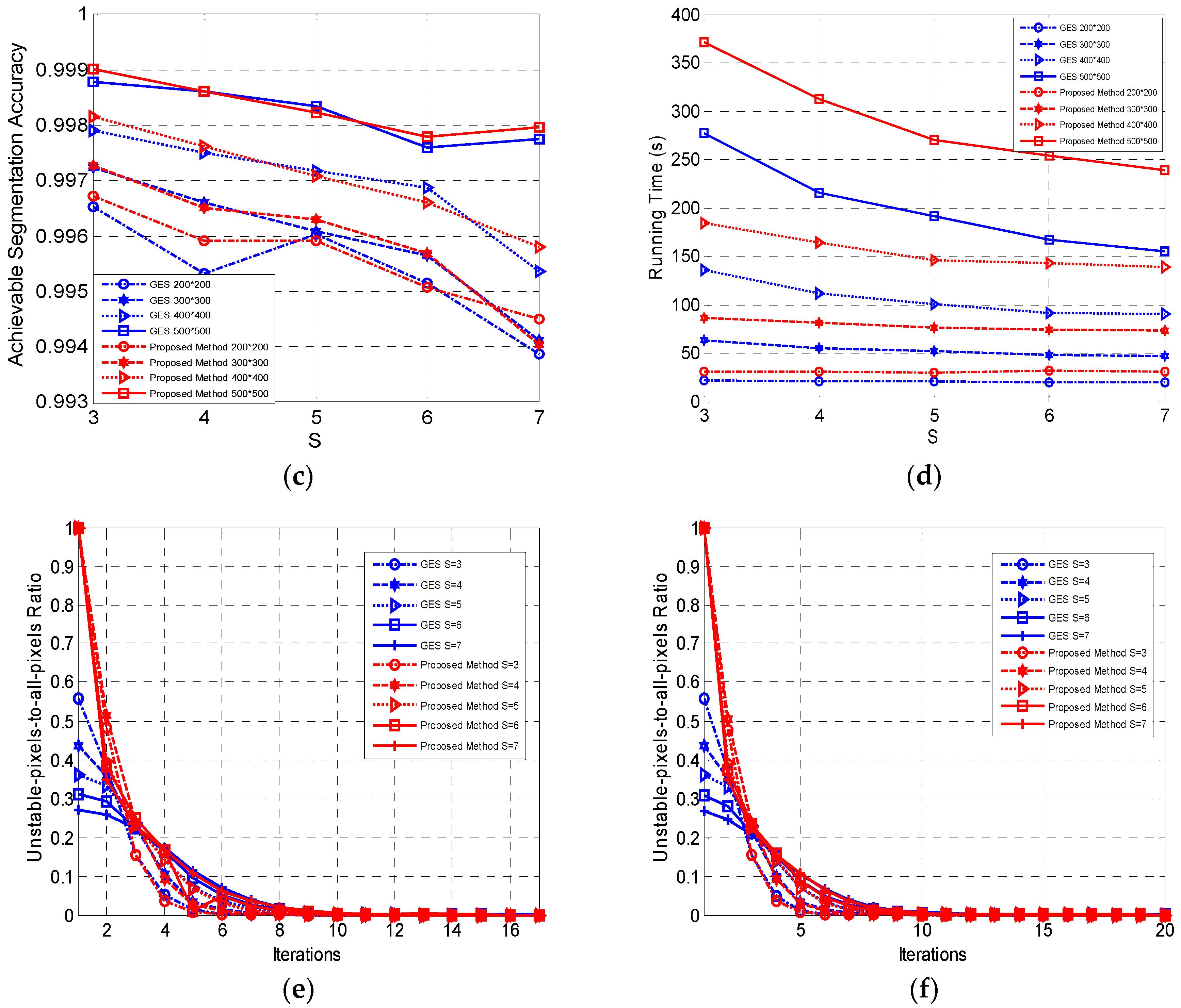
4.1.3. Evaluation on Four Algorithms
Four algorithms including the standard SLIC, IER, SLIC-GC and Pol-IER were evaluated on the four simulated images. For these methods, a sequence of initial grid widths was set as for wider comparison. The compactness parameter was set as 15 for the standard SLIC and IER, 1.2 for SLIC-GC, and 1.4 for Pol-IER. Both and were set as in the experiments.
Figure 5 illustrates the results of the four algorithms on the four simulated images. The BRs of three methods, i.e., IER, SLIC-GC and Pol-IER are shown in
Figure 5a, which does not include the BR of the standard SLIC for clarity because of the small value, about 10% lower than the other three algorithms. For BR, SLIC-GC outperforms IER, and Pol-IER is the best of the results, which indicates that the superpixels generated by Pol-IER have the boundaries closest to the real edges among the four methods.
Figure 5b is the USEs of three algorithms similar to
Figure 5a. The USE of the standard SLIC, which is the worst and thus not included in
Figure 5b for clarity, is about 1.5% larger than those of the other three methods. IER is the second worst with a larger USE than SLIC-GC. As shown in
Figure 5c, ASA has the same performance as the USE. Both the standard SLIC and IER utilize CIELAB Euclidean distance, which is unsuitable to describe the PolSAR data, thus leading to the worst BR, USE and ASA for them. Since the revised Wishart distance is employed in SLIC-GC and Pol-IER, SLIC-GC and Pol-IER obtain similar performance in terms of the three criteria, i.e., BR, USE and ASA. Although the USE and ASA of Pol-IER are generally slightly worse than that of SLIC-GC, Pol-IER, with the larger image size and small step, is comparable to SLIC-GC, whose running time is about one order of magnitude higher than that of Pol-IER with a large-sized image as shown in
Figure 5d, where the running time curves of SLIC-GC on images with sizes
,
and
pixels are not included for clarity due to the values that are more than 10 times larger than other results . This is because the properties of superpixels generated by Pol-IER change slowly with different grid widths due to the initialization. With the same running time, Pol-IER can generate superpixels with a small
, which will lead to good performance, but IER can only employ a much larger
, with which poor superpixels will be yielded. Therefore, Pol-IER outperforms the others on overall performance.
4.2. Evaluation on Real-World PolSAR Images
To further evaluate the performance of Pol-IER, two real-world PolSAR images from ESAR and AirSAR were ultilized to conduct experiments. The first PolSAR data set is an L-band PolSAR image from the Oberpfaffenhofen test site, Oberpfaffenhofen, Germany. A preprocessing of six looks in the azimuth and three looks in the range were performed to equalize the resolutions of the azimuth and the range. After the multilook processing, the size is 469 × 513 pixels, and the Sinclair color-coded image is shown in
Figure 6. The second data set is a 4-look AirSAR L-Band PolSAR image with size
pixels from Flevoland, the Netherlands, and the Sinclair color-coded image is shown in Figure 11a.
The standard SLIC, IER, SLIC-GC and Pol-IER were performed on these two real-world images for comparison. The initial grid width is generally set according to the complexity of terrains empirically. In the experiments, all of the initial grid widths were set as for the first data set and for the second one. was set as in CCA and was also set as for SLIC-GC and Pol-IER. The performance of these four competitive algorithms on real-world PolSAR images were visually inspected due to the absence of the ground truth of the real-world images. Therefore, we focused on the performance of the boundary adherence and strong point targets preservation for comparison.
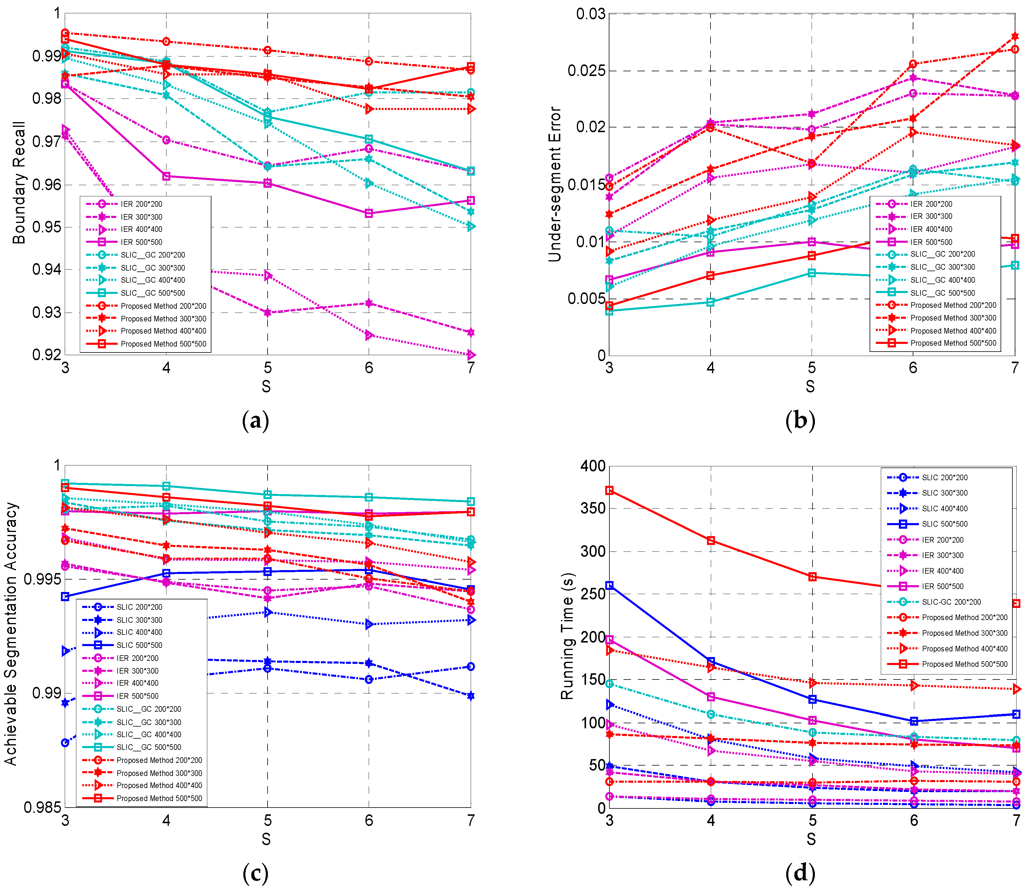
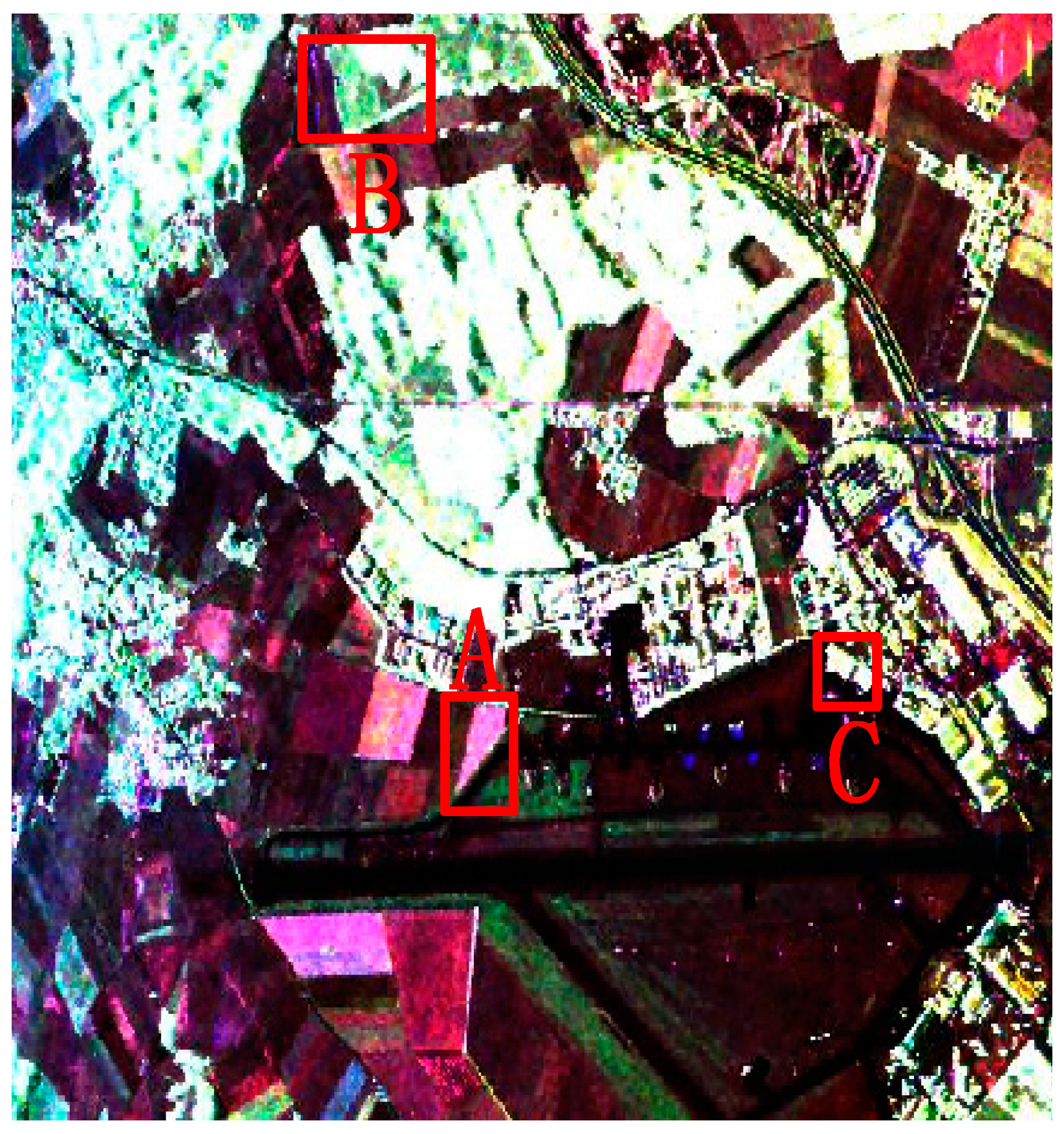
4.2.1. Evaluation on the First Data Set
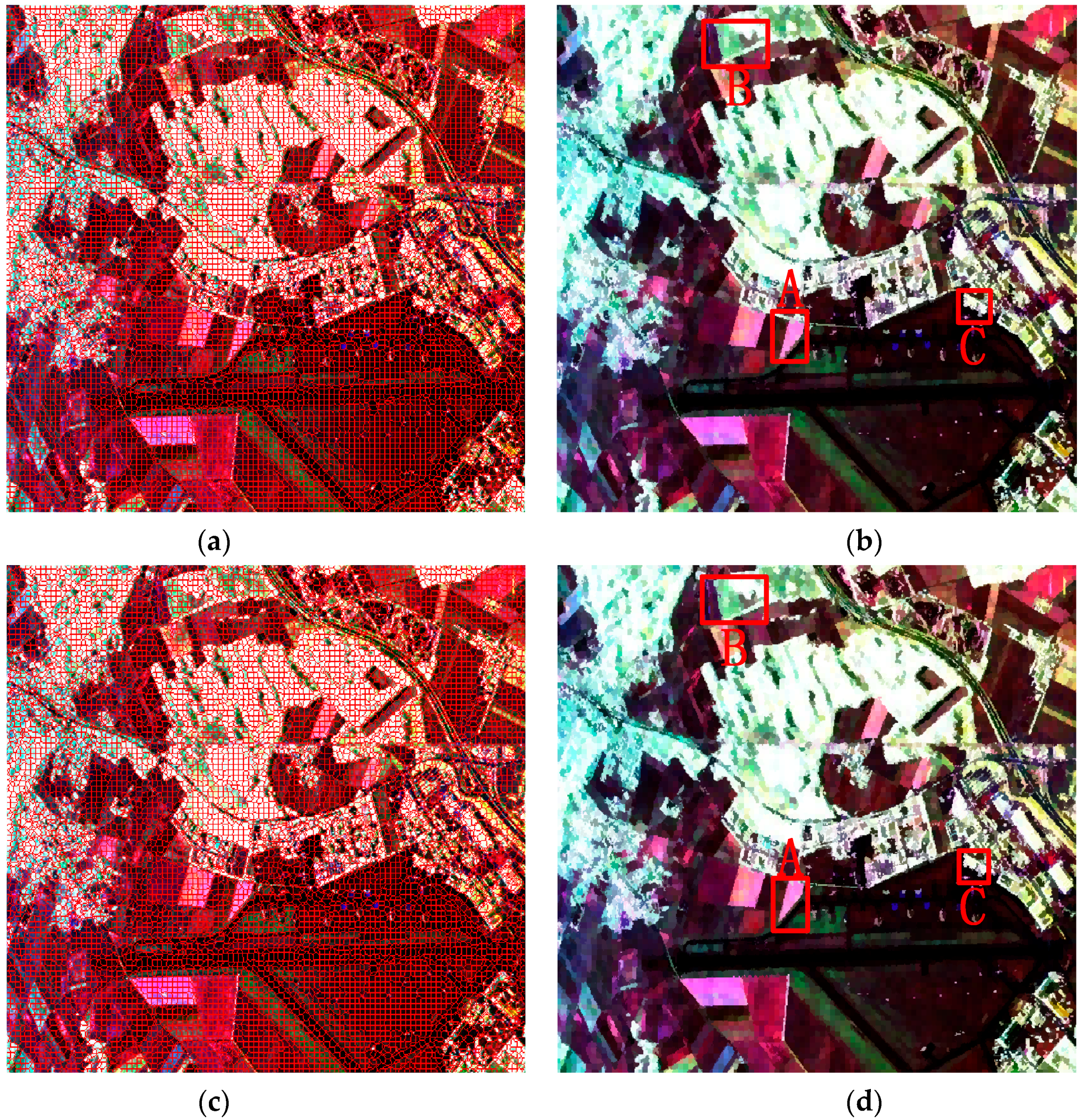
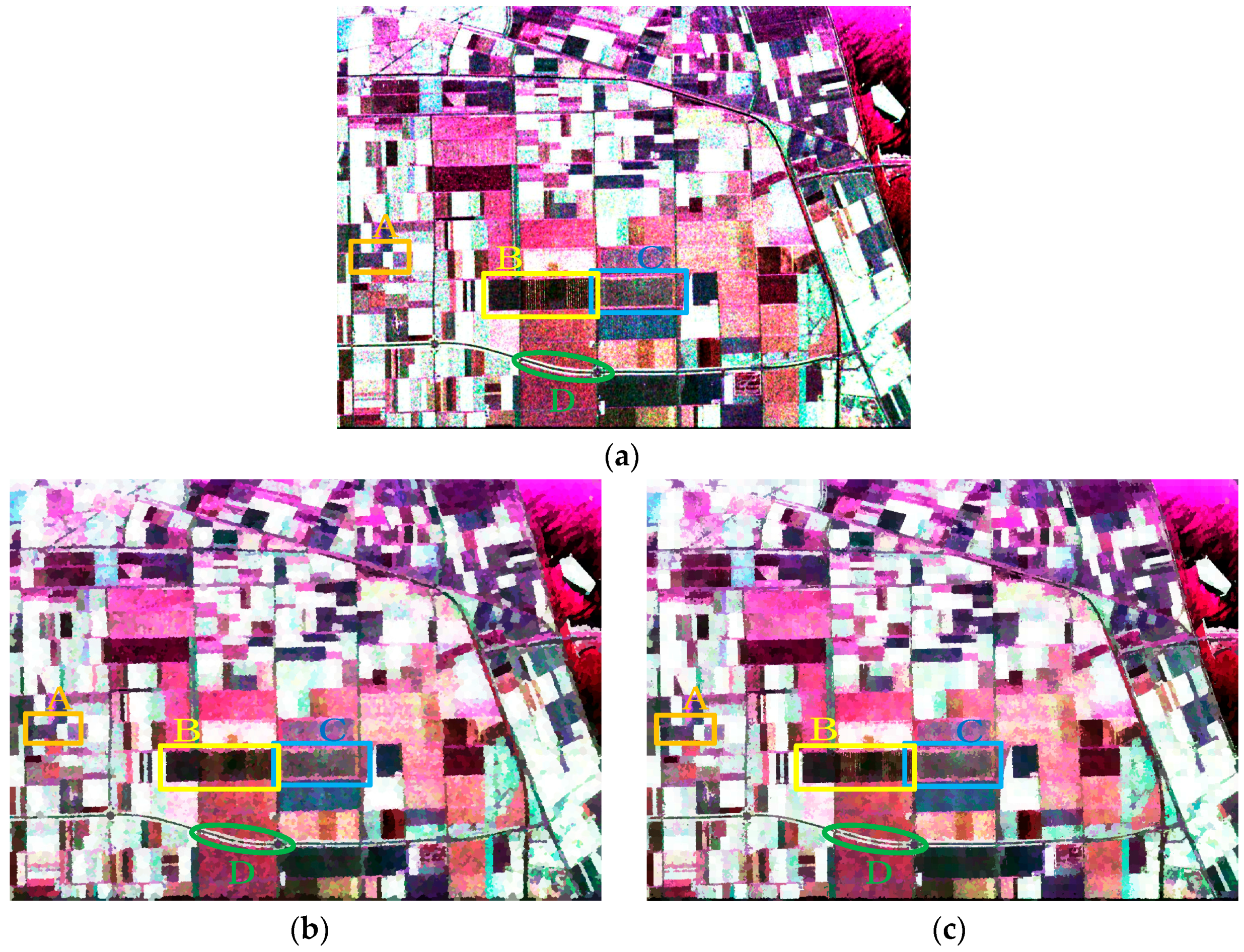
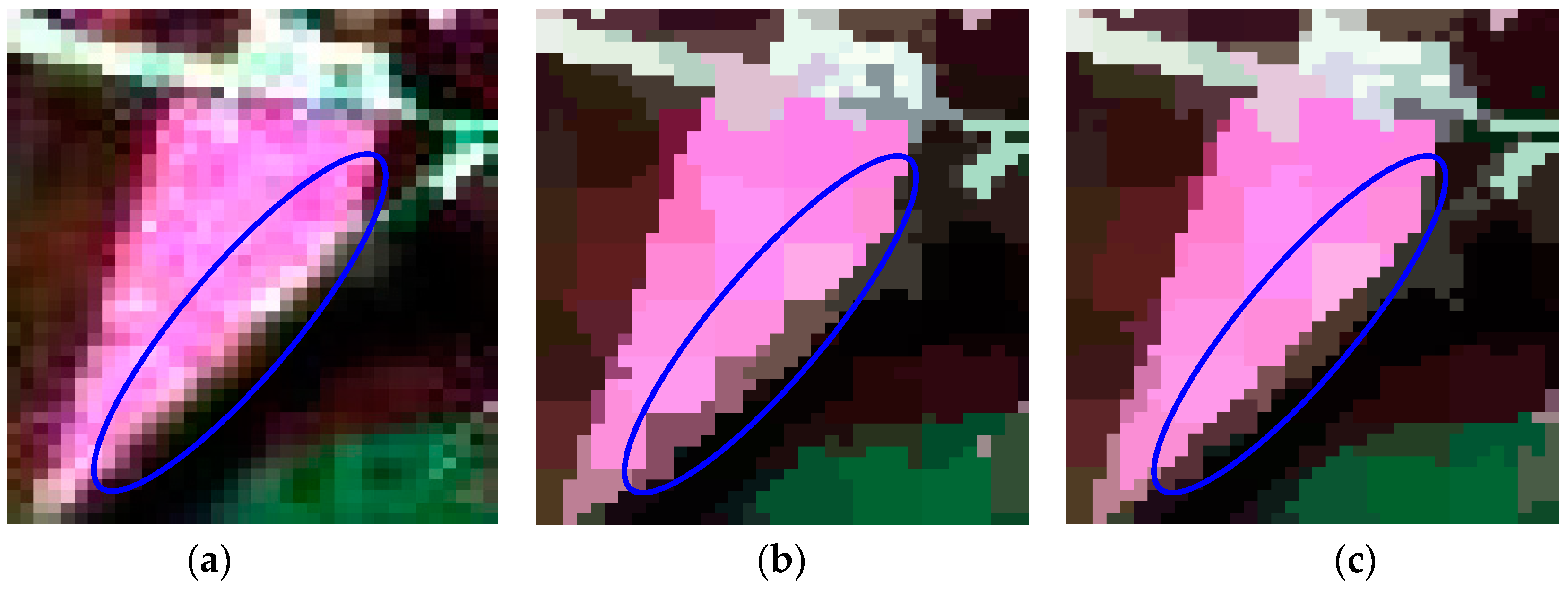
Since the method of our proposed initialization, which initializes the unstable pixels as all the pixels in an image, only showed a slight advantage on the simulated PolSAR data for its large and regular regions, the comparison experiments of two methods of initialization were performed on the first real-world PolSAR image and the results are given in
Figure 7. It can be seen that both methods work well as a whole. Since our method of initialization is proposed for the small or slim regions, we will analyze the details of the results. The details of regions A, B, and C, which are marked in red rectangles in
Figure 7, are compared in
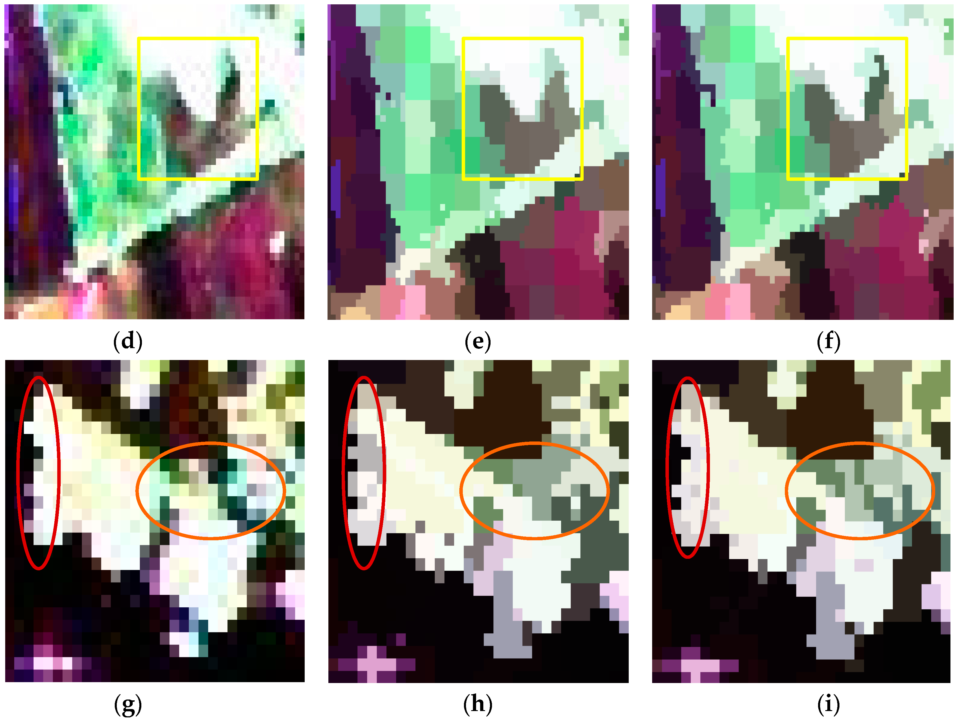
Figure 8. It can be seen from the regions marked by blue ellipses in
Figure 8b,c that our method has a smoother boundary than the GES. That is because our method of initializing unstable pixels contains all the potential edges, however, the GES may lose some edges, especially when the initial grid width is large. The region in the yellow rectangle of
Figure 8f maintains a more similar shape in
Figure 8d than that of
Figure 8e, which also gives the credit to the proposed method of initialization. The last row in
Figure 8 shows that more details are maintained by our method, which indicates that the proposed initialization method can preserve more detail information than the GES. In summary, our proposed method of initialization, compared with the GES, shows the superiority for PolSAR superpixel segmentation.
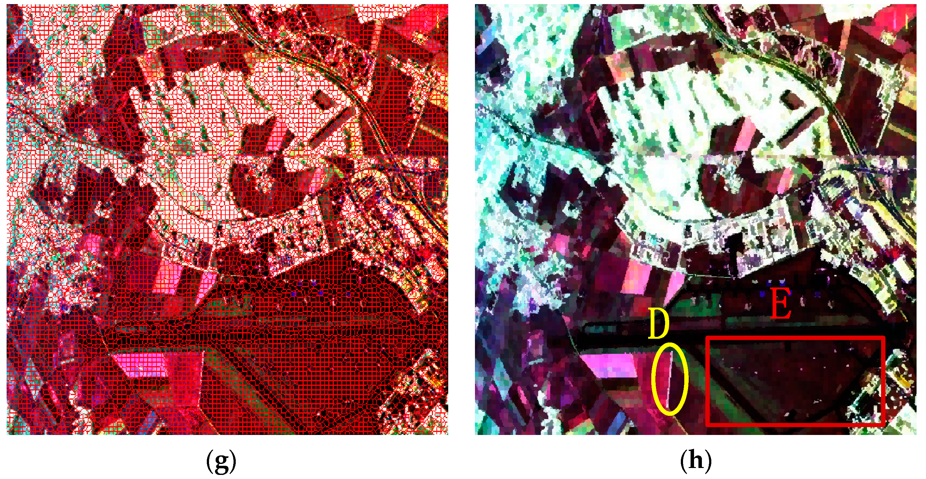
Figure 9 gives the final superpixels of these four methods, in which the standard SLIC, IER, SLIC-GC and Pol-IER are included. The compactness
was set as 15 for the standard SLIC and IER, 0.3 for SLIC-GC and 0.6 for Pol-IER. It can be seen from
Figure 9 that the standard SLIC acquired the worst superpixels. Although its running time, as shown in
Table 1, is the shortest, the generated superpixels’ boundary of the standard SLIC cannot be preserved very well, especially in the slim regions and small regions such as the thin road in the middle of the image and the strong point targets in bottom right regions circled by the red rectangle. The reason is that all the pixels are relabeled according to CIELAB Euclidean distance, which makes more pixels incorrectly labeled. From the first column of
Figure 9, it can be seen that the generated superpixels of IER and Pol-IER are regular in homogeneous areas with good boundary recall, because only unstable pixels rather than all the pixels are relabeled in the step of local relabeling in IER and Pol-IER.
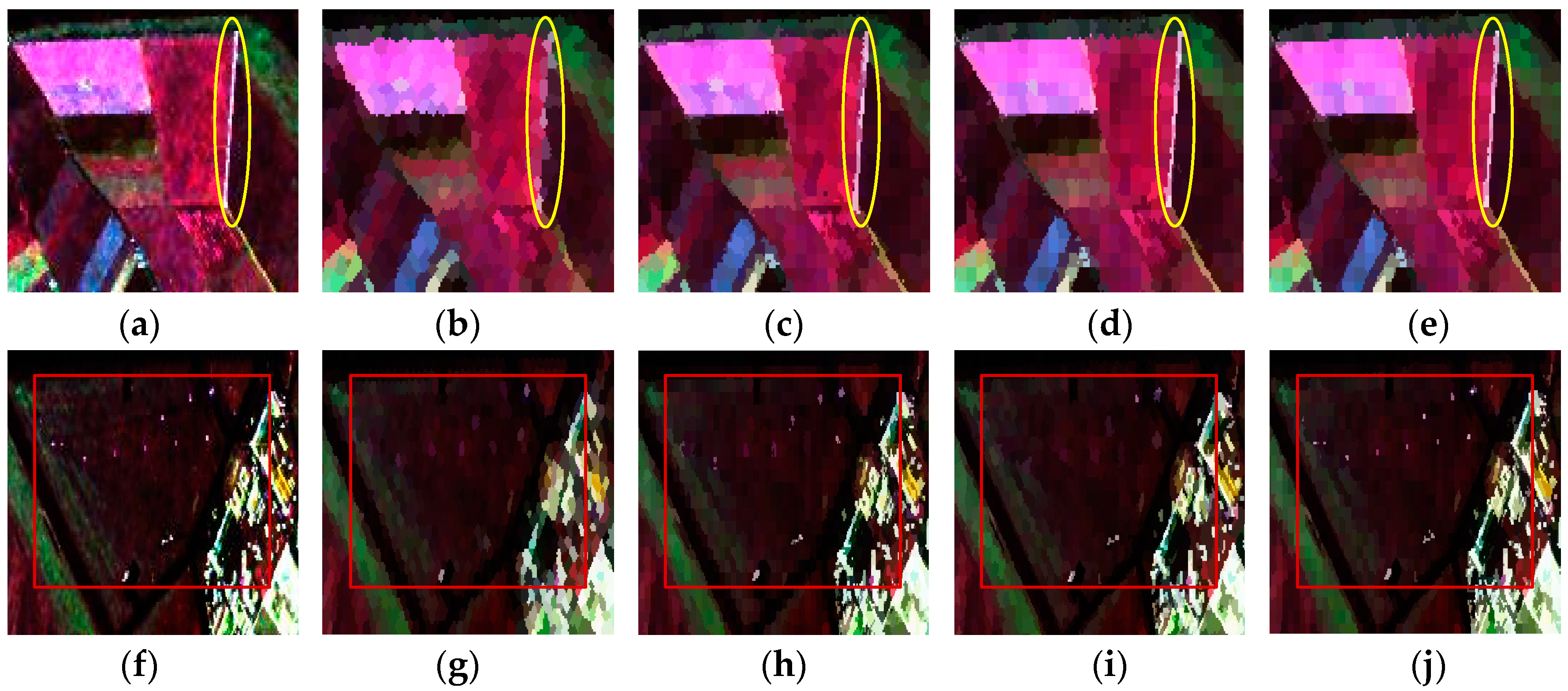
For visual clarity, the small regions D and E in
Figure 9b,d,f,h are enlarged and shown in
Figure 10. From the slim white regions marked by the yellow ellipses in
Figure 10a–e, it can be seen clearly that both SLIC-GC and Pol-IER show good performance in boundary recall, because the revised Wishart distance can better describe the characteristic of PolSAR data than CIELAB Euclidean distance, which means that the coherency matrix provides more information than color for PolSAR images. From the regions marked by red rectangles (in
Figure 10f–j), it can be observed clearly that the strong point targets can be preserved very well by Pol-IER because all the potential edges are maintained and the strong point targets are also preserved by the postprocessing procedure in Pol-IER, while most of the point targets are lost in the other three methods. In summary, Pol-IER performs the best in boundary adherence, regularity and strong point targets preservation.
The running time of these four methods are showed in
Table 1. Since Pol-IER computed the distance based on the coherency matrix instead of the three elements in CIELAB space, the running time of Pol-IER is slightly longer than that of standard SLIC. Besides, only the grid edge pixels are considered as the unstable pixels for IER, while our Pol-IER takes all of the image pixels as unstable pixels in the initialization step, it is reasonable that our Pol-IER is less efficient than the IER. However, as a result of only relabeling unstable pixels, it can be seen that the running time of Pol-IER is more than eight times shorter than the state-of the-art SLIC-GC with the same data distance measure.
4.2.2. Evaluation on the Second Data Set
To further evaluate Pol-IER for real-world PolSAR images, experiments on the second data set were conducted.
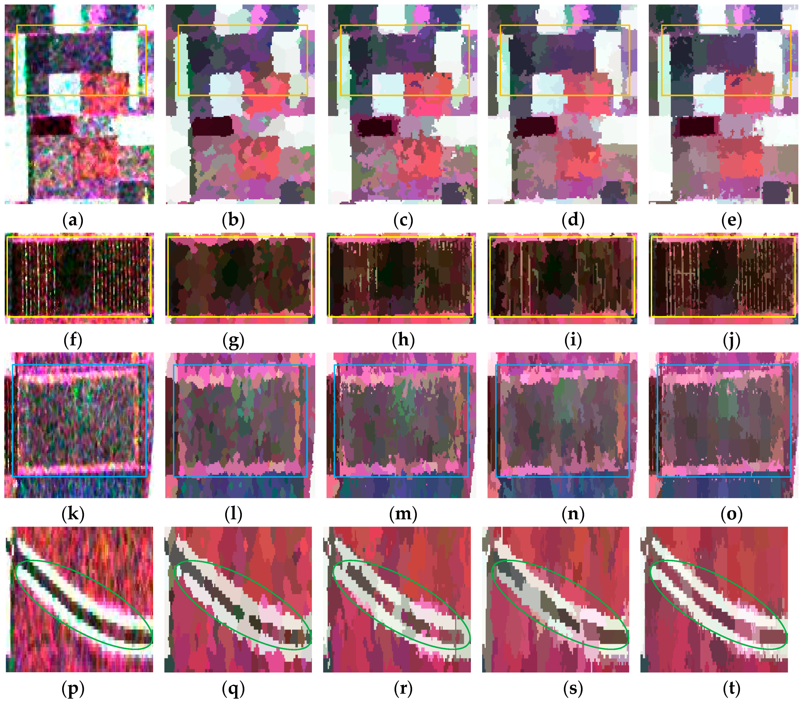
Figure 11 shows the results of the second PolSAR data set by the four algorithms.
Figure 11b–e is the representation maps, where the coherency matrix of each pixel is replaced by the average value of the superpixel to which this pixel belongs. As a whole, it can be seen that the boundary of our method is smoother because of initializing unstable pixels as all the pixels.
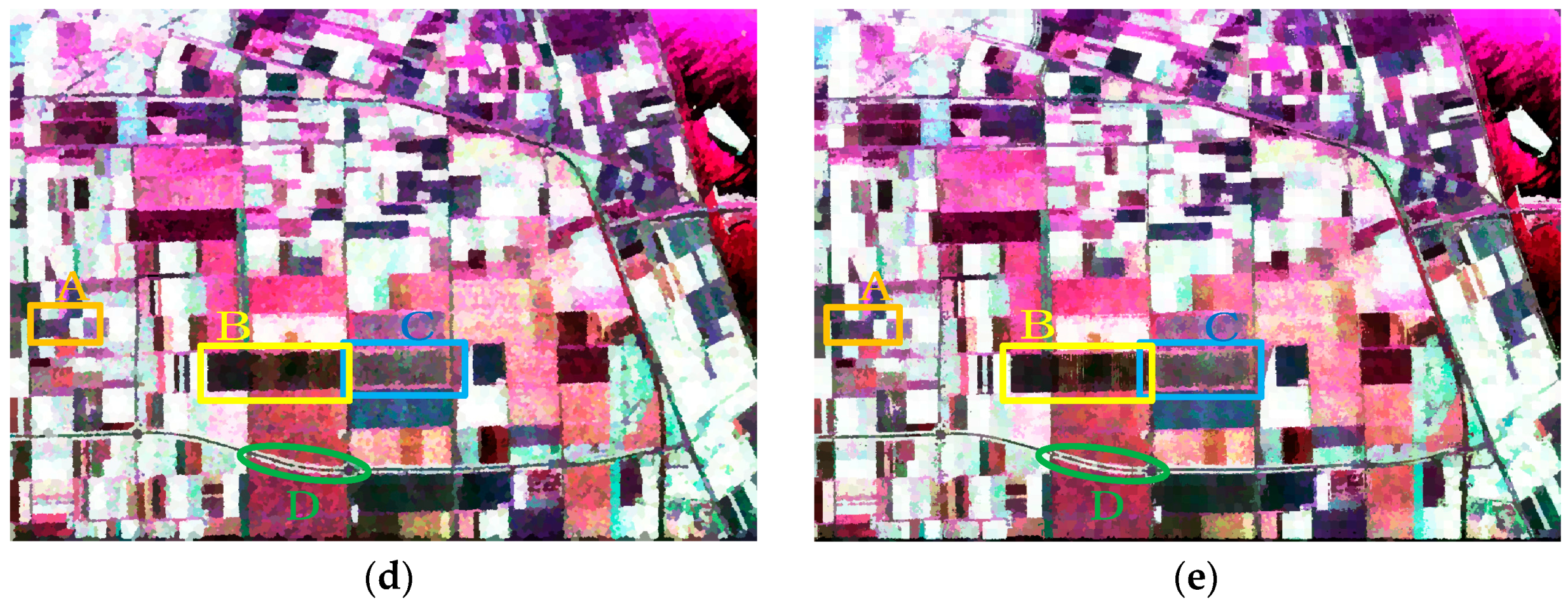
Figure 12 depicts the four patches, i.e., regions A, B, C and D in
Figure 11a–e. Of all the boundaries in region A circled by the orange rectangles in
Figure 12a–e, the last column (
Figure 12e) has the smoothest boundary, which indicates that Pol-IER shows good performance with respect to boundary adherence. From region B in
Figure 12f–j, it can be observed that the boundaries of the slim regions can be preserved best by Pol-IER due to the initialization step and the revised Wishart distance measure. The results of the region C in
Figure 12k–o show that the boundaries generated by Pol-IER are smoother and closer to the real terrain edges. In
Figure 12p–t, it can be seen that only the boundaries of the slim region marked by green ellipses generated by Pol-IER are preserved very well, which demonstrates the superiority of our method in boundary adherence. All the results in
Figure 12 verify that Pol-IER shows good performance in boundary recall. One reason is that the revised Wishart distance can overcome the effect of speckle noise. Another reason is that initializing the unstable pixels as all the pixels and only relabeling unstable pixels can preserve more edges. In addition, the postprocessing procedure removes the small isolated regions as well as preserving strong point targets.
Table 2 is the running time of these four methods. It can be seen that the running time of Pol-IER is about nine times shorter than that of SLIC-GC as a result of only relabeling unstable pixels.
In summary, the proposed method shows better performance than standard SLIC and IER, which is because the revised Wishart distance between two coherency matrices can better describe the data distance than the Euclidean distance in CIELAB color space, and the postprocessing based on a dissimilarity measure can better preserve the strong point targets than CCA. Our algorithm outperforms SLIC-GC as a result of initializing unstable pixels as all the pixels, which makes all the potential edges contained; only relabeling unstable pixels, which makes the proposed method more efficient and avoids incorrectly sorting more pixels; and implementing the revised Wishart distance in a fast way, which makes the computation efficiency further higher.
5. Conclusions
IER is a fast superpixel segmentation algorithm for optical images. Due to the inherent speckle noise and the existence of many small-sized or slim regions in PolSAR images, a fast PolSAR superpixel segmentation based on edge refinement and fast revised Wishart distance was proposed in this paper. The fast revised Wishart distance between two coherency matrices was utilized in the local relabeling of the unstable pixels instead of Euclidean distance in CIELAB color space to reduce the impact of speckle noise. To preserve the edges of the small-sized and slim regions as much as possible, the initialization of unstable pixels was set as all the pixels in PolSAR images rather than only the grid edge pixels. Finally, a postprocessing procedure, based on the dissimilarity measure, was employed to remove the generated small isolated regions as well as to preserve the strong point targets. The evaluations on four simulated PolSAR images with different sizes demonstrated the availability of the fast revised Wishart distance and the proposed initialization in terms of four commonly used criteria, i.e., BR, USE, ASA and running time. The experiments on two real-world PolSAR images showed that our proposed Pol-IER outperformed the other three methods including standard SLIC, IER and SLIC-GC in boundary adherence, regularity and strong point targets’ preservation. Although the running time is slightly longer than the standard SLIC and IER, it is much shorter compared with other methods of superpixel generation for PolSAR images and is even about nine times shorter than that of SLIC-GC with large-sized images. However, as a result of initializing all the image pixels as unstable pixels, the Pol-IER is more time consuming compared to the standard SLIC and IER which are originally proposed to generate superpixels for optical images. Therefore, it would be beneficial to further improve the efficiency of our proposed approach in future work.


