1. Introduction
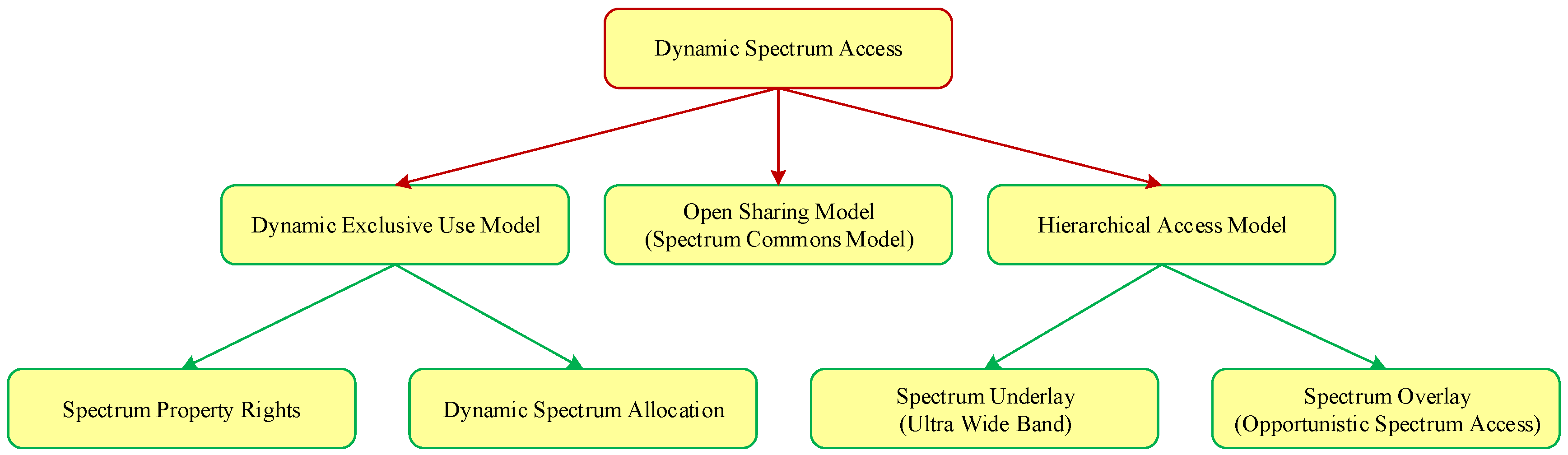
Cognitive radio (CR) is a promising technology which can fully use the spectrum by dynamically accessing the primary network. Consequently, dynamic spectrum access technology plays a very significant role and has become a hot research topic. As illustrated in
Figure 1, dynamic spectrum access strategies can be classified into three models, e.g., the dynamic exclusive use model, the open sharing model, and the hierarchical model. Among those models, the hierarchical model is a hierarchical access structure for primary users (PUs) and secondary users (SUs), and is the most promising and effective one for current spectrum access policies [
1]. The basic idea of the hierarchical model is that the SUs can use the licensed spectrum of PUs, as long as they can limit any interference perceived by PUs. Furthermore, there are two models of the spectrum sharing between PUs and SUs, namely spectrum underlay and spectrum overlay.
Spectrum underlay introduces severe constraints on the transmission power of the SUs, therefore, it spreads the transmitted signals over a wide frequency band. The SUs can achieve low data rates with very low transmission power. If the PUs transmit in all the time-slots, the spectrum underlay does not need to detect and perceive the spectrum of the PUs.
Spectrum overlay, first presented by Mitola, can be also regarded as opportunistic spectrum access (OSA). Compared to the spectrum underlay, this model needs to detect and perceive the spectra of the PUs. It finds spatial and temporal spectrum white space for SUs to use, which is also termed as the spectrum holes (SHs). Therefore, this model does not need to obey the severe transmission power constraints of the SUs, and the SUs can achieve high date rates with high transmission power.
In most cases, the spectrum overlay and underlay models are used separately. In this paper, a hybrid spectrum access model is proposed to use both the overlay and underlay methods simultaneously to further improve the current spectrum efficiency.
The spectrum hole (SH) is a part of the licensed spectrum which is not being used by the owner during a period of time [
1]. Among key technologies in CR, the design of the control channel is essential because the SUs need a control channel to coordinate and they have no licensed spectrum to carry the control information. The vulnerabilities resulting from utilizing a dedicated control channel have been well studied. Existing studies of the control channel have shown that using SHs to convey control information is only a basic approach and many shortcomings have been pointed out [
2,
3,
4,
5,
6]. Firstly, the SUs may not have a common SH as control channel which would lead to low connectivity of the SUs. Secondly, the arrival of PU is unknown which causes interruptions in the use of the control channel.
As the SUs communicate only in the SHs, the SUs need information about those unused bands in which the PUs are inactive. Each SU should maintain a list of SHs which probably will differ from one to another. The SUs can communicate with each other if there is a common SH in their lists. Consequently, there should be a way to pass information about the lists between SUs during the initial communication.
Most of the existing MAC protocols of CR sensor networks are focused on avoiding common control channels. However, in this paper, a new method of spreading the power spectrum density in a control channel over an ultra-wide bandwidth is proposed to exploit the underused (gray) spectral regions. Like underlay spectrum sharing, the SUs can always access to the spectrum as long as the interference causing by SUs at the PU receiver can satisfactorily meet the threshold constraint [
7].
According to the above analysis and considering the low power spectrum density of underlay waveforms, we propose to design a control channel to convey a small amount of control information, which is termed as SUCCH. At the same time, the spectrum overlay waveform is adopted to exchange a large amount of date, which is named as SUTCH. Our study is based on a spectrum sharing system consisting of two different waveforms. The first one is the Direct Sequence Code Division Multiple Access (DS-CDMA), which is defined as the underlay waveform used to convey control information. The second one is the Non-Contiguous Orthogonal Frequency Division Multiplexing (NC-OFDM), which is defined as the overlay waveform used to convey data information. The spectrum of NC-OFDM-based SUs is shared with the PUs which utilize DS-CDMA. Spreading Gain of DS-CDMA provides the required anti-jamming capability for the interference which may be caused by the SUs. In the meantime, based on the properties of the non-continuous power spectrum of NC-OFDM, it is more flexible for the SUs to access the SHs which are discontinuous in the frequency spectrum [
8]. It is of great significance to discuss and study this issue, since the existing DS-CDMA is anticipated to be one of the spectrum sharing applications used in the future [
9].
In order to set up the hybrid spectrum access model, several questions should be answered. The first one is the procedure for network setup between two SUs. The second one is the maximum access capacity of the SUTCH with different strategies. The third one is the reliability of the SUCCH. The fourth one is the power allocation strategies of the SUs between the SUTCH and SUCCH. In the rest of this paper, the above questions will be answered in detail. Specifically,
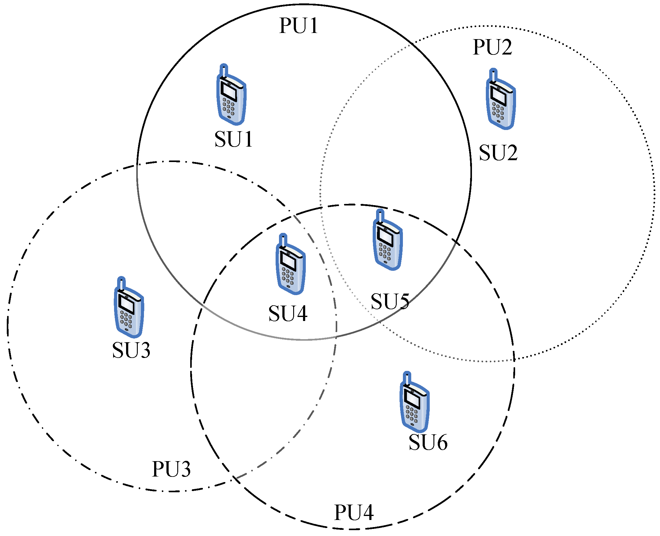
Section 2 builds application scenarios and proposes a mechanism for establishing the CR sensor networks. In
Section 3, a transmission channel model for analyzing the maximum access capacity for different polices with different objectives in the fading environment will be discussed. In
Section 4, the reliability of the SUCCH is analyzed, and a hybrid spectrum access algorithm based on reinforcement learning model is proposed for the power allocation problem of the SUTCH and the SUCCH. Finally,
Section 5 presents our simulation results and
Section 6 concludes the paper.
3. Subchannel Selection Policies
Suppose the wireless channel is a frequency-selective Additive White Gaussian Noise (AWGN), the bandwidth is B Hz, and the power spectral density is N0. In this paper, it is divided into N Rayleigh fading subchannels, and the subchannel coherence bandwidth is ∆f Hz. Therefore, B = N∆f. These subchannels are indexed by i = 1, 2, …, N, and the gains of every subchannel are independent and identically distributed (i.i.d).
Active PUs use DS-CDMA technology to access the spectrum band with spreading gain
G. According to the Central Limit Theorem, the interference process in the receiver of the SUs caused by a large number of PUs is considered a Gaussian approximation. Furthermore, according to the second-order statistics, the interference process is a white process [
14]. Therefore, in each subchannel, the average interference introduced by the PUs at the receiver of the SUs is (
K − 1)
N0∆
f,
K ≥ 1, where
K is a system parameter related to the characteristics of PUs network [
15].
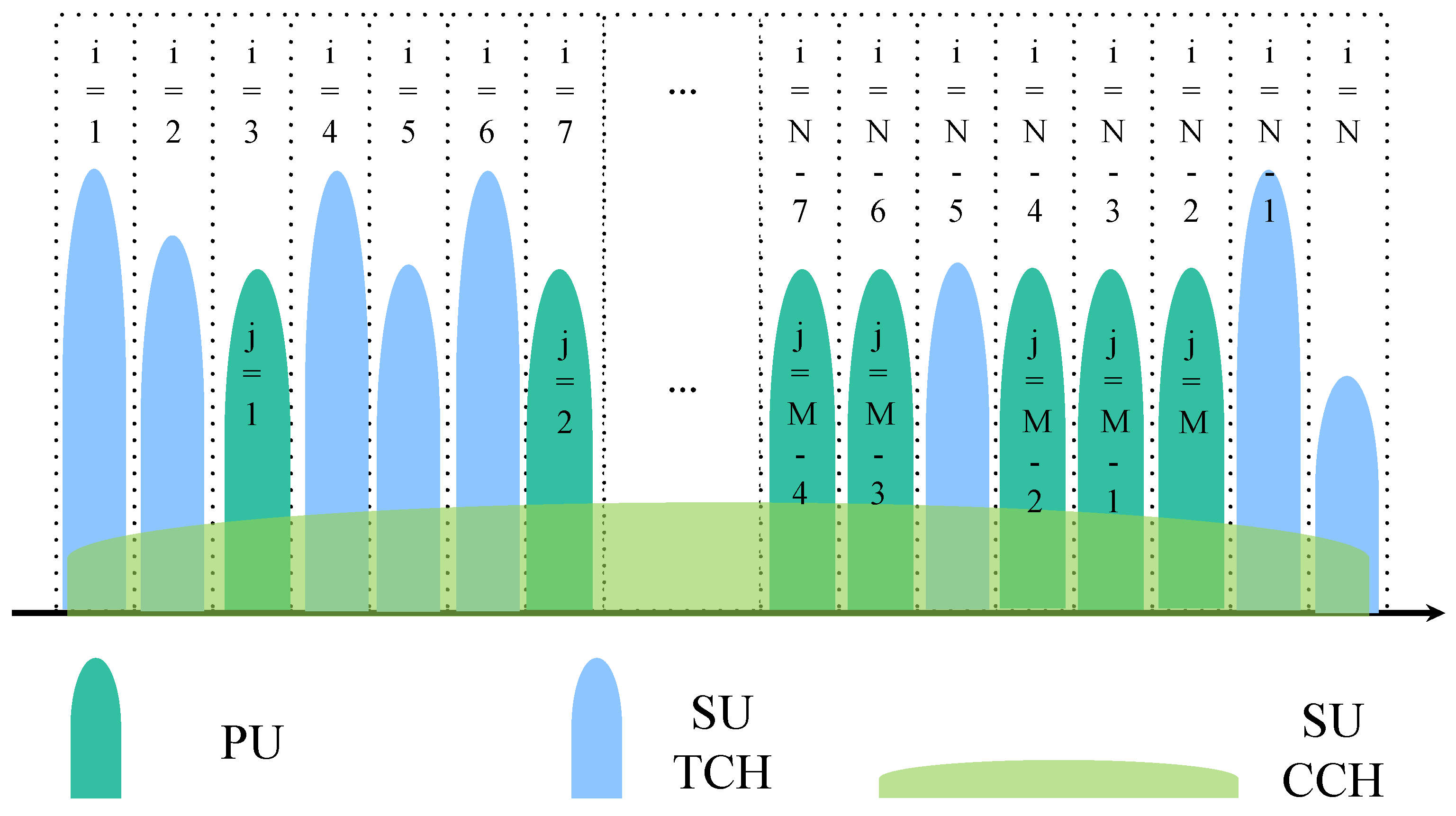
As shown in
Figure 4, the SUs utilize NC-OFDM to access the SUTCH which is indexed by
j = 1, 2, …,
M, 0 ≤
M ≤
N. The SUs spread their SUCCH power spectrum density over an ultra-wide bandwidth to exploit the underused (gray) spectral.
Q is defined as the interference threshold of the PUs, which is the maximum allowable temporal interference in the receiver of the PUs caused by concurrent activity of the SUs in the same subchannel. As mentioned in
Figure 4, the protocol to set up CR sensor networks is based on the time-slot structure. Therefore, in order to satisfy the interference threshold constraint, the power of the SUs accessing the SUTCH should be controlled in each time-slot.
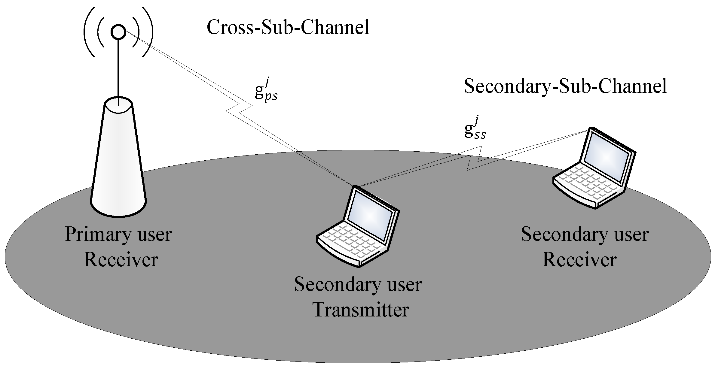
In this paper, the structure of the accessing system is depicted in
Figure 5. For subchannel
j, the instantaneous gain between the transmitter and receiver of the SU is defined as
, and the instantaneous gain between the transmitter of the SU and the receiver of the PU is defined as
. Subscripts
s and
p refer to the secondary and the primary user, respectively. The
and
are assumed as the stationary and ergodic independent distributed random variables with unit-mean. Their Probability Density Functions (PDFs) are defined as
and
, respectively. Channel gains
and
are i.i.d.,
j = 1, 2, …,
M. In this paper, we suppose the perfect Channel Side Information (CSI) pair (
can be available in the transmitters. Here, the CSI contains the probability distribution of the channel gain, as well as the actual value at a certain time-slot. Actually, the CSI pair can be estimated by a spectral coordinator or proper signaling. Note that, the result derived from this assumption is an upper-bound in the case without a perfect CSI pair.
In this paper, we focus on the maximum achievable spectrum capacity of SUTCH, which is studied [
16,
17]. Since more than one SUs will compete to access to the underused frequency band. The SUs’ total available spectrum capacity is upper-bound by the case of only one SU, which is due to the fact that SUs will impose interference on each other. Therefore, the discussion of the individual SU can also be used as the upper-bound of the total spectrum capacity of all SUs.
At a given time-slot, the power allocation policy of SUTCH is defined as
, which is based on a selection criterion
ψ(,..,), and set:
For the observing random variables
μj,
j = 1, …,
M, the selection sequence
γM is defined as follows:
The M-tuple selection sequence is arranged, so that its first element is the most suitable subchannel for SUTCH based on the selection criteria in Equation (1). The probability distribution function of random variable γj is defined as kj(γ), j = 1, …, M. It is important to note that if j1, j2 are entities in γM and j1 < j2, then it can be considered that compared to the choice j2, the SUs can get a better performance by choosing subchannel with index j1.
Suppose is constant, which means subchannels are considered equally. The SUs will randomly choose M out of N subchannels without any a priori information. This selection strategy is defined as the uniform subchannel selection, whereas, if the prior information of the subchannel obtained by cooperation or other techniques is −1, the SUs will choose the corresponding value of . This selection strategy is defined as the non-uniform selection strategy.
The transmission power of the SUTCH in the subchannel
j is referred to
Psj.
Ps(
Ps1, …,
PsM) is defined as the transmission power vector of SUTCH over
M subchannels. Suppose that SUTCH accesses to the chosen subchannel
j with the transmission power of
Psj, and the corresponding interference at the receiver of the PUs is
Qj, where:
Since the PUs utilize DS-CDMA with spreading gain
G, therefore, the narrow-band interference
Qj spreads over the whole bandwidth and manifests itself as an equivalent wide-band interference equal to
G−1Qj at the receiver of the PUs. Suppose the SUTCH transmits with the transmission power vector
Ps(
Ps1,
Ps2, …,
PsM) in
M accessible subchannels. Correspondingly, an equivalent narrow-band interference vector
Q = (
Q1,
Q2, …,
QM) will be imposed on the receivers of the PUs. Meanwhile, the SUCCH transmits with the transmission power vector
Psc(
Psc1,
Psc2, …,
PscN). Therefore, in order to comply with the interference threshold
Q of the PUs, the constraint function is as follows:
In this paper, the objective is to achieve the maximum capacity of SUTCH. As discussed above, the transmitting power of SUTCH in each accessible subchannel should be optimally allocated. Meantime, the interference threshold constraint should also be considered. Consequently, according to selection policy
, for a given
Q and for
M accessible subchannels, the maximum capacity of SUTCH is defined as
, which can be obtained by the following constrained optimization problem:
where,
Q is the interference threshold of the PUs, which is the maximum allowable temporal interference in the receiver of the PUs caused by concurrent activity of the SUs in the same subchannel.
Ps N0 is the power spectral density, ∆
f is the subchannel coherence bandwidth.
K is a system parameter related to the characteristics of PUs network [
15] within the range of 2–8. Equation (5) is derived from Shannon’s Capacity formula with the SUs power vector
Ps and
Psc. Equation (6) is the constraint function of interference threshold of the PUs and maximum transmitting power of the SUs.
Actually, in contrast to the constraint of maximum transmitting power of the SUs, the constraint function of interference threshold of the PUs is much tighter [
18]. Therefore, in this paper, the constraint of maximum transmitting power of SUs is not considered. At the same time, as mentioned above, the SUCCH spreads over an ultra-wide bandwidth to exploit the underused spectrum with a very low PSD, therefore, the interference caused by SUCCH is very low. In this paper, in order to simplify the analysis, the effect of SUCCH will not be considered, and Equation (5) will be further simplified as follows:
Suppose
= 1, thus the SUs will randomly choose
M out of
N subchannels without any priori information by
ρ1, which is a uniform subchannel selection policy. Consequently, substituting
and defining
Equation (6) can be simplified as follows:
where
0 ≤
vj ≤ ∞,
is the reward factor of the subchannel
j.
is defined as the spectrum sharing load factor of the subchannel
j.
Suppose the statistics characteristics of
is i.i.d. Rayleigh random variables,
and
are exponentially distributed random variables with unit-mean, therefore, the PDF of
can be converted into [
17]:
Substituting Equation (9) into Equation (7), and integrating by part, Equation (10) can be gotten as follows, which is the simplified optimization problem of
:
where,
is defined as the spectrum sharing load factor, and
is defined as the spectrum sharing load vector:
Furthermore, the following pseudo linear approximation is used to get an approximate solution for Equation (10) [
16]:
Substituting Equation (12) into Equation (10), the Lagrangian function of the optimization problem Equation (10) is shown as follows [
19,
20]:
where
λ is the Lagrangian coefficient. The derivative with respect to the
on Equation (13) is taken, and then it is equal to zero, the following formula can be obtained:
Substituting Equation (14) into Equation (10), the following formula can obtained:
Equivalently, Equation (16) can be derived from Equation (15):
Eventually, substituting Equation (16) into Equation (14) gives:
Note that Equation (17) suggests that for given
G,
N,
M and
θQ, the maximum capacity is achieved by dividing the total acceptable interference
GNθQ into equal portions for
M accessible subchannels. Actually, it is a direct consequence of selecting
M out of
N subchannels without any prior knowledge. Furthermore, according to Equation (3) and
, the optimal transmitting power vector
can be obtained as follows:
Equation (18) suggests that the interference share for each accessible subchannel j, is mapped to the corresponding transmission power Psj, proportional to 1/. So, if is large, then the SUs will creates a large interference in the receivers of Pus. In this case, Equation (18) suggests a lower SUs transmission power in accessible subchannel j.
Equivalently, substituting Equation (18) into Equation (10), Equation (19) can be derived:
In a practical case, Q = G−1N0B and M < N, the spectrum sharing load factor can be obtained from Equation (17) as , which is much higher than unity.
As mentioned above, randomly choose subchannels, which ignores the fact that it is more reasonable for the SUs to allocate higher transmission power to certain subchannels because of their corresponding CSIs, so it is essential to discuss the non-uniform selection policy for SUTCH with a prior knowledge of CSIs pair (, ), since it will lead to a larger capacity or a smaller interference on the PUs.
Actually, an appropriate selection policy should consider the interference of the PUs receivers caused by SUs transmission. Such policy should select the lower subchannel gain of , because it will create a lower interference in the receivers of the PUs. Therefore, a lower will give the SUs the flexibility of allocating a higher power, which will result in a higher capacity. Such a selection policy is named as SU-PU-based selection policy, which is simplified as . In order to implement , the SUs requires during each time-slot. Therefore, a signaling channel between the receivers of the PUs and the transmitters of the SUs is required.
Similar to , another selection policy can be derived. It will select those subchannels which achieve the highest capacity corresponding to allocating the transmitting power of SUs. Such policy selects the subchannel with the higher , because it will create a higher power in the receivers of the SUs. Such selection is name as SU-SU-based selection policy, which is simplified as . In order to implement , the SUs requires during each time-slot. Therefore, a signaling channel between the receivers of the SUs and the transmitters of the SUs is also required. In the following, the maximum capacity is derived with different selection policy and .
Considering
, the selection criteria can be assumed as follows:
Consequently,
and based on
μj,
j = 1, 2, …,
M, the selection sequence is defined as follows:
where
μ1 ≤
μ1 ≤ … ≤
μM. Using order statistics [
21], the probability distribution function of
μj, ∀
j is shown as follows:
where:
and
fμ(
μ),
Fμ(
μ) are the probability density function and probability distribution function of
μ. Assuming the same assumption as discussed above in Equation (9) we obtain:
Using a binomial expansion to replace (1 −
e−μ)
j−1 in Equation (25) gives:
where,
.
Thus, the optimization problem of maximizing the capacity of SUTCH, while satisfying the tolerable interference constraint of the PUs with selection policy
is shown as follows:
However, in practice,
M <
N, thus,
. Therefore, Equation (27) can be approximated by Equation (28):
The Lagrange multiplier algorithm can be used to solve the optimization problem in Equation (28) [
19]:
where,
λ is the Lagrangian coefficient.
Taking the derivative with respect to the
on Equation (29) and setting it equal to zero gives:
where,
. Substituting Equation (30) into Equation (28):
Substituting Equation (31) into Equation (30):
Furthermore, according to Equation (3) and
, the optimal transmitting power vector
with selection policy
can be obtained as follows:
Equivalently, substituting Equation (33) into Equation (28) yields the approximated maximum achievable capacity of the SUTCH with selection policy
, which is shown in Equation (34):
Considering
, the selection criteria can be assumed as follows:
Consequently,
and based on
μj,
j = 1, 2, …,
M, the selection sequence is defined as follows:
where
μ1 ≥
μ2 ≥ … ≥
μM. Using order statistics [
21], the probability distribution function of
μj, ∀
j is shown as follows:
Using a binomial expansion to replace (1 −
e−μ)
N−j in Equation (37) one obtains:
where
.
Thus the optimization problem of maximizing the capacity of the SUTCH while satisfying the tolerable interference constraints of the PUs with selection policy
is shown as follows:
Utilizing the following approximation for small values of
l = 0, 1, …,
N − j as:
where:
Furthermore, according to Equation (3) and
, the optimal transmitting power vector
with selection policy
can be achieved as follows:
Equivalently, substituting (41) into (39) yields the approximated maximum achievable capacity of the SUTCH under SU-SU-based selection policy is shown as follows:
4. Reinforcement Learning for Improving Performance
In
Section 3, the maximum achievable capacity of the SUTCH is analyzed. In
Section 4, the reliability of the SUCCH is taken into consideration by the Bit Error Rate (BER). Suppose the signal waveform of the SUCCH is as follows:
Suppose the two signal waveforms in Equation (45) are transmitted with the same probability. Since the SUCCH spreads its power spectrum density over an ultra-wide bandwidth to exploit the underused (gray) spectral regions, the interference process caused by the PUs and the SUCCH can be considered as a Gaussian approximation. If the SUCCH transmits
s1(
t), after the despread-demodulation algorithm at the receiver of the SUCCH, the received signal is as follows:
where
n is additive Gaussian white noise with mean zero, variance
N0/2 and
σPU,
σSUCCH represent the interference caused by the PUs and the SUTCH.
GSUCCH is the spreading gain of the SUCCH. The receiving signal of the SUCCH is compared with the threshold zero, which is as follows:
Suppose the PUs and the SUCCH are i.i.d. random processes, then two probability density functions of
r are given as follows:
Consequently, the average error probability of the SUCCH is as follows:
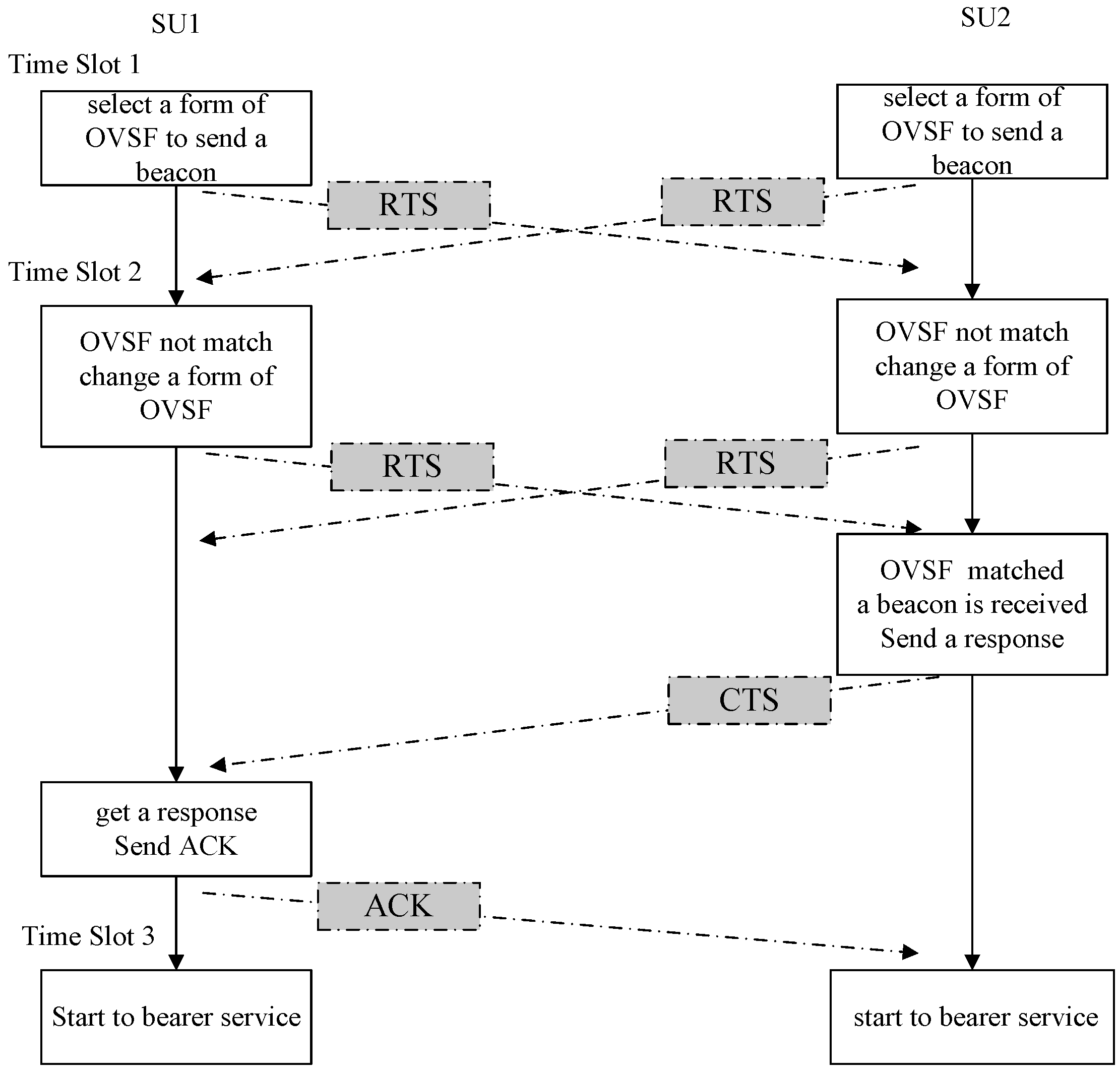
Suppose the control information of the SUCCH consists of 8 bits. According to
Figure 4, the transmitter and receiver of the SUs need to coordinate access to the spectrum three times. Therefore, the probability of successful establishment for the SUCCH can be concluded. Furthermore, the total interference caused by the SUs is divided into two parts:
QSUTCH and
QSUCCH.
QSUTCH represents the interference caused by the activity of the SUTCH, while
QSUCCH represents the interference caused by the activity of the SUTCH. The loading factor Г is defined as the radio of
QSUTCH and
QSUCCH, which is as follows:
In consideration of the link access protocol design described above and the probability of successful establishment for SUCCH, the lower PSD of SUCCH means it may take more time to complete the setup procedure for the SUs. In other words, accessible subchannels will remain idle for a long period of time, which will lead to spectrum resource waste. However, increasing the transmitting power of the SUCCH will decrease the transmitting power of the SUTCH, because of the total interference constraint caused by the SUs is certain at a time-slot. Lower transmitting power of the SUTCH will lead to reduce the capacity of data. Therefore, it’s a trade-off, which is essential to choose the appropriate transmitting power of SUTCH according to the characteristic of the activity of the PU. For this purpose, a hybrid access method based on Reinforcement Learning model is proposed to solve this problem. The most prominent feature of Reinforcement Learning model is its autonomous learning and online learning ability. By trial and error, Reinforcement Learning model can get a better strategy based on the subchannel environment.
The Cross model [
22] is now widely recognized as one of the Reinforcement Learning models with memory-less characteristics, which means the learning process is a Markov Decision Process (MDP). The basic idea is to follow the rules of “Results” [
23], namely, if system is rewarded by choosing a strategy, then the next period will get higher probability of choosing such strategy. On the contrary, if it is punished, the next period will reduce the probability of choosing such strategy.
Bush and Mosteller [
24] introduced the Bush-Mosteller model in 1955 [
25]. Afterwards, Roth and Erev improved this model and introduced the Roth-Ever model. Nowadays, as two models of reinforcement learning, both of them [
26] are widely adopted. They are easy to realize and have very low computation complexity, which fit for the real-time applications. Therefore, in this paper, these two models are introduced and some necessary modifications are adopted for the application, so the model of MDP Cross and Statistical Mean are proposed.
As mentioned above, the process of connection setup is defined as the time-slotted. The optional strategies for the SUs are defined as follows:
where
Asu is the vector of optional strategies,
R the number of the strategy,
n is the chosen strategy and
n′ are not chosen strategies in a certain time-slot.
Consequently, during the time-slot
k to access the initial stage, the SUs can update the probability of choosing strategy
n and
n′ by the following formula:
where
Asu(
k) is the accessible strategy of the SUs at the time-slot
k, which can be seen the action of MDP.
pn(
k) is the probability of the accessible strategy
n of the SUs at time-slot
k,
pn(
k) is the probability of the unused strategy
n′ of the SUs at time-slot
k, which can be seen as the state of MDP.
u(
k) is the reward function of the accessible performance of the SUs, which can be seen as the reward of MDP.
α and
β are the adjustment factors, which can be used to determine the updating rate of
u(
k).
R[
u(
k)] is defined as the monotone function of
u(
k), which is −1 <
R[
u(
k)] < 1. When the SUTCH successfully accesses idle subchannels, it obtains the reward, which is defined as follows:
where,
T(
k) is the transmission duration of the SUs in time-slot
k and ∂
1 is a weighting factor and
I(
k) is indicator function, which is defined as follows:
When the SUTCH fails to access the idle subchannels, it wastes the opportunity for transmission and pays the cost, which is shown as follows:
where,
T′(
k) is the access duration of the SUs and ∂
2 is also a weighting factor.
In order to weaken the impact of weighting on updating the probability of the choosing strategy, Equation (52) can be further defined as follows:
where,
ε =
R[
u(
k)] =
α ×
u(
k)+
β. The solution to update the probability of choosing strategy is the model of MDP Cross. If the
u(
k) > 0, which means the accessible strategy
n is fit for the current subchannel environment. Therefore, the
pn(
k + 1) should be increased, while the
pn′ (
k + 1) should be decreased. However, if the
u(
k) < 0, which means the accessible strategy
n is not fit for the current subchannel environment, therefore, the
pn(
k + 1) should be decreased, while the
pn′(
k + 1) should be increased.
In practice, the probability of choosing a strategy is usually not only dependent on the latest result, it also takes the “system history” into account. “System history” presents users with more information about the status of environment. In order to incorporate the “system history”, the Statistical Mean is proposed, in which the reward function is modified as follows:
where,
represents the amount of data traffic which SUTCH has transmitted based on strategy
n at time-slot
k,
and
are the idea and wasted amount, respectively.
Therefore the probability of choosing a strategy in the Statistical Mean is shown as follows:
5. Simulation Study
In this section, the achievable spectrum efficiencies with different subchannel selection policies are compared. Here, the spectrum sharing load factor is
θQ = −30 dB and the number of subchannels is
N = 40. The mean values of random variables
are denoted by
, respectively. The achieved spectrum efficiency is defined as follows:
Here, in order to facilitate the comparison, is defined as the achieved spectrum efficiency with uniform subchannel selection, is defined as the achieved spectrum efficiency with the SU-SU-based selection policy, is defined as the achieved spectrum efficiency with the SU-PU-based selection policy.
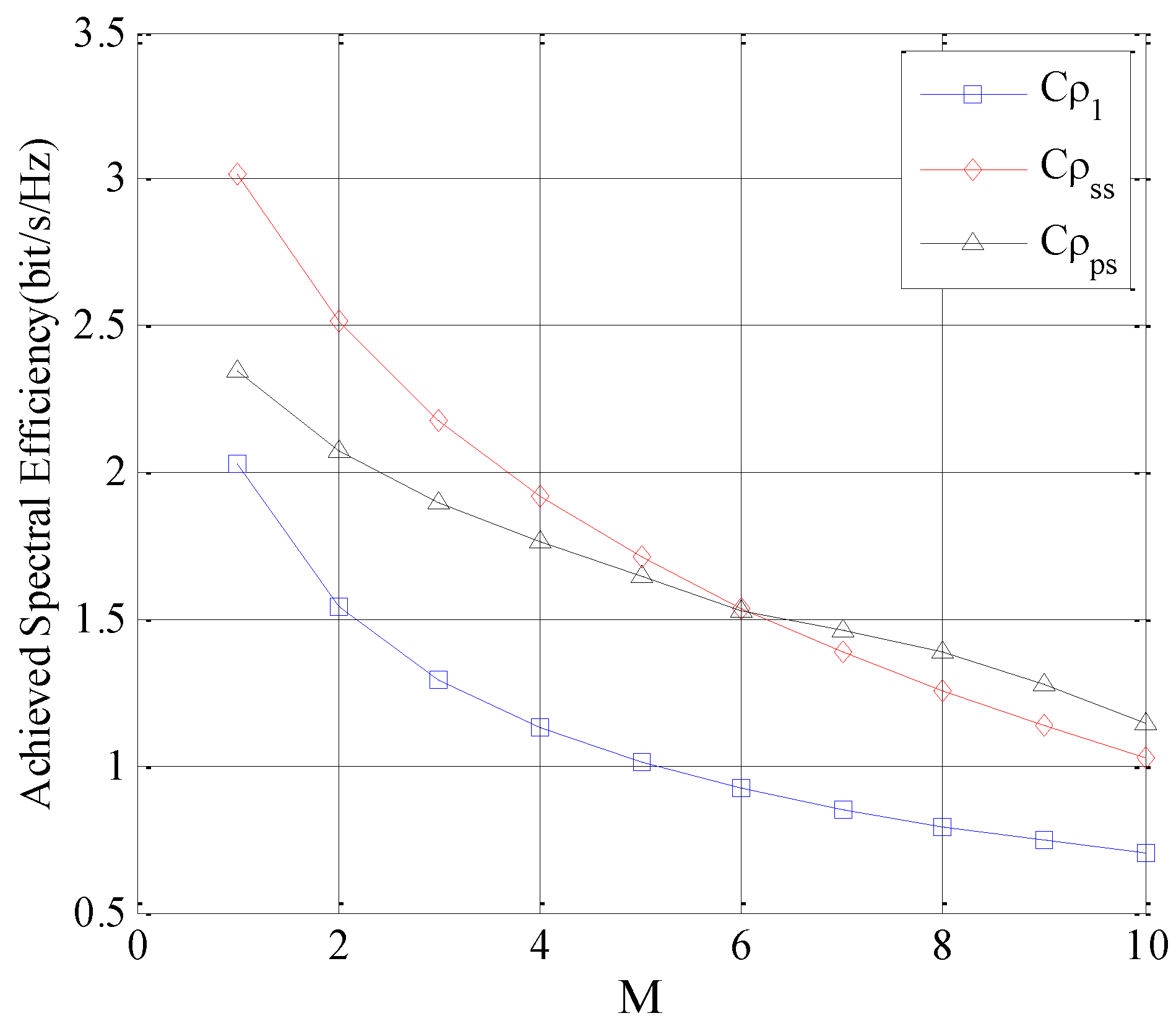
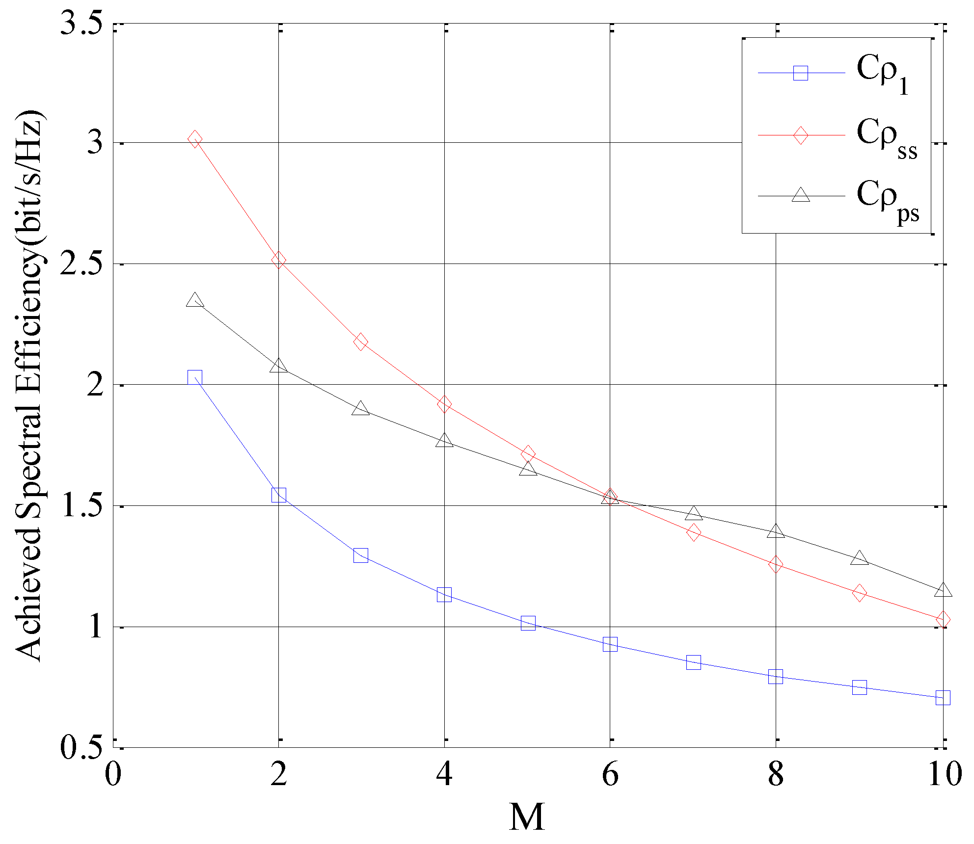
In the first simulation, suppose the interference threshold is a constant and
, and the
is analyzed by increasing
M, which is depicted in
Figure 6.
As depicted in
Figure 6,
is lower than that of
and
, therefore, it indicates that
ρ1 has a poorer performance compared to
ρss and
ρps. For
M = 1, the gap between
and
is large. However, with the increase of
M, the gap is reduced. This result is reasonable because the tap is related to the
M/
N ratio, and the larger
M/
N, the lower the tap is. The reason is that for a larger
M/
N, the set of
M subchannels accessible by
and
probably has a large overlap.
With the increase of
M, the rate of decrease of
ρps is reduced with the slowest rate. This is mainly due to the fact that the total interference threshold of the receivers of the PUs is a constant. At the same time,
ρps selects these subchannels with the lower
, which enables the SUs transmitters to send the maximum transmitting power, without generating high interference on the receivers of the Pus and satisfying the constraint of the interference threshold of the PUs. According to
Figure 6, for a large number of accessible subchannels with constant interference constraint,
ρps achieves a better performance.
In the second simulation, the influence of the number of subchannels
N is analyzed. Suppose
M = 1,
, the
is analyzed by increasing
N. The result is depicted in
Figure 7.
As seen in
Figure 7, for all the different subchannel selection policies, the
increases with the increase of
N. This is because that the probability of selecting proper subchannels for SUTCH is increasing with
N. Furthermore, it is interesting to find that the gap between these three selection policies also increases with the increase of
N and
ρss outperforms the others in this simulation.
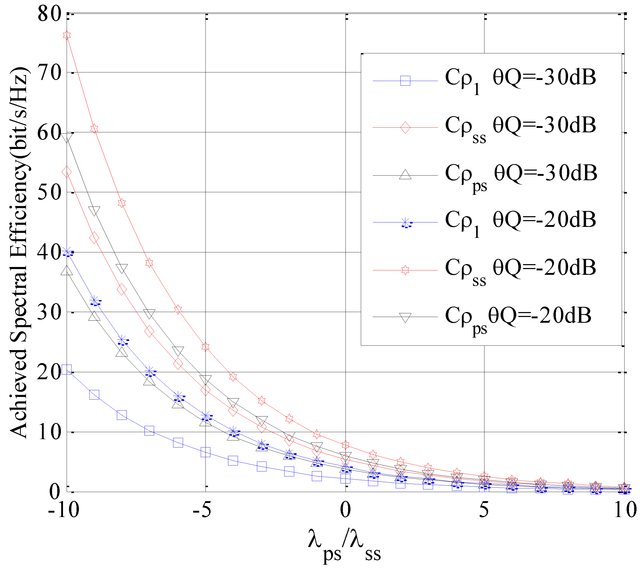
In the third simulation, both the influences of
gps and
gss are evaluated. Suppose
N = 40,
M = 1. The
is analyzed with
for different
θQ values. The simulation result is depicted in
Figure 8.
As depicted in
Figure 8, it is clearly observed that the
of the SUTCH decreases with the increase of
. Meantime, the
of the SUTCH decreases with the decrease of
θQ. This is due to the fact that with the increase of
, the attenuation of
gps is decreased while that of
gss is increased. Consequently, the
of SUTCH is lower with the same transmitting power. On the other hand, with the decrease of
θQ, the power allocated to each selected subchannel is bound to be reduced, which will lead to the deterioration in the
of the SUTCH.
Compared comprehensively, the of the SUTCH with ρ1 has the lowest value, since it just ignores any a priori knowledge of subchannel’s status. However, under different conditions, the performance of the ρss and ρps are different. When the ratio of M/N is small, the best subchannel selection policy is ρss. However, if the ratio of M/N is large, the best subchannel selection policy is ρps.
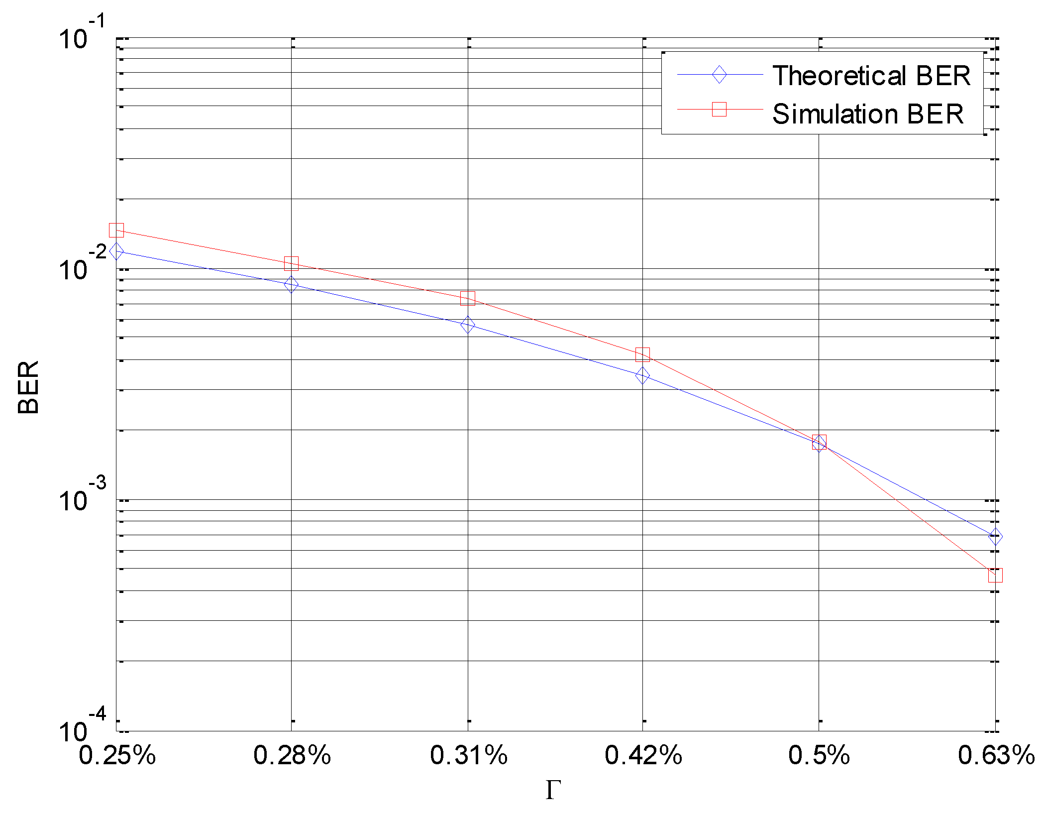
In the fourth simulation, as mentioned above, in Equation (49), the BER of SUCCH is derived. Therefore, Monte Carlo Simulation is used to prove its rationality. The simulation parameters are shown in
Table 1. Suppose
.
In
Figure 9, the Simulation BER is calculated by Monte Carlo Simulation Experiment, while the Theoretical BER is calculated by Equation (49). As depicted in
Figure 9, the simulation BER follows the Theoretical BER very closely.
As mentioned in
Section 4, the trade-off problem between the reliability of the SUCCH and the efficiency of the SUTCH is discussed. Here, suppose the arrival rate of the authorized PUs accessing to the subchannels follows a Poisson distribution. Simulation parameters are shown in
Table 2. Suppose
represents the arrival rate of the PUs in accessible subchannels.
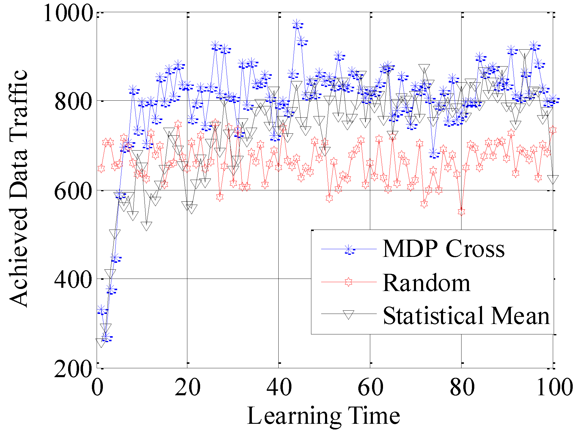
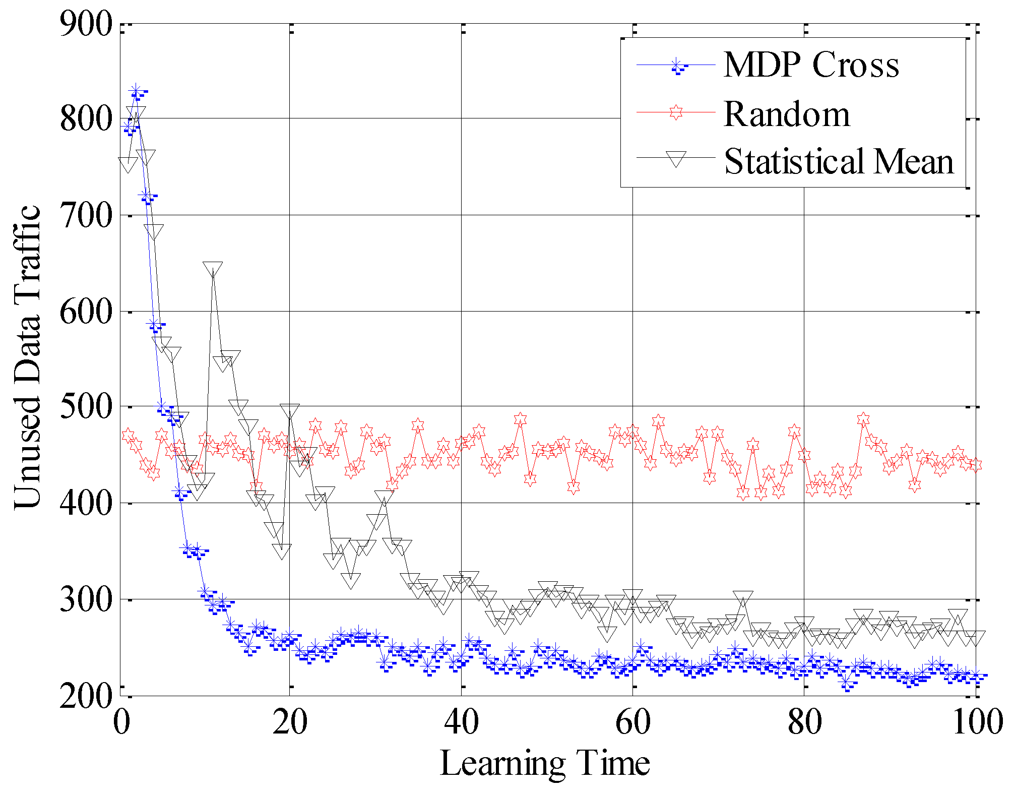
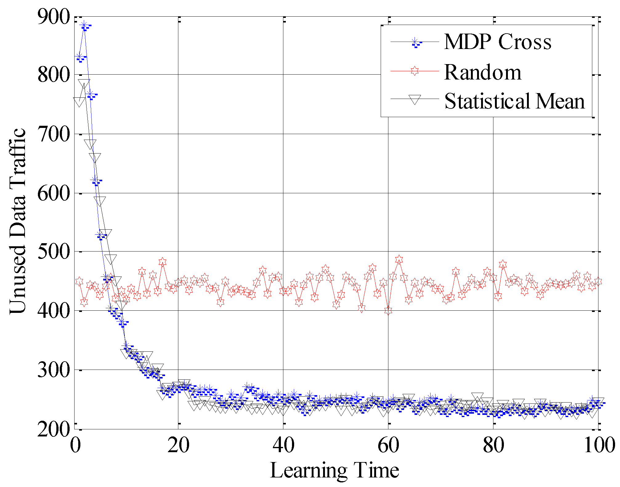
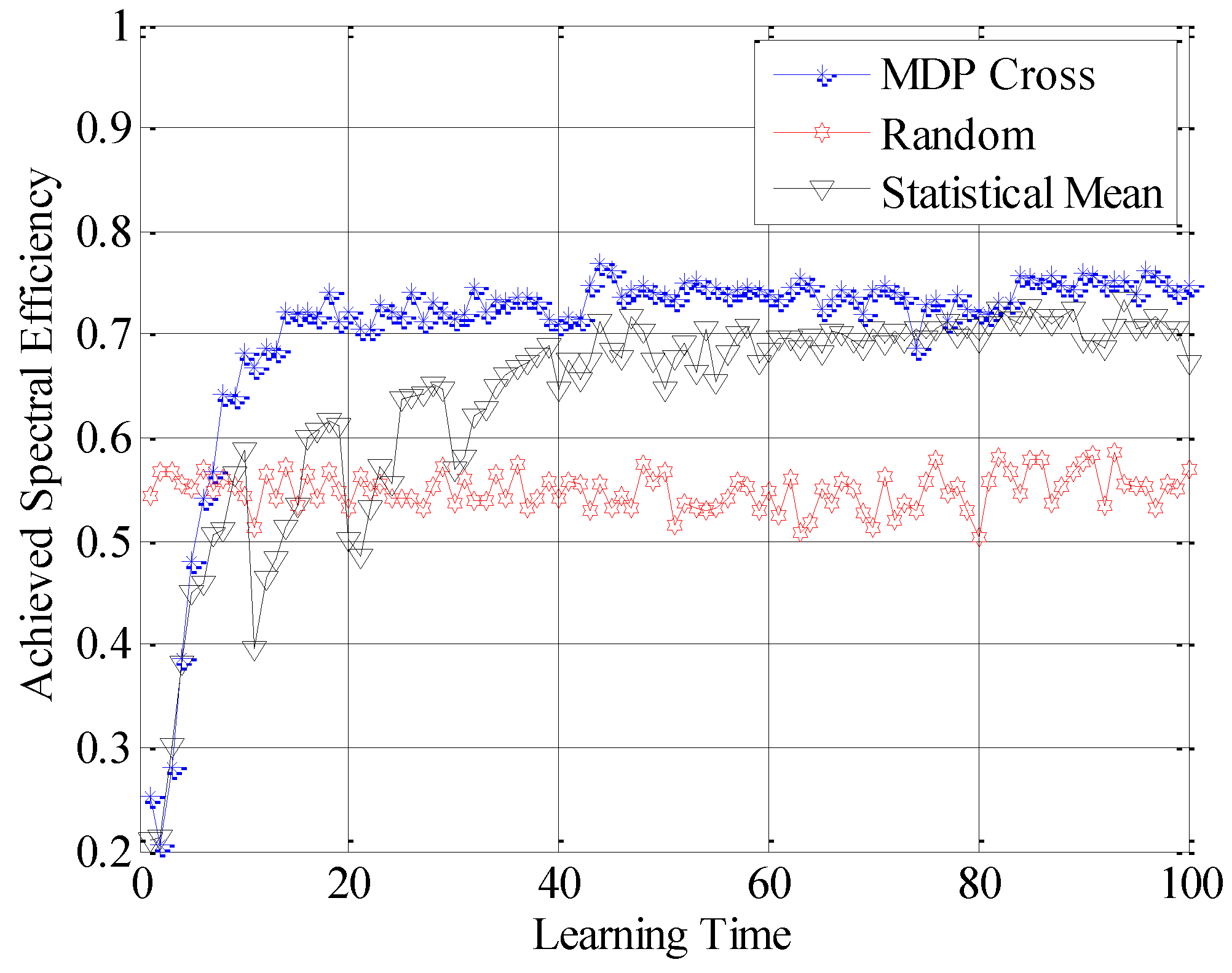
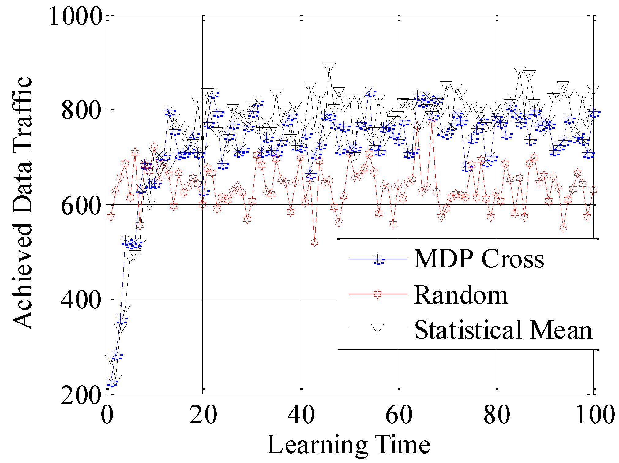
In the fifth simulation, the achieved spectral efficiency, achieved data traffic and unused data traffic are used to compare the accessible performance of the three different selection policies. Here, achieved spectral efficiency represents the proportion between data traffic and unused data traffic. Data traffic is the total amount of unit data traffic when the SUTCH has successfully accessed to the idle subchannel, while unused data traffic is the achievable amount of unit data traffic during the time cost in establishing the connection.
In
Figure 10,
Figure 11 and
Figure 12, the different performances of the three strategies are shown in detail. Random strategy has the worst accessible performance, because it simply chooses the loading factor Г randomly without proper accessible strategies. Meanwhile, the accessible performance of MDP Cross is better than that of Statistical Mean. Furthermore, the fluctuation of performance curve of MDP Cross is lower than that of Statistical Mean. It is due to the fact that, in the simulation, suppose
j = 1, 2, …, 6 ∈ [80, 160] the state parameters of the accessible subchannel are changing very fast, therefore, it is a quick-changing subchannel environment. In the quick-changing subchannel environment, the history state information of subchannel environment is changing very fast. However, Statistical Mean will use a lot of history information, so the fast-changing of history information will make a bad influence on choosing the optimal allocation strategy of Г. Therefore, the accessible strategy of MDP Cross fits better in the quick-changing subchannel environment.
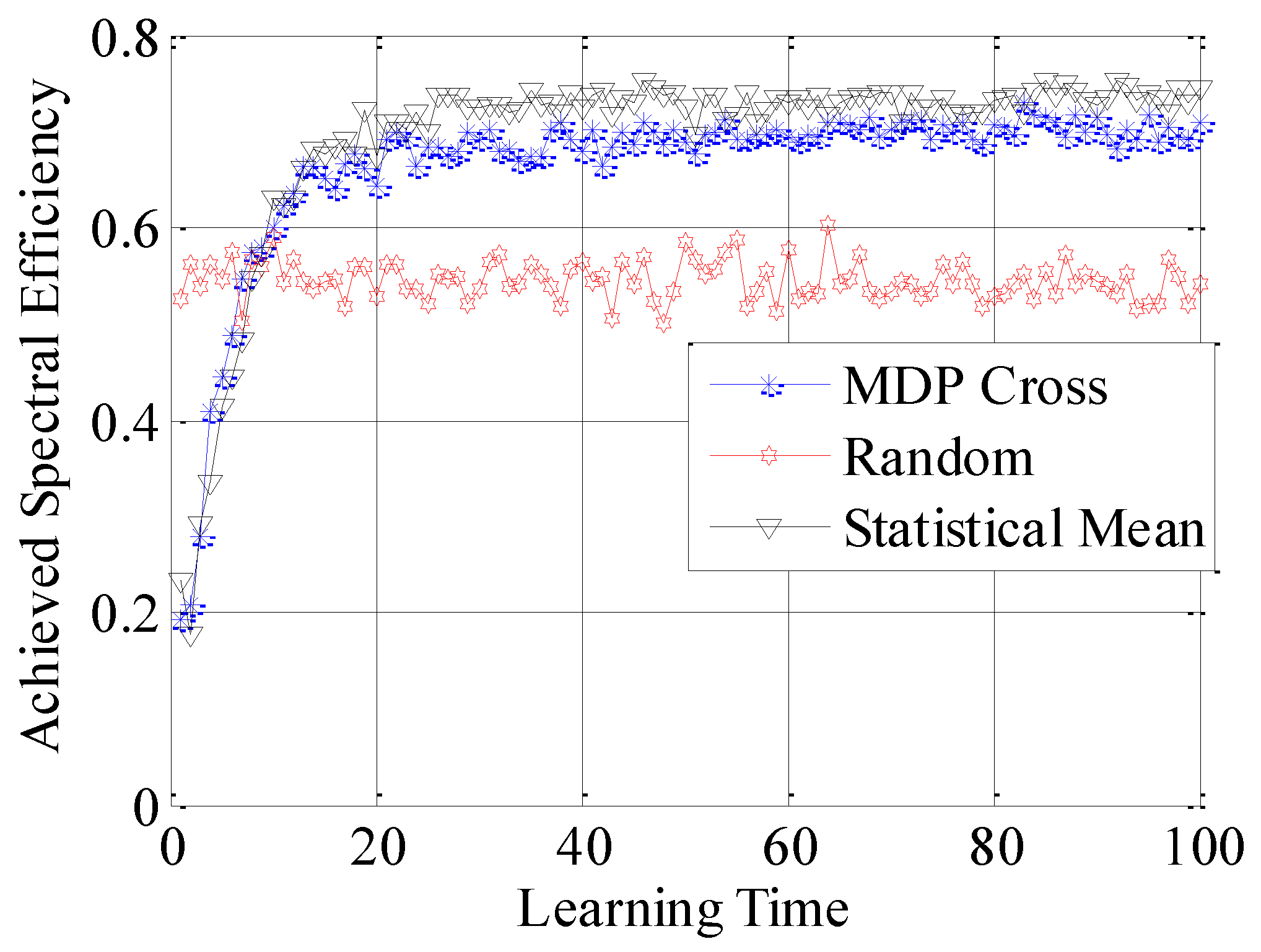
In the sixth simulation, different performances of the three strategies under constant application scenarios are shown in
Figure 13,
Figure 14 and
Figure 15. Suppose
is defined as constant, which is shown as follows:
As shown in these figures, the Random strategy still has the worst accessible performance. Meanwhile, the accessible performance of Statistical Mean is better than that of MDP Cross. Furthermore, the fluctuation of the performance curve of Statistical Mean is lower than that of MDP Cross. It is due to the fact that, in a slow-changing subchannel environment, the slow-changing of the history information will have a good influence on choosing the optimal allocation strategy of Г. Therefore, the accessible strategy of Statistical Mean fits better in the slow-changing subchannel environment.
In addition, as shown from
Figure 10 to
Figure 15, both Statistical Mean and MDP Cross can learn and adapt to the subchannel environment, and converge to a stable state in a short time. Meanwhile, they have the same rate of convergence. According to the analysis in
Section 4, both Statistical Mean and MDP Cross have low computation complexity. Therefore, they can be adopted in practice.


