Article

Intelligent Condition Diagnosis Method Based on Adaptive Statistic Test Filter and Diagnostic Bayesian Network

1
Jiangsu Key Laboratory of Advanced Food Manufacturing Equipment and Technology, Jiangnan University, 1800 Li Hu Avenue, Wuxi 214122, China
2
Graduate School of Bioresources, Mie University/1577 Kurimamachiya-cho, Tsu, Mie 514-8507, Japan
3
School of Mechanical & Electrical Engineering, Beijing University of Chemical Technology, Chao Yang District, Beijing 100029, China
*
Author to whom correspondence should be addressed.
Sensors 2016, 16(1), 76; https://doi.org/10.3390/s16010076
Submission received: 6 November 2015 / Revised: 18 December 2015 / Accepted: 30 December 2015 / Published: 8 January 2016
(This article belongs to the Section Physical Sensors)

Abstract

:
A new fault diagnosis method for rotating machinery based on adaptive statistic test filter (ASTF) and Diagnostic Bayesian Network (DBN) is presented in this paper. ASTF is proposed to obtain weak fault features under background noise, ASTF is based on statistic hypothesis testing in the frequency domain to evaluate similarity between reference signal (noise signal) and original signal, and remove the component of high similarity. The optimal level of significance α is obtained using particle swarm optimization (PSO). To evaluate the performance of the ASTF, evaluation factor Ipq is also defined. In addition, a simulation experiment is designed to verify the effectiveness and robustness of ASTF. A sensitive evaluation method using principal component analysis (PCA) is proposed to evaluate the sensitiveness of symptom parameters (SPs) for condition diagnosis. By this way, the good SPs that have high sensitiveness for condition diagnosis can be selected. A three-layer DBN is developed to identify condition of rotation machinery based on the Bayesian Belief Network (BBN) theory. Condition diagnosis experiment for rolling element bearings demonstrates the effectiveness of the proposed method.

1. Introduction

In the field of condition monitoring for rotating machinery, the vibration information, such as vibration accelerometer signal, vibration velocity signal, and vibration displacement signal, is often used for detecting faults and distinguishing fault types. Feature extraction of vibration signals is important for condition diagnosis [1,2]. However, feature extraction for condition diagnosis is difficult because the vibration signals measured for condition diagnosis contain strong noise component. Useful information is buried under stronger noise. In such case, the feature of machine condition could not be obtained and even the wrong conclusion will be induced. Thus, it is important that the feature of the signal can be sensitively extracted at the state change of a machine [3].
Many studies based on vibration signal processing technology have been carried out with the goal of machinery condition diagnosis [4,5,6,7]. Fourier analysis has been the dominating signal processing tool for condition diagnosis. In [8], Fourier analysis was used to identify the gear faults in planet cage. In [9], Fourier transform has been applied to detect rolling bearing faults. Unfortunately, there are some limitations of the Fourier transform, such as the fact that the signal to be analyzed must be strictly periodic or stationary. However, in practice, machinery operate under unsteady condition, such as varied rotating speed and operating load. In such case, even though the machinery is in the normal state, the spectrum feature and the frequency components of vibration signal are always changing with time. Thus the Fourier transform has no application to analyze non-stationary signal and can not reveal the inherent information of non-stationary signals [10,11]. Time frequency analysis methods, such as Wavelet Transforms (WT), Short Time Fourier Transform (STFT), etc., are effective tools for analyzing the non-stationary signals. These technologies can simultaneously provide the joint distribution information of signals in time domain and frequency domain, and describe the energy density or intensity of the signal at different times and frequencies. In [12], STFT and Hilbert-Huang transform (HHT) analysis were integrated to detect faults of ball bearings for wind turbine. However, the result of the STFT method depends on the choice of the windows size. Moreover, computational cost the STFT is high. WT has got huge success in fault diagnostics of rotating machinery for its ability to focus on localized structures in time frequency domain. WT can decompose the signal into many basis functions and extract signal features through change of the scales and time shifts of the basis function. In [13], WT method was employed to extract fault features of external load changing and the asymmetry of three-phase in induction motor. In [14], the broken-bar fault of induction motor was detected based on discrete WT. However, the feature extraction results of WT rest with the choice of wavelet basis function. Only selecting the appropriate basis function, the features of signal can work well to detect faults. In addition, due to the limited length of the wavelet base function, energy loss is inevitable [15]. Empirical mode decomposition (EMD) technique was proposed by Huang et al., for non-linear and non-stationary signal processing. EMD is a self adaptive signal processing technology that could decompose a non-linear and non-stationary signal into a set of intrinsic mode functions (IMFs). However, undesired frequency components in results and undesired low amplitude IMFs at the low-frequency region remain unsolved in EMD [16,17,18,19]. In addition, there are many noise cancelling methods that have also been applied, such as band pass filter [20], Kalman filter [21], Wiener filter [22], and so on. However, due to their flaws and shortcomings, these methods cannot always be applied to failure feature extraction. For example, band pass filter cannot cancel the wide band noise; when using Wiener filter and Kalman filter to process signal, the signal must follow the normal distribution.
The number of the artificial intelligence techniques, such as artificial neural networks (ANN), ant colony optimization (ACO), Bayesian belief network (BBN) etc., have been widely applied to fault diagnosis of plant machinery. In [23], three architecture NN, single-layer, multilayer perceptron network and counter propagation network, were introduced to detect 10 faults of a heat exchanger. In [2], an improved NN called partially-linearized neural network (PLNN) was presented to distinguishing the three types defect occurred in a rolling bearing. However, NN is not suitable for dealing with ambiguous diagnosis problems, and will never converge if SPs calculated by signals measured in different states have the same value. ACO algorithm imitates the behavior to solve optimization problems. In [24], ACO and DWT were integrated to detect faults of a rolling bearing used in the centrifugal fan system. However, ACO method is easy to trap into local optimum. In many cases, the optimization solution cannot be found. BBN is a powerful tool to represent and reason about complex systems with uncertain, incomplete and conflicting information [25,26]. A BBN enables us to model and reason about uncertainty, ideally suited for diagnosing real world problems where uncertain incomplete data exist. Therefore, it is a suitable solution for troubleshooting complex rotation machinery systems. In the last decades, BBN has been widely applied in condition diagnosis of plant machinery. References [27,28,29] are successful cases of BBN being used to detect fault of complex systems, such as nuclear power systems [27], aircraft engines [28], semiconductor manufacturing systems [29], etc.
To extract the fault feature of signals more effectively and discriminate conditions of rotation machinery more correctly, a novel method based on adaptive statistic test filter and Diagnostic Bayesian Network algorithm (DBN) for condition diagnosis of rotating machinery is presented. Structure of this paper is as follows: Section 2 instructs feature extraction method based on ASTF and evaluation factor Ipq. The optimal level of significance α is obtained by using PSO. In Section 3, the ten SPs for condition diagnosis are defined and PCA is employed to obtain high sensitive SPs for condition diagnosis. In 
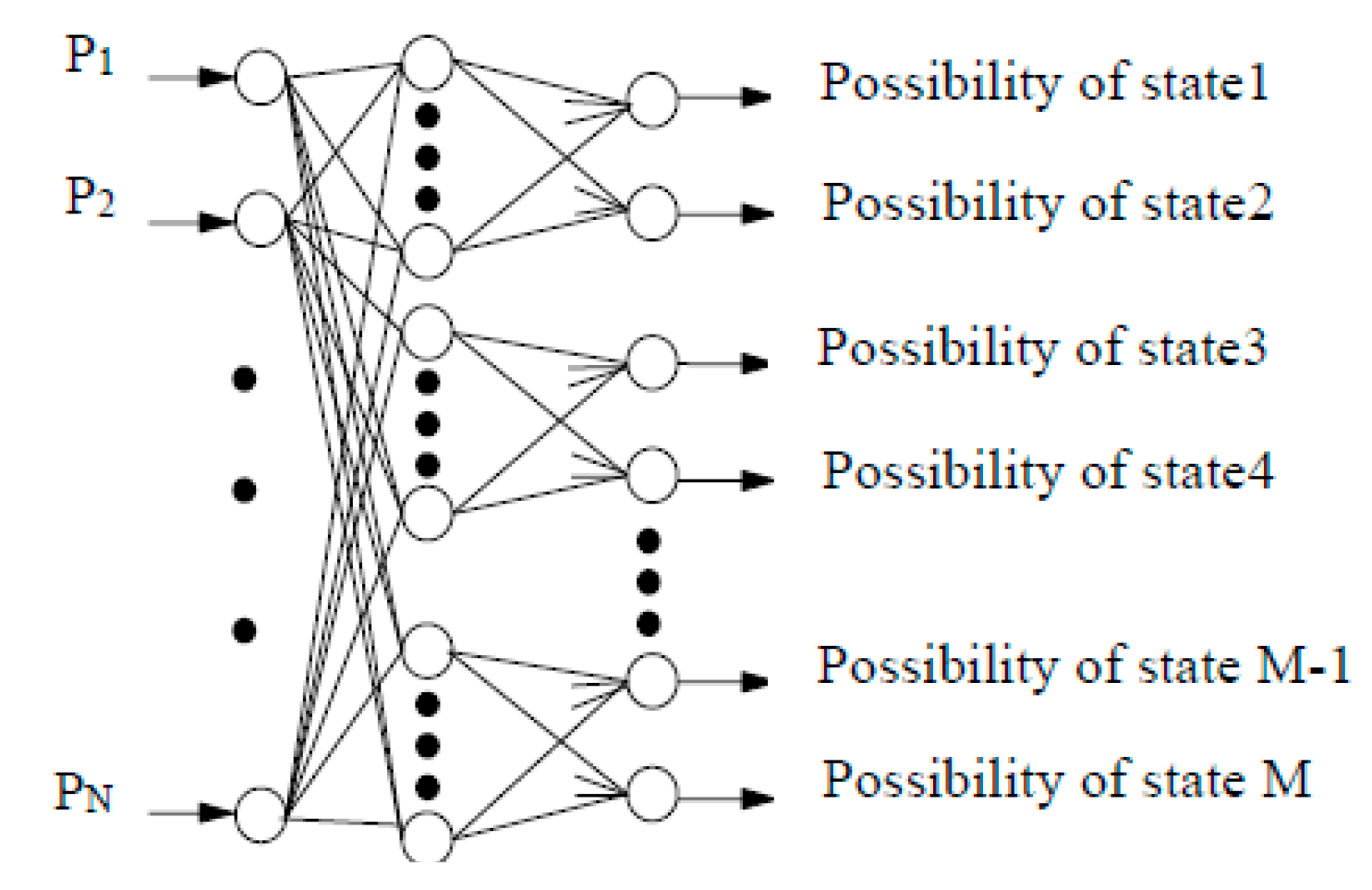
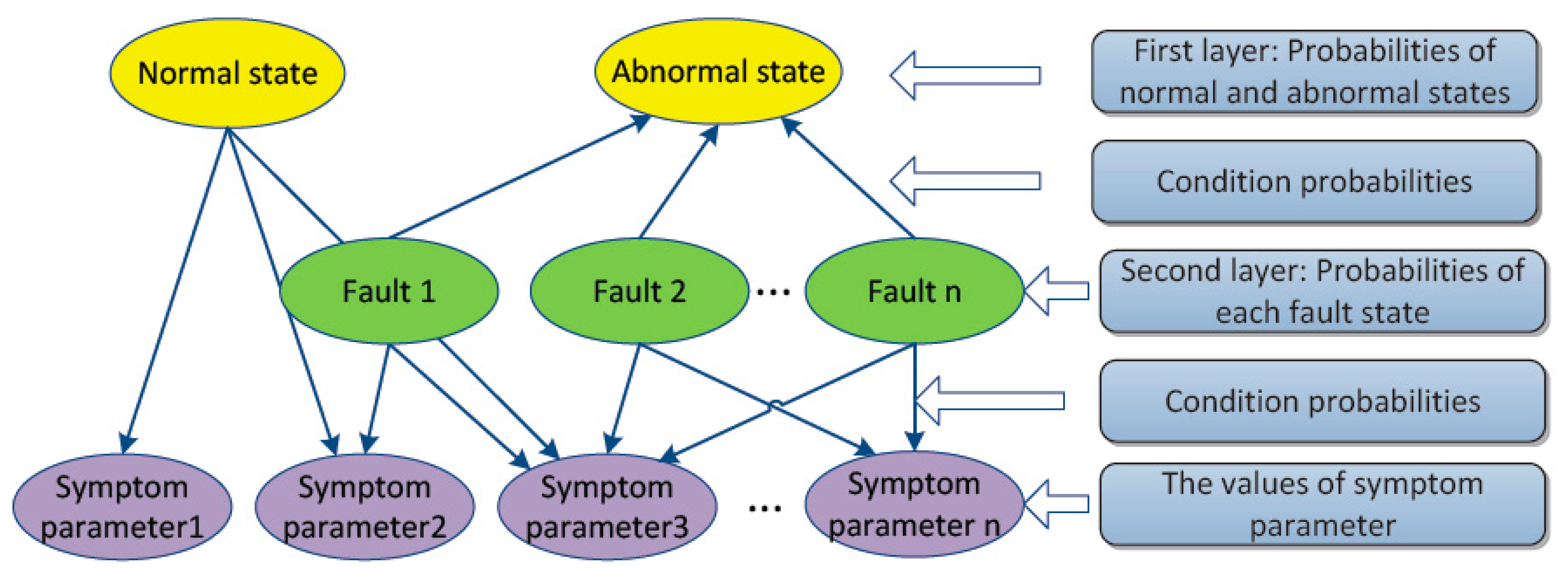
Section 4, a three-layer DBN is built to identify condition of rotation machinery based on BBN theory. Section 5 shows a practical example of fault diagnosis for verifying the effectiveness of the proposed method. Summary and conclusions are given in Section 6.

2. Feature Extraction by ASTF

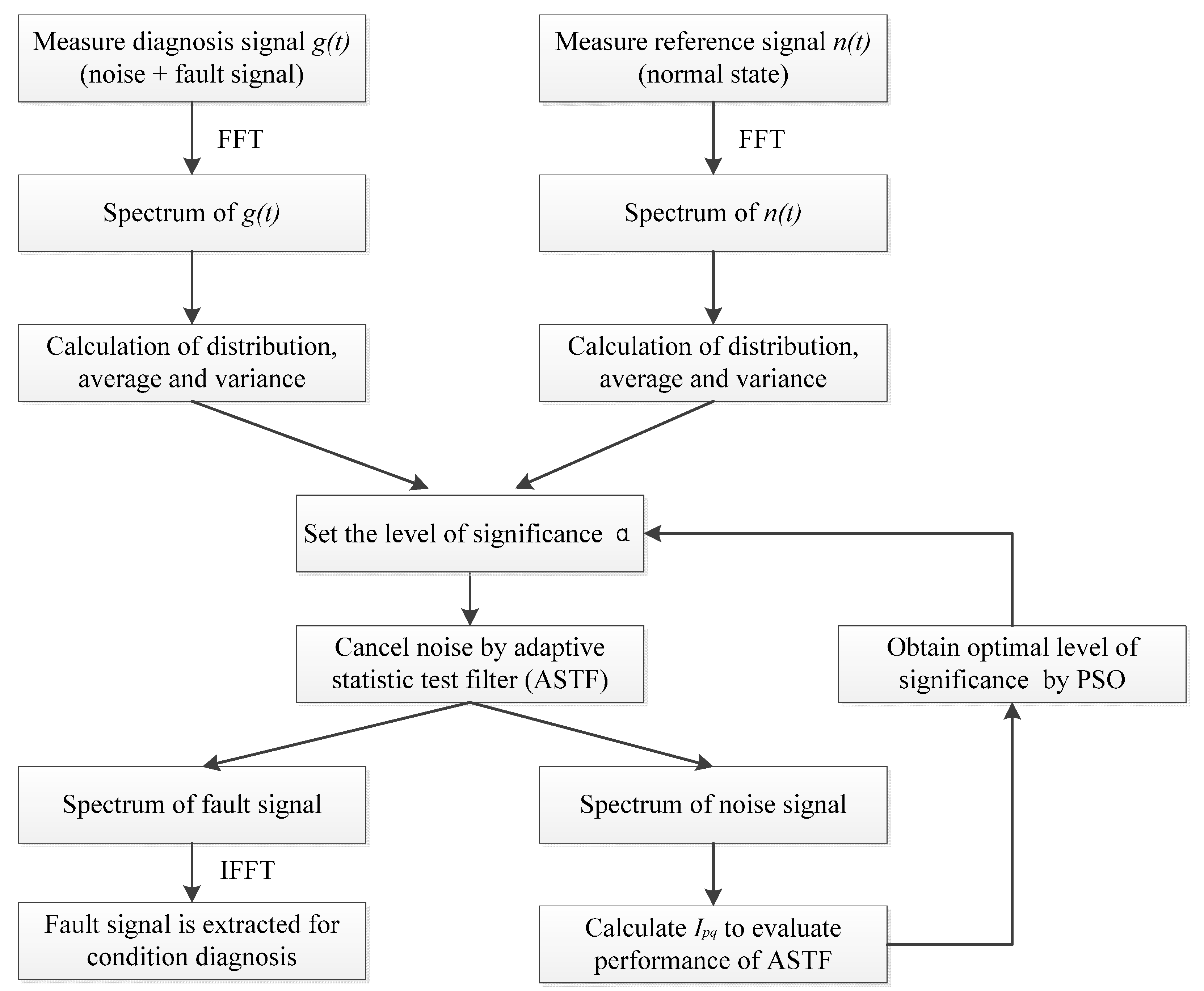
In this study, a new weak fault feature extraction method called adaptive statistic test filter (ASTF) is proposed. Principle of ASTF is based on statistic hypothesis testing in the frequency domain to evaluate similarity between reference signal (noise signal) and original signal, and remove the component of high similarity. Otherwise, the optimal level of significance α is obtained using PSO. The procedure for applying STF for the condition diagnosis is proposed, as shown in Figure 1.
Figure 1. Procedure for applying the ASTF for the condition diagnosis.
Sensors 16 00076 g001
The reference signal n(t) is measured in a normal state in advance. The original signal g(t) is measured in the state to be detected and polluted by noise. μ n ( f ) and μ g ( f ) indicate the average value of n(t) and g(t) in the frequency domain, respectively; and σ n 2 ( f ) and σ g 2 ( f ) indicate the variance value of n(t) and g(t) in the frequency domain, respectively. The two null hypotheses are as follows:
H 1 σ 2 g ( f ) = σ 2 n ( f )
H 0 μ g ( f ) = μ n ( f )
Firstly, σ 2 g ( f ) = σ 2 n ( f ) is verified by F test with m − 1 degree of freedom, and F = Sn2/Sg2.
S g 2 ( f ) = j = 1 m g ( f ) 2 / ( m 1 ) g ¯ ( f ) 2
S n 2 ( f ) = j = 1 m n ( f ) 2 / ( m 1 ) n ¯ ( f ) 2
If σ 2 g ( f ) = σ 2 n ( f ) , μ g ( f ) = μ n ( f ) is verified by t test with 2m − 2 degree of freedom, and t = { g ¯ ( f ) n ¯ ( f ) } / S 2 / m .
here,
S 2 = { ( m 1 ) S g 2 + ( m 1 ) S n 2 } / ( 2 m 2 )
If σ 2 g ( f ) σ 2 n ( f ) , t = { g ¯ ( f ) n ¯ ( f ) } / S g 2 ( f ) / m + S n 2 ( f ) / m .
m = ( S g 2 / m + S n 2 / m ) 2 /    [ { S g 4 / m 2 ( m 1 ) } + { S n 4 / m 2 ( m 1 ) } ]
If both null hypotheses would prove to be received, the spectrum component of the original signal g(t) at the frequency f is similar to that of the reference signal n(t). The component at the frequency f does not contain fault information and will be removed. If alternative hypothesis is denied, it means that the spectrum component of the original signal g(t) at the frequency f is not similar to that of the reference signal n(t). The component at the frequency f contains fault information.
After STF, the original signal g(t) is decomposed into estimated fault signal g*(t) and estimated noise signal n*(t). In order to appraise the performance of STF, evaluation factor Ipq is defined. qi and qi* are the number that n(t) and n*(t) cross over some level i of the vertical coordinate of the power spectrum Fn2(fk) with a positive slope in unit time and can be calculated as follows:
q i = σ v 2 π σ x e n i 2 / 2 σ x 2
p i = 2 π σ v q i
σ x 2 = 0 F n 2 ( f k ) d f k
σ v 2 = 0 ( 2 π f k ) 2 F n 2 ( f k ) d f k
where i = 1 ~ K ,    n i = min { n ( t ) } ~ max { n ( t ) } .
Ipq is defined as follows:
I p q = i = 1 K | log ( q i q i * ) | / K + i = 1 K | log ( p i p i * ) | / K
It is obvious that the smaller the value of the Ipq, the more similar n(t) and n*(t) will be, and therefore, the better the STF will be. Thus, Ipq is able to express the similarity degree between n(t) and n*(t); that is to say, Ipq can be used to evaluate the performance of STF.
To obtain optimal level of significance α, an adaptive PSO algorithm is proposed in this paper. PSO algorithm is based on groups, and solves an unconstrained D-dimensional optimization problem by minimization of the objective or the fitness function [30,31,32]. In this study, the fitness function is the evaluation factor Ipq (Equation (11)). In PSO algorithm, each particle keeps track of its own position denoted by P ( i ) . l o c a t i o n = [ X i 1 , X i 2 X i D ] and velocity denoted by P ( i ) . v e l o c i t y = [ V i 1 , V i 2 V i R ] in the problem space, according to its own and neighboring particle experience [22,23,24]. The best previous position of particle is marked by the lowest fitness value and indicated by P ( i ) . b e s t = [ P i 1 , P i 2 P i R ] . The best position among all particles experienced discovered by the swarm, so far, is defined as g ( i ) . b e s t = [ g i 1 , g i 2 g i R ] . Then, the new positions and velocities of the particles are updated by the following equations:
P ( i ) . v e l o c i t y ( t + 1 ) = ω   P ( i ) . v e l o c i t y ( t ) + η 1 r 1 [ P ( i ) . b e s t ( t ) P ( i ) . l o c a t i o n ( t ) ] + η 2 r 2 [ g ( i ) b e s t ( t ) P ( i ) . l o c a t i o n ( t ) ]
P ( i ) . l o c a t i o n ( t + 1 ) = P ( i ) . l o c a t i o n ( t ) + P ( i ) . v e l o c i t y ( t + 1 )
where r1 and r2 indicate random numbers between 0~1. η1 is the cognitive parameter (acceleration coefficient). η2 is the social parameter (acceleration coefficient). The inertia weight ω controls the previous velocity of particle, and ω adaptively adjust as follows:
ω = { k 1 + 0.5 q R > 0.05 k 2 + 0.5 q R 0.05
where q is a random number with a uniform probability between 0~1; k1 and k2 are parameters, and k1 > k2 , the choice of k1 and k2 is determined experimentally, here k1 = 0.5 and k2 = 0.2. R indicates change rate, which defined as Equation (15); if R is greater than 0.05, PSO is in the exploration stage, a large ω is beneficial to the algorithm’s convergence; if R is less than 0.05, PSO is in the development stage, a small ω is beneficial to searching optimum point.
R = | I p q ( t + 5 ) I p q ( t ) | | I p q ( t ) |
where Ipq(t) is minimization evaluation factor value of the t-th iteration. Ipq(t + 5) is minimization evaluation factor value of the (t + 5)-th iteration.
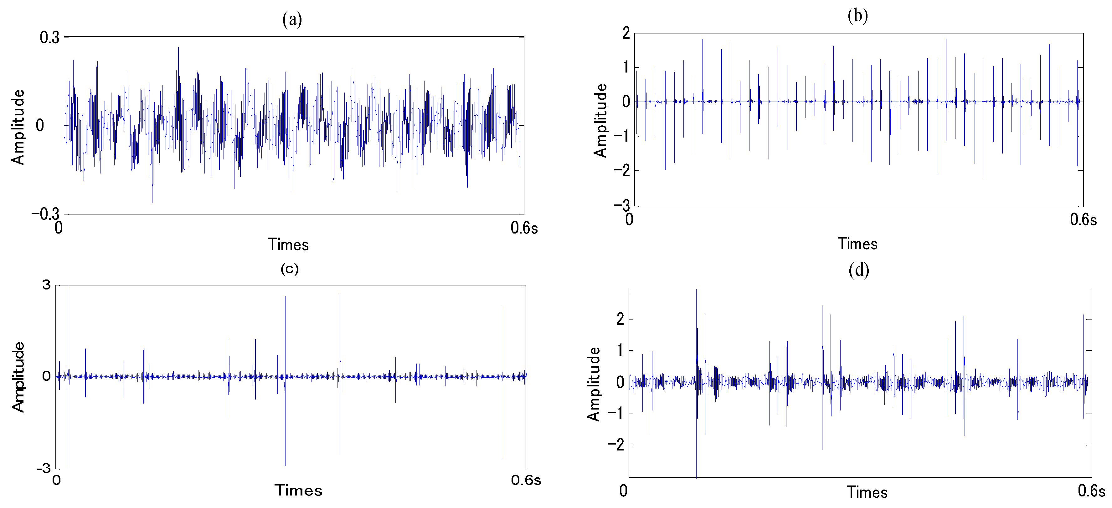
In order to test and verify capability of ASTF, a simulation experiment is designed. Ten set signals that consist of the impulsive signal with the period of 0.015 s and random white Gaussian noise are produced using Matlab software to simulate a bearing fault. These noisy signals are processed by ASTF and a high pass filter with 5000 Hz cut off frequency, respectively. The performances of denoising are estimated based on SNR. Mathematical expression of the impulsive signal is shown in Equation (16).
x ( t ) = x 0 e ξ ω n t sin ω n 1 ξ 2 t
where ξ indicates coefficient of damping and ξ = 0.2; ωn expresses natural frequency and ωn = 3 kHz; and x0 denotes displacement constant and x0 = 2.
Figure 2 shows the SNR of denoised signals processed by ASTF and high pass filter. As shown in Figure 2, all of the SNR values of denoised signals after ASTF are much greater than high pass filter. Then, ASTF method is effective and has high robustness for signal denoising.
Figure 2. Signal-to-Noise Ratio (SNR) of denoised signals processed by each method.
Sensors 16 00076 g002

3. Symptom Parameters for Fault Diagnosis and Sensitivity Evaluation

3.1. Symptom Parameters for Fault Diagnosis

The number of SPs reflect plant machinery condition have been defined in the pattern recognition field [33]. In this study, ten SPs in the time domain are considered.
P 1 = σ x ¯
P 2 = i = 1 N x i 2 σ 2
P 3 = | i = 1 N ( x i x ¯ ) 3 | N σ 3
P 4 = i = 1 N ( x i x ¯ ) 4 N σ 4
where, xi is digital data of vibration signal. x ¯ is the mean value of xi, x ¯ = i = 1 N x i N . σ is standard deviation of xi, σ = i = 1 N ( x i x ¯ ) 2 N 1 .
P 5 = x p ¯ x ¯
P 6 = x p ¯ σ
P 7 = | i = 1 N p ( x p i x p ¯ ) 3 | N p σ p 3
P 8 = | i = 1 N p ( x p i x p ¯ ) 4 | N p σ p 4
where, xpi is the peak value of xi. x ¯ p and σ p are the mean value and standard deviation of xpi, respectively.
P 9 = | i = 1 N v ( x v i x v ¯ ) 3 | N v σ v 3
P 10 = | i = 1 N v ( x v i x v ¯ ) 4 | N v σ v 4
where, xvi is the valley value of xi. x ¯ v and σ v are the mean value and standard deviation of xvi, respectively.

3.2. High Sensitivity Symptom Parameters Obtained by PCA

PCA is a statistical analytical tool used to explore, sort and group data. PCA takes a large number of correlated variables and transform these data into a smaller number of uncorrelated variables known as principal components. The first few principal components contain most of the information and the discriminatory features [34].
Define a data matrix with size m × n, where m is the number of identifying states and n is the number of SPs, whose covariance matrix has eigenvalue λi and eigenvector ai (a is loading of the principal component and can express the importance of the SPs for each principal component) and I = 1 − n with λ1 ≥ λ2 ≥…≥ λn. Principal components Zi and the cumulative contribution rate of the principal components ηi can be calculated as follows:
{ Z 1 Z n } = [ a 11 a 1 n a m 1 a m n ] = A P
η i = j = 1 i λ j / k = 1 n λ k
where Pi indicates a symptom parameter, I = 1 − n.

4. Bayesian Belief Network

BBN is a probability network based on graphical network model for describing causal uncertainties between variables. It is built for uncertainty modeling and reasoning, and has a great advantage in diagnosing fault caused by uncertainty and correlation of the complex systems.

4.1. Bayesian Inference

Supposing A is a random event and B is the event that is root causes generating A, conditional probabilities P(A|B) between A and B can be calculated as follows:
P ( A | B ) = P ( A B ) P ( B ) = P ( A ) P ( B | A ) P ( B )
where P(AB) is the joint probability, P(AB) = P(B)∙P(A|B)=P(A)∙P(B|A).
Supposing Bi (i = 1, 2, ..., n) are mutually exclusive and complete set of root causes generating A, the marginal probability of A is
P ( A ) = i = 1 n P ( B i ) P ( A | B i )
The conditional and marginal probabilities of A and Bi is
P ( B i | A ) = P ( A B i ) P ( A ) = P ( B i ) P ( A | B i ) i = 1 n P ( B i ) P ( A | B i )
In Equation (31), P(Bi) and P(A/Bi) express prior probabilities and prior conditional probabilities, respectively. P(Bi/A) indicates posterior probability. When using the Bayesian inference for fault diagnosis, Bi represents an equipment condition and A represents a SP. The prior probability of the SPBi(P(Bi)) and the conditional probability of equipment condition A given BiP(A/Bi) can be obtained from expert experience or statistical data. Then, the posterior probability P(Bi/A) can be obtained by Equation (31). If this posterior probability is high, the condition Bi can be confirmed at the given A, and the equipment condition is judged Bi.

4.2. Topology of Bayesian Belief Network

A BBN consists of a number of nodes, directed links, and probability tables. For a diagnostic BBN model, nodes represent variables that can be SP, equipment condition or observations. Directed links indicate casual relationships between the variables. In this paper, the purpose of building a diagnostic BBN is to reason the most likely mechanical condition based on the values of SP, given one or more SP values to calculate posterior probabilities of the cause. The calculus of posterior probability involves calculating the joint probability for the model (probabilities of all combined states for all nodes within the model). The network contains five nodes, X1, X2, X3, X4, and X5, with a structure of three layers (see in Figure 3). In terms of the definition of the three types of conditional independence, X1 is independent of X2; X1 is parent of X3 and X4. Given X1, X3 and X4 are conditionally independent of each other, X5 is independent of X1, X2, and X3. The following derivation indicates how to calculate the posterior conditional probability P(X4 = true|X5 = true).
P ( X 4 = true | X 5 = true ) = P ( X 4 = true | X 5 = true ) P ( X 5 = true ) = x 1 x 2 x 3 P ( X 1 X 2 X 3 X 4 = true , X 5 = true ) x 1 x 2 x 3 x 4 P ( X 1 X 2 X 3 X 4 , X 5 = true )
where P(X1, X2, X3,X4 = true|X5 = true) and P(X1, X2, X3,X4 ,X5 = true) involve calculating the joint probability of the model. The joint probability of this model P(X1, X2, X3, X4, X5) can be calculated as follows:
P ( X 1 X 2 X 3 X 4 , X 5 ) = i = 1 5 P ( X i | X 1 , , X i 1 ) = P ( X 1 ) P ( X 2 | X 1 ) P ( X 3 | X 1 X 2 ) P ( X 4 | X 1 X 2 X 3 ) P ( X 5 | X 1 X 2 X 3 X 4 )
Applying the independence assumption, the joint probability distribution can be simplified as follows:
P ( X 1 X 2 X 3 X 4 , X 5 ) = i = 1 5 P ( X i | P a i ) = P ( X 1 ) P ( X 2 ) P ( X 3 | X 1 ) P ( X 4 | X 1 X 2 ) P ( X 5 | X 4 )
Figure 3. General model of Bayesian Belief Network.
Sensors 16 00076 g003

4.3. Framework of Diagnostic Bayesian Network

In this study, Diagnostic Bayesian Network (DBN) is constructed for intelligent condition diagnosis. As shown in Figure 4, the proposed DBN consists of three layers. The first layer is normal and abnormal states. The second layer is fault states, and the last layer is SPs calculated from the signals processed by ASTF.
In the proposed DBN, prior probabilities of root nodes are needed and conditional probabilities are also needed to represent direct probabilistic dependences among nodes in the three layers. Here, all machine states are regarded as parent nodes, and the prior probabilities of state i (Si) can be obtained as follows:
P ( S i ) = N S i N
where NSi represents the sample size of state i, and N indicates the total number of samples.
The conditional probabilities of each node are obtained as follows
P ( S P = x i | S i ) = N S i x i N S i N S i x i 0 P ( S P = x i | S i ) = 1 N N S i + N x i N i f N S i x i = 0
where SP represents the values of symptom parameters, and N S i x i indicates the sample size of state i, when SP = xi.
Figure 4. Structure of Diagnostic Bayesian Network.
Sensors 16 00076 g004

5. Diagnosis and Application

5.1. Condition Diagnosis by Proposed Method

In this section, an experimental setup is designed to evaluate the effectiveness of the method proposed in this paper. The flowchart of the condition diagnostic procedure is shown in Figure 5.
Figure 6 shows the experimental bench for condition diagnosis test, which includes a servo motor, rotor system and loading equipment. The NSK 205 ball bearing is used for bearing condition diagnosis. As shown in Figure 7, three types fault: the outer defect, the inner defect, and the roller element defect were artificially made by using electro discharge machining with fault width was 0.3 mm, and fault depth was 0.025 mm.
In the present work, the original vibration signals in each state were measured by the accelerometer (PCB MA352A60, PCB Piezotronics Inc., New York, NY, USA) with 50,000 Hz sampling frequency. The accelerometer was fixed on vertical direction of the bearing. While the vibration signals were being obtained, the speed of servo motor was 800 rpm, and a 150 kg load was also transported on the rotating shaft by the loading equipment (RCS2-RA13R, IAI Co. Ltd., Shizuoka, Japan). All the data were recorded and transformed by a collection system includes a sensor signal conditioner (PCB ICP Model 480C02, PCB Piezotronics Inc., New York, NY, USA) and a signal recorder (Scope Coder DL750, YOKOGAWA Co. Ltd. Tokyo, Japan). Obtained data was divided to two sets, one set includes 80 samples and was used to train diagnosis system; the other set includes 20 samples and was used for condition identification test. Figure 8 shows the original vibration signal in each state, and Figure 9 shows the vibration signal after ASTF.
Figure 5. Flowchart for the condition diagnostic procedure.
Sensors 16 00076 g005
Figure 6. Experimental system for bearing fault diagnosis.
Sensors 16 00076 g006
Figure 7. Bearing defects: (a) outer-race defect; (b) inner-race defect; and (c) roller defect.
Sensors 16 00076 g007
Figure 8. Original vibration signal: (a) normal state; (b) outer-race defect; (c) inner-race defect; and (d) roller defect.
Sensors 16 00076 g008
Figure 9. Vibration signal after ASTF: (a) normal state; (b) outer-race defect; (c) inner-race defect; and (d) roller defect.
Sensors 16 00076 g009
In this study, the SPs that contain the most information and have high sensitivity for each state are selected by PCA. As an example, parts of the selection results are shown in Table 1 and Table 2; P1, P2, P6, P8 and P9 have high sensitivity for distinguishing normal state and abnormal state. Because the weight coefficients for P1, P2, P6, P8 and P9, the first principal component, are larger than those of the other, the contribution rate of the first principal component is larger than 0.86, which contains enough information and discriminatory features to identify the normal state and abnormal state. Similarly, the SPs for other states can also be selected.
In this paper, the DBN for distinguishing conditions of a rolling bearing was built as shown in Figure 10. The proposed DBN consists of three layers. The first layer is normal and abnormal states. The second layer is main failures such as outer-race defect, inner-race defect, and roller element defect, which often occurred in a rolling bearing. The last layer is SPs shown in Table 2. The prior probabilities and the conditional probabilities were obtained by Equations (35) and (36). All of the SPs were divided into five levels, 1, 2, 3, 4 and 5, which indicate very small, small, middle, big and very big levels, respectively. As an example, parts of the training sample data are shown in Table 3.
Figure 10. DBN for distinguishing conditions of a rolling bearing.
Sensors 16 00076 g010
Table 1. First principal component of SPs.
Weight Coefficients for Each Symptom ParameterContribution Rate
P1P2P3P4P5P6P7P8P9P10η1
N:O0.990.91−0.62−0.75−0.330.85−0.690.880.790.210.88
N:I0.930.87−0.53−0.32−0.650.780.110.920.81−0.420.86
N:R0.991.0−0.9−0.36−0.750.9−0.220.860.91−0.360.89
O:I0.871.0−0.560.990.88−0.66−0.710.98-0.560.380.90
O:R0.990.99−0.370.930.95−0.58−0.620.98-0.790.860.85
I:R0.970.86−0.780.360.91−0.55−0.110.87-0.910.950.86
Table 2. Selection result of the SPs for distinguishing each state.
StateSelection result
NormalP1, P2, P6, P8, P9
Outer-race defectP1, P2, P4,P5, P8,
Inner-race defectP1, P2, P5, P8,
Roller-element defectP1, P2, P5, P8, P10,
Table 3. Training sample data.
StateNon-dimensional Symptom Parameters
P1P2P3P4P5P6P7P8P9P10
Normal1111111111
1111121112
1111121211
1111111112
..............................
Outer-race defect2314431323
3314431324
2213431325
3314431323
..............................
Inner-race defect3121121344
4122155454
3112243444
3111133332
..............................
Roller element defect5513553445
4424553555
4453553435
4423553445
..............................
To verify the diagnostic capability of the diagnosis methods proposed in this paper, we used the data measured in each state had not been used to train the DBN system. They can correctly and quickly diagnose those faults with the possibility grades of the corresponding states. In the test of normal state, the successful diagnosis ratio is 100%. In the test of each faults, the successful diagnosis ratio of outer-race defect, inner-race defect and roller element defect states are 100%, 94% and 86%, respectively. Some diagnosis results are shown in Table 4, Table 5, Table 6 and Table 7.
Table 4. Diagnosis results of normal state.
Non-Dimensional Symptom ParametersStateJudge
P1P2P6P8P9NormalAbnormal
111110.960.04Normal
111210.890.11Normal
112110.910.09Normal
........................
Table 5. Diagnosis results of outer-race defect state.
Non-Dimensional Symptom ParametersStateJudge
P1P2P4P5P8Outer-Race DefectOther Faults
334430.990.01Outer-race defect
224430.890.11Outer-race defect
235430.860.14Outer-race defect
........................
Table 6. Diagnosis results of inner-race defect state.
Non-dimensional Symptom ParametersStateJudge
P1P2P5P8Inner-Race DefectOther Faults
41230.850.15Inner-race defect
32140.790.21Inner-race defect
31240.880.12Inner-race defect
.....................
Table 7. Diagnosis results of roller element defect state.
Non-dimensional Symptom ParametersStateJudge
P1P2P5P8P10Roller-Element DefectOther Faults
445550.750.25Roller-element defect
334550.680.32Roller-element defect
345450.660.34Roller-element defect
........................

5.2. Condition Diagnosis by NN

In this study, a back propagation NN shown in Figure 11 is also constructed for condition diagnosis of the roller bearing. The NN consists of three layers, the SPs calculated by vibration signals are entered into input layer, hidden layer includes 80 units, output layer is the possibility grades of each condition of roller bearing. Table 8 shows the parts of diagnosis results of NN. N, O, I and R indicate the normal, outer race defect, inner race defect and roller element defect states, respectively. The symbol × expresses the case that NN is incapable of identifying the fault type. As shown in Table 8, the normal and outer race defect states of roller bearing were correctly identified by NN. However, NN is incapable of identifying inner race defect and roller element defect states of roller bearing. The main reasons are that the vibration signals measured for condition diagnosis contain strong noise, there exist ambiguous relationships between the SPs and the fault types, and NN cannot deal with incomplete and conflicting information.
Figure 11. The back propagation NN for condition diagnosis.
Sensors 16 00076 g011
Table 8. Diagnosis results of NN.
P1P2P3P4P5P6P7P8P9P10NOIRJudge
0.020.060.136.132.241.01.984.722.0111.90.8680.0010.1350.012N
0.020.070.115.872.581.031.755.731.1510.10.8950.0010.0980.169N
0.030.160.151034.852.012.3366.33.051050.0630.8050.1770.055O
0.030.170.191064.622.152.6872.53.6699.70.0870.7960.2060.036O
0.020.110.2533.42.913.0610.880.78.491090.0560.0710.5320.405×
0.040.090.3248.93.651.959.6785.68.9894.90.0950.0410.5010.386×
0.050.320.4793.95.293.578.8711510.81240.0110.0950.4060.513×
0.060.260.681065.473.269.1312310.21390.0320.0860.3660.572×
.............................................

6. Conclusions

In order to detect the condition of rotating machinery at an early stage, a novel fault diagnosis method based on ASTF and DBN was presented. The main conclusions of this paper are summarized as follows:
  • The method of ASTF for extracting weak fault features under background noise was presented. The optimal level of significance α was obtained using PSO. To evaluate the performance of ASTF, evaluation factor Ipq was also defined. In addition, a simulation experiment was designed to verify the effectiveness and robustness of ASTF.
  • PCA based on statistical analysis theory was also presented to evaluate the sensitivities of SPs calculated via vibration signals measured in each state for condition identification.
  • A three-layer DBN was developed to identify condition of rotation machinery based on the BBN theory. It is effective and efficient in condition diagnosis based on uncertain, incomplete and conflicting information.
  • Study examples of diagnosis for a bearing were shown to demonstrate the effectiveness of the methods proposed in this paper. The verification results show that the bearing faults that often occur in roller bearings, such as the Outer race, the Inner race and the roller element defects, have been effectively identified by the proposed method in this paper. However, these bearing faults are difficult to detect using NN technology, because the vibration signals measured for condition diagnosis contain strong noise, there exist ambiguous relationships between the SPs and the fault types, and NN cannot deal with incomplete and conflicting information.
In summary, this paper verifies the capability of condition diagnosis method based on ASTF and DBN. In addition, soft sensor technique establish inference model of symptom parameters based on state-space model, and solves inference model of symptom parameters by parameter estimation method, such as Kalman filter and Bayesian filter. The condition diagnosis system includes two parts: feature extraction and condition identification. Soft sensor technique can be used of feature extraction and fusion, and condition identification can adopt artificial intelligence techniques, such as DBN, NN, etc. In the future, we will consider using soft sensor technique to extract features of signals.

Acknowledgments

The authors would like to acknowledge the financial support of the National Natural Science Foundation of China (51575236), Fundamental Research Funds for the Central Universities (Grant No. JUSRP51511). This work was also supported by the open project of Jiangsu key laboratory of advanced food manufacturing equipment & technology (Grant No.FM-2015-01).

Author Contributions

Ke Li, Peng Chen and Huaqing Wang conceived and designed the experiments; Ke Li and Peng Chen performed the experiments; Ke Li, Qiuju Zhang and Kun Wang analyzed the data; Ke Li wrote the paper.

Conflicts of Interest

The authors declare no conflict of interest.

References

  1. Zhu, Q.B. Gear fault diagnosis system based on wavelet neural networks. Dyn. Contin. Discret. Impuls. Syst. Ser. A Math. Anal. Part 2 Suppl. 2006, 13, 671–673. [Google Scholar]
  2. Li, K.; Chen, P.; Wang, S.M. An intelligent diagnosis method for rotating machinery using least squares mapping and a fuzzy neural network. Sensors 2012, 5, 5919–5939. [Google Scholar] [CrossRef] [PubMed]
  3. Mitoma, T.; Wang, H.; Chen, P. Fault diagnosis and condition surveillance for plant rotating machinery using partially-linearized neural network. Comput. Ind. Eng. 2008, 55, 783–794. [Google Scholar] [CrossRef]
  4. Pacas, M.; Villwock, S.; Dietrich, R. Bearing damage detection in permanent magnet synchronous machines. In Proceedings of 2009 Energy Conversion Congress and Exposition, San Jose, CA, USA, 24–29 September 2009; pp. 1098–1103.
  5. Stack, J.R.; Habetler, T.G.; Harley, R.G. Fault-signature modelingand detection of inner-race bearing faults. In Proceedings of the IEEE International Conference on Electric Machines and Drives, San Antonio, TX, USA, 15 May 2005.
  6. Gao, Z.W.; Cecati, C.; Ding, S.X. A survey of fault diagnosis and fault-tolerant techniques part I: Fault diagnosis with model-based and signal-based approaches. IEEE Trans. Ind. Electron. 2015, 62, 3757–3767. [Google Scholar] [CrossRef]
  7. Gao, Z.W.; Cecati, C.; Ding, S.X. A real-time fault diagnosis and fault-tolerant control. IEEE Trans. Ind. Electron. 2015, 62, 3752–3756. [Google Scholar] [CrossRef]
  8. Feng, Z.; Zuo, M. Fault diagnosis of planetary gearboxes via torsional vibration signal analysis. Mech. Syst. Process. 2013, 36, 401–421. [Google Scholar] [CrossRef]
  9. Zhou, Y.; Han, J.; Li, Z.N.; Qu, H.T. Fractional Fourier transform and application to rolling bearing fault diagnosis. Coal Mine Mach. 2007. [Google Scholar] [CrossRef]
  10. Rajagopalan, S.; Restrepo, J.A.; Aller, J.M.; Habetler, T.G.; Harley, R.G. Nonstationary motor fault detection using recent quadratic time-frequency representations. IEEE Trans. Ind. Appl. 2008, 5–6, 735–744. [Google Scholar] [CrossRef]
  11. Randall, R.B.; Antoni, J. Rolling element bearing diagnostics—A tutorial. Mech. Syst. Signal Process. 2011, 25, 485–520. [Google Scholar] [CrossRef]
  12. Long, J.; Wu, J.Q. Application of Short Time Fourier Transform and Hilbert-Huang Transform in Fault Diagnosis of Rolling Bearings of Windmill. Noise Vib. Control 2013, 33, 219–222. [Google Scholar]
  13. Luo, X.P.; Du, P.Y. A fault diagnosis method of motor based on wavelet transform. In Proceedings of the Second IITA International Conference on Geoscience and Remote Sensing, Qingdao, China, 28–31 August 2010.
  14. Ordaz-Moreno, A.; Romero-Troncoso, R.J.; Vite-Frias, J.A.; Rivera-Gillen, J.R.; Garcia-Perez, A. Automatic online diagnosis algorithm for broken-bar detection on induction motors based on discrete wavelet transform for FPGA implementation. IEEE Trans. Ind. Electron. 2008, 55, 2193–2202. [Google Scholar] [CrossRef]
  15. Sheen, Y.T. An analysis method for the vibration signal with amplitude modulation in a bearing system. J. Sound Vib. 2007, 303, 538–552. [Google Scholar] [CrossRef]
  16. Bin, G.F.; Gao, J.J.; Li, X.J.; Dhillon, B.S. Early fault diagnosis of rotating machinery based on wavelet packets—Empirical mode decomposition feature extraction and neural network. Mech. Syst. Signal Process. 2012, 27, 696–711. [Google Scholar] [CrossRef]
  17. Wu, F.J.; Qu, L.S. Diagnosis of subharmonic faults of large rotating machinery based on EMD. Mech. Syst. Signal Process. 2009, 23, 467–475. [Google Scholar] [CrossRef]
  18. Huang, N.E.; Shen, Z.; Long, S.R.; Wu, M.L.C.; Shih, H.H.; Zheng, Q.N. The empirical mode decomposition and the Hilbert spectrum for nonlinear and non-stationary time series analysis. Proc. Royal Soc. A Math. Phys. Eng. Sci. 1998, 454, 903–995. [Google Scholar] [CrossRef]
  19. Boudraa, A.O.; Cexus, J.C. EMD-based signal filtering. IEEE Trans. Instrum. Meas. 2007, 56, 2196–2202. [Google Scholar] [CrossRef]
  20. Tandon, N.; Choudhury, A. A review of vibration and acoustic measurement methods for the detection of defects in rolling element bearings. Tribol. Int. 1999, 32, 469–480. [Google Scholar]
  21. Volponi, A.J.; DePold, H.; Ganguli, R.; Chen, D. The use of Kalman filter and neural network methodologies in gas turbine performance diagnostics: A comparative study. J. Eng. Gas Turbines Power 2003, 125, 917–924. [Google Scholar] [CrossRef]
  22. Gardner, W.A. Cyclic Wiener Filtering: Theory and Method. IEEE Trans. Commun. 1993, 41, 151–163. [Google Scholar] [CrossRef]
  23. Sorsa, T.; Koivo, H.N.; Koivisto, H. Neural networks in process fault diagnosis. IEEE Trans. Syst. Man Cybern. 1991, 21, 815–825. [Google Scholar] [CrossRef]
  24. Li, K.; Wang, H.Q.; Chen, P. Intelligent diagnosis method for rotating machinery using wavelet transform and ant colony optimization. IEEE Sens. J. 2012, 12, 2474–2484. [Google Scholar] [CrossRef]
  25. Pearl, J. Bayesian networks: A model of self-activated memory for evidential reasoning. In Proceedings of the 7th Conference of the Cognitive Science Society, University of California, Irvine, CA, USA, 15–17 August 1985.
  26. Pearl, J. Fusion, propagation, and structuring in belief networks. Artif. Intell. 1986, 29, 241–288. [Google Scholar] [CrossRef]
  27. Kang, C.W.; Golay, M.W. A Bayesian belief network-based advisory system for operational availability focused diagnosis of complex nuclear power systems. Expert Syst. Appl. 1999, 17, 21–32. [Google Scholar] [CrossRef]
  28. Sahin, F.; Yavuz, M.; Arnavut, Z.; Uluyol, O. Fault diagnosis for airplane engines using Bayesian networks and distributed particle swarm optimization. Parallel Comput. 2007, 33, 124–143. [Google Scholar]
  29. Yang, L.; Lee, J. Bayesian belief network-based approach for diagnostics and prognostics of semiconductor manufacturing systems. Robot. Comput. Integr. Manuf. 2012, 28, 66–74. [Google Scholar] [CrossRef]
  30. Kennedy, J.; Eberhart, R. Particle swarm optimization. In Proceedings of IEEE International Conference on Neural Networks, the University of Western Australia, Perth, Australia, 27 November–1 December 1995; pp. 1942–1948.
  31. Shao, P.; Wu, Z.J. Rosenbrock function optimization based on improved particle swarm optimization algorithm. Comput. Sci. 2013, 40, 194–197. [Google Scholar]
  32. Akjiratikarl, C.; Yenradee, P.; Drake, P.R. PSO-based algorithm for home care worker scheduling in the UK. Comput. Ind. Eng. 2007, 53, 559–583. [Google Scholar] [CrossRef]
  33. Fukunaga, K. Introduction to Statistical Pattern Recognition; Academic Press: San Diego, CA, USA, 1972. [Google Scholar]
  34. Lu, N.; Wang, F.; Gao, F. Combination method of principal component and wavelet analysis for multivariate process monitoring and fault diagnosis. Ind. Eng. Chem. Res. 2003, 42, 4198–4207. [Google Scholar] [CrossRef]

