An Electrically Tunable Zoom System Using Liquid Lenses

Abstract

A four-group stabilized zoom system using two liquid lenses and two fixed lens groups is proposed. We describe the design principle, realization, and the testing of a 5.06:1 zoom system. The realized effective focal length (EFL) range is 6.93 mm to 35.06 mm, and the field of view (FOV) range is 8° to 40°. The system can zoom fast when liquid lens 1’s (L₁’s) optical power take the value from 0.0087 mm⁻¹ to 0.0192 mm⁻¹ and liquid lens 2’s (L₂’s) optical power take the value from 0.0185 mm⁻¹ to −0.01 mm⁻¹. Response time of the realized zoom system was less than 2.5 ms, and the settling time was less than 15 ms.The analysis of elements’ parameters and the measurement of lens performance not only verify the design principle further, but also show the zooming process by the use of two liquid lenses. The system is useful for motion carriers e.g., robot, ground vehicle, and unmanned aerial vehicles considering that it is fast, reliable, and miniature.

1. Introduction

The optical zoom system used for imaging or projection is widely applied to many fields, such as surveillance, medicine, aviation, and aerospace [1,2,3,4,5]. Optical zoom systems used in imaging must satisfy two basic conditions: adjustable focal length and a fixed image plane. Traditional zoom systems usually comprise several lens groups and the separation between adjacent groups is allowed to vary. Focal length of the zoom system is varied continuously by the displacements of lens groups, the individual lens group must move along the precise track, and the action of multiple lens groups must ensure synchronization [6]. As a result, a complex mechanical camera system is required in the process of zooming. As the conventional zoom system is applied to high-speed moving vehicles, the reliability of the conventional zoom systems will be reduced due to vibration, and the response time is hard to meet the requirement of high-speed as well.

A novel optical zoom system based on focal length variable optical components has been presented. Focal length of such optical components can be adjusted by varying its surface shape or refractive index [7,8]. Different from traditional optical zoom systems, this new type of optical zoom system can operate by adjusting the focal length variable optical components without involving any motorized movements. This novel optical zoom system is more attractive because of the low complexity, high reliability, and the ability to be easily miniaturized, which make it suitable for being utilized in robots or other moving carriers. Many researchers designed zoom systems based on such focal length variable optical components, which reduced the dependence on motorized components, therefore effectively decreasing the complexity of the system [9,10,11,12,13,14,15,16,17]. However, there still remain difficulties in the realization of stabilized zoom systems using optical power as a zoom variable. For example, it would be ideal if the focal length variable elements would compensate for the image shift while taking over the variations of the focal length of the zoom system. This is one reason why most of the existing designs still have a small amount of motorized components. Requirements in large zoom ratio, high zoom precision, high imaging quality, and excellent electrical performance are also giving lens design greater challenges.

In this paper, we propose to realize a four-group stabilized zoom system based on two liquid lenses. Firstly, we analyze the solution of image displacement compensation, and discuss the design method based on the theory of Gaussian brackets. Stable image plane provides help for improving the imaging quality. The method has been presented in our previous work [18]. It solved the problem of increasing zoom ratio with a mathematical method. Optimization of parameters was realized by mathematically solving extreme value and maximum gradient of the function. Application of the method has been extended in this paper. In view of the specific application, we designed and optimized a realizable zoom system, and the zoom ratio is designed to be 5:1. Secondly, we realized the zoom device and set up an experiment platform to test the performance of the zoom system. We test zoom ratio, zoom precision, and imaging quality. The results show that the realized system has good electrical performance and high imaging quality. Zoom ratio and precision of the system have reached the design target.

2. Theory Analysis and Design

2.1. Imaging System Design

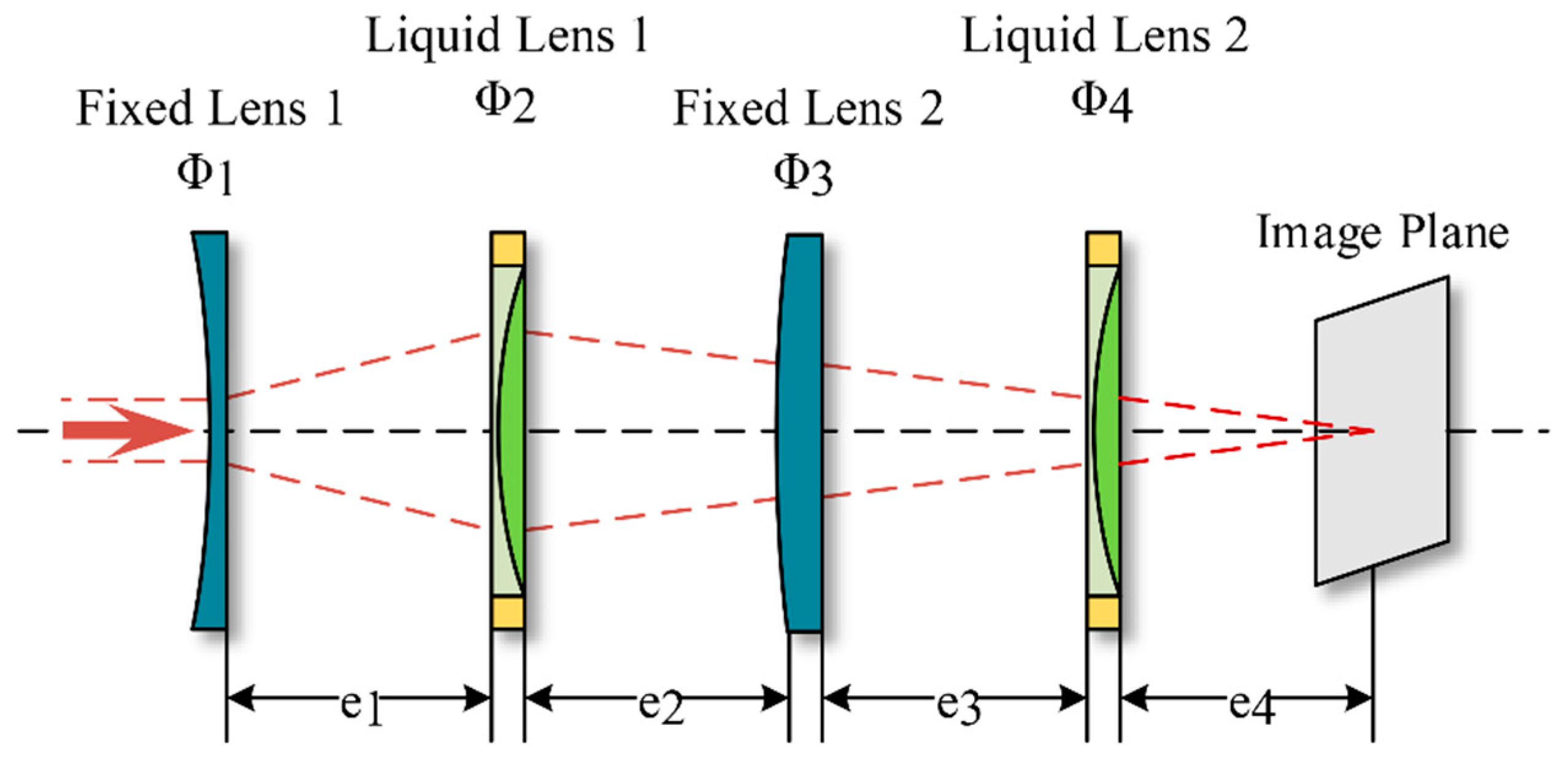
We presented a design method that is applicable to four-group stabilized zoom system in the previous work [18]. The optical layout of the four-group stabilized zoom system is shown in Figure 1, where Φ₁ and Φ₃ are the optical power of the fixed groups, Φ₂ and Φ₄ are optical power of the stabilized focal-length-variable groups. The terms e₁, e₂, e₃ are the separations between the consecutive principle planes in each group, e₄ is the separation between the last group and the image plane, m_i is magnification of each group.

Figure 1. Structure of the zoom system.

Figure 1. Structure of the zoom system.

In previous work, we analyzed this four-group stabilized zoom systems using the optical power of the optical element as the independent variables in the zoom equation. Simplified differential function is used to describe the relationship between the focal length variation of varifocal elements and the focal length variation of zoom system. The differentiable condition optimization can be used to get the analytic solution. In the zooming process, the function of the optical power of the focal length variable groups is monotonic, and the function of magnification has a breakpoint. The optical layout can be miniaturized as magnification has a larger derivative near the breakpoint. If the sign of m₃ is changeable during zooming, a larger derivative of m₃ can be found near the breakpoint. Then we optimize the Gaussian parameters of the fixed lens groups, make $\frac{e_4}{(1-e_1{\varphi }_1)\cdot {{ }^{2}B}_4}$ and $\frac{1-e_1{\varphi }_1}{e_4\cdot {{ }^{2}B}_4}$ (${}^{2}B_4=\left[-e_2,{\varphi }_3,-e_3\right]=e_2\cdot e_3\cdot {\varphi }_3-e_2-e_3$ is Gaussian brackets parameter) converge to a minimum to reach the requirement of zoom ratio.

In this paper, the optical design of a 5:1 stabilized zoom system is investigated. The zoom range is designed to be 7 mm to 35 mm. Design parameters are determined based on the requirement of a kind of ground vehicle being deployed on a bumpy road. The values of the Gaussian parameters are listed in Table 1, $\left|\frac{e_4}{(1-e_1{\varphi }_1)\cdot {{ }^{2}B}_4}\right|=0.12$, and $\left|\frac{1-e_1{\varphi }_1}{e_4\cdot {{ }^{2}B}_4}\right|=0.001$.

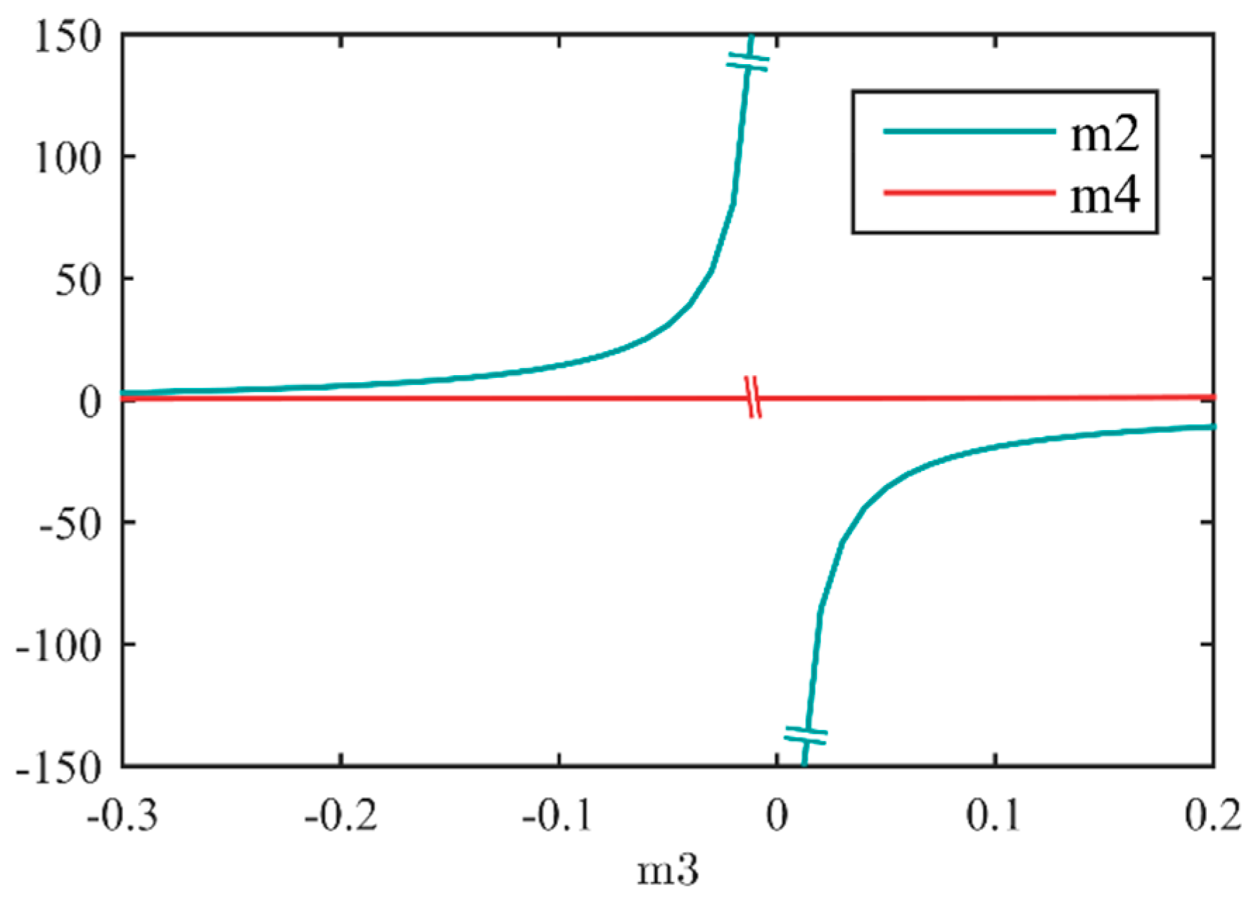
The relationship between m₂, m₃ and m₄ is shown in Figure 2, a larger derivative of m₃ can be found near the breakpoint since the sign of m₃ is changeable.

Table 1. Gaussian parameters of the zoom system.

	1/Φ (mm)	Φ2 (mm−1)	Φ4 (mm−1)	m2	m3	m4
Wide	7.27	0.008	0.019	1.28	−0.28	0.56
Middle	26.14	0.019	0	2.31	0.11	1.03
Tele	36.34	0.02	−0.01	2.53	0.19	1.24

Table 1. Gaussian parameters of the zoom system.

	1/Φ (mm)	Φ2 (mm−1)	Φ4 (mm−1)	m2	m3	m4
Wide	7.27	0.008	0.019	1.28	−0.28	0.56
Middle	26.14	0.019	0	2.31	0.11	1.03
Tele	36.34	0.02	−0.01	2.53	0.19	1.24

Figure 2. Relationship between m₂, m₃, and m₄. A larger derivative of m₃ can be found near the breakpoint since the sign of m₃ is changeable.

Figure 2. Relationship between m₂, m₃, and m₄. A larger derivative of m₃ can be found near the breakpoint since the sign of m₃ is changeable.

We use two liquid lenses (L₁ and L₂) as the focal length variable groups (Φ₂, Φ₄), the variation of Φ₂ and Φ₄ can be obtained as follows:

$${\mathsf{\Phi }}_2=\frac{e_4\mathsf{\Phi }-[{\varphi }_1,-(e_1+e_2),{\varphi }_3,-e_3]}{(1-e_1{\varphi }_1)\cdot {{ }^{2}B}_4}$$

(1)

$${\mathsf{\Phi }}_4=\frac{1-e_1{\varphi }_1}{e_4\mathsf{\Phi }\cdot {{ }^{2}B}_4}+\frac{{{ }^{2}B}_4-e_4[-e_2,{\varphi }_3]}{e_4\cdot {{ }^{2}B}_4}$$

(2)

$$\Delta {\mathsf{\Phi }}_2=\frac{e_4}{(1-e_1{\varphi }_1)\cdot {{ }^{2}B}_4}\Delta \mathsf{\Phi }$$

(3)

$$\Delta {\mathsf{\Phi }}_4=\frac{1-e_1{\varphi }_1}{e_4\cdot {{ }^{2}B}_4}\Delta \left(\frac{1}{\mathsf{\Phi }}\right)$$

(4)

where $\Delta \mathsf{\Phi }={\mathsf{\Phi }}_s-{\mathsf{\Phi }}_l$ is the variation of the system optical power, $\Delta \left(\frac{1}{\mathsf{\Phi }}\right)=\frac{1}{{\mathsf{\Phi }}_s}-\frac{1}{{\mathsf{\Phi }}_l}$, Φ_s and Φ_l represent the system optical power at the wide-angle end and the telephoto end respectively, ∆Φ₂ and ∆Φ₄ are the variation needed to achieve a given zoom range $\frac{1}{{\mathsf{\Phi }}_s}$ to $\frac{1}{{\mathsf{\Phi }}_l}$.

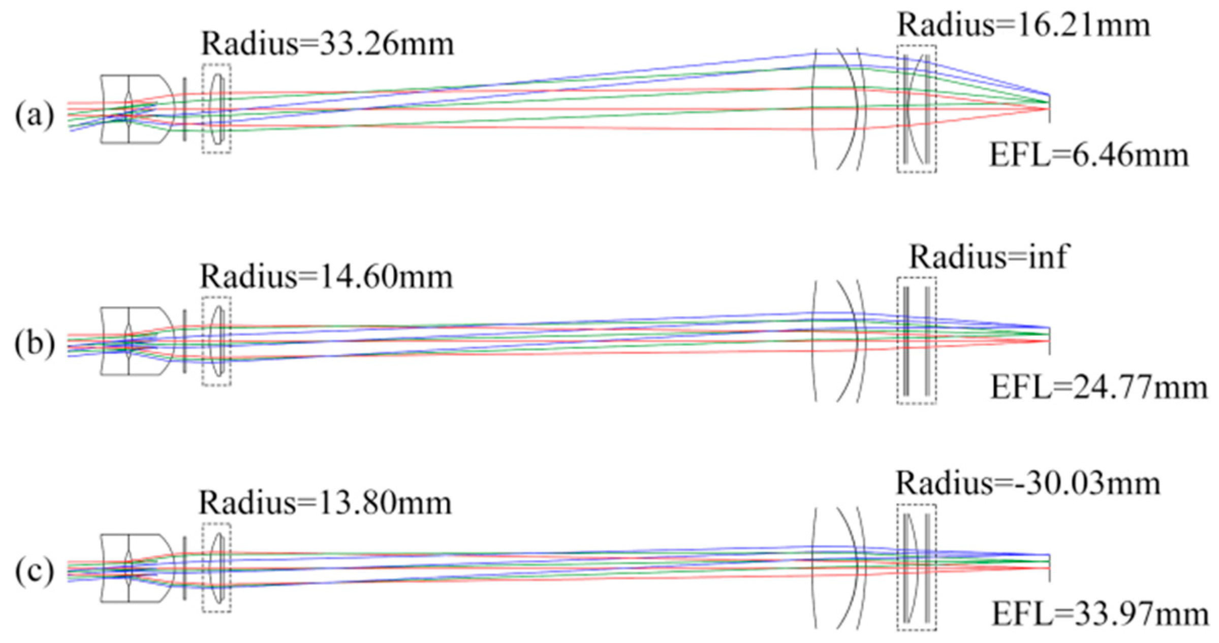
The general parameters of the zoom system are shown in Table 2. The initial lens structure of the optical system using these Gaussian parameters is simulated and optimized with the commercial optical design software named CODE V (Optical Research Associates, Tucson, AZ, USA), the result is shown in Figure 3, as the wide-angle end, the middle phase, and the telephoto end are shown in (a), (b), and (c), respectively.

Figure 3. Initial lens structure of the optical system.

Figure 3. Initial lens structure of the optical system.

Table 2. General parameters of the zoom system.

Surface	#	Curvature Radius	Thickness	Glass
Object		Infinity	Infinity
	1	Infinity	−9.7160
Fixed Lens1	2	−27.4979	3.7885	HLAF4_CDGM
	3	7.5970	1.4003
	4	−9.0978	7.8405	ZK9_CHINA
	5	−8.1539	1.5000
	6	Infinity	0.1000
Liquid Lens1	7	Infinity	0.5000	BK7_SCHOTT
	8	Infinity	zoom
	9	zoom	zoom	“OL1024”
	10	Infinity	0.5000	BK7_SCHOTT
	11	Infinity	1.1000
	12	Infinity	25.9971
	13	Infinity	81.4883
Fixed Lens2	14	77.7631	8.2500	ZK9_CHINA
	15	−18.8293	0.1000
	16	−18.5589	1.5000	ZF50_CDGM
	17	−41.6000	7.0723
	18	Infinity	0.0500
Liquid Lens2	19	Infinity	0.5000	BK7_SCHOTT
	20	Infinity	zoom
	21	zoom	zoom	“OL1024”
	22	Infinity	0.5000	BK7_SCHOTT
	23	Infinity	3.4500
	24	Infinity	0.8943
	25	Infinity	17.9482
Image		Infinity	0.0000

Table 2. General parameters of the zoom system.

Surface	#	Curvature Radius	Thickness	Glass
Object		Infinity	Infinity
	1	Infinity	−9.7160
Fixed Lens1	2	−27.4979	3.7885	HLAF4_CDGM
	3	7.5970	1.4003
	4	−9.0978	7.8405	ZK9_CHINA
	5	−8.1539	1.5000
	6	Infinity	0.1000
Liquid Lens1	7	Infinity	0.5000	BK7_SCHOTT
	8	Infinity	zoom
	9	zoom	zoom	“OL1024”
	10	Infinity	0.5000	BK7_SCHOTT
	11	Infinity	1.1000
	12	Infinity	25.9971
	13	Infinity	81.4883
Fixed Lens2	14	77.7631	8.2500	ZK9_CHINA
	15	−18.8293	0.1000
	16	−18.5589	1.5000	ZF50_CDGM
	17	−41.6000	7.0723
	18	Infinity	0.0500
Liquid Lens2	19	Infinity	0.5000	BK7_SCHOTT
	20	Infinity	zoom
	21	zoom	zoom	“OL1024”
	22	Infinity	0.5000	BK7_SCHOTT
	23	Infinity	3.4500
	24	Infinity	0.8943
	25	Infinity	17.9482
Image		Infinity	0.0000

2.2. Operating Range and Precision

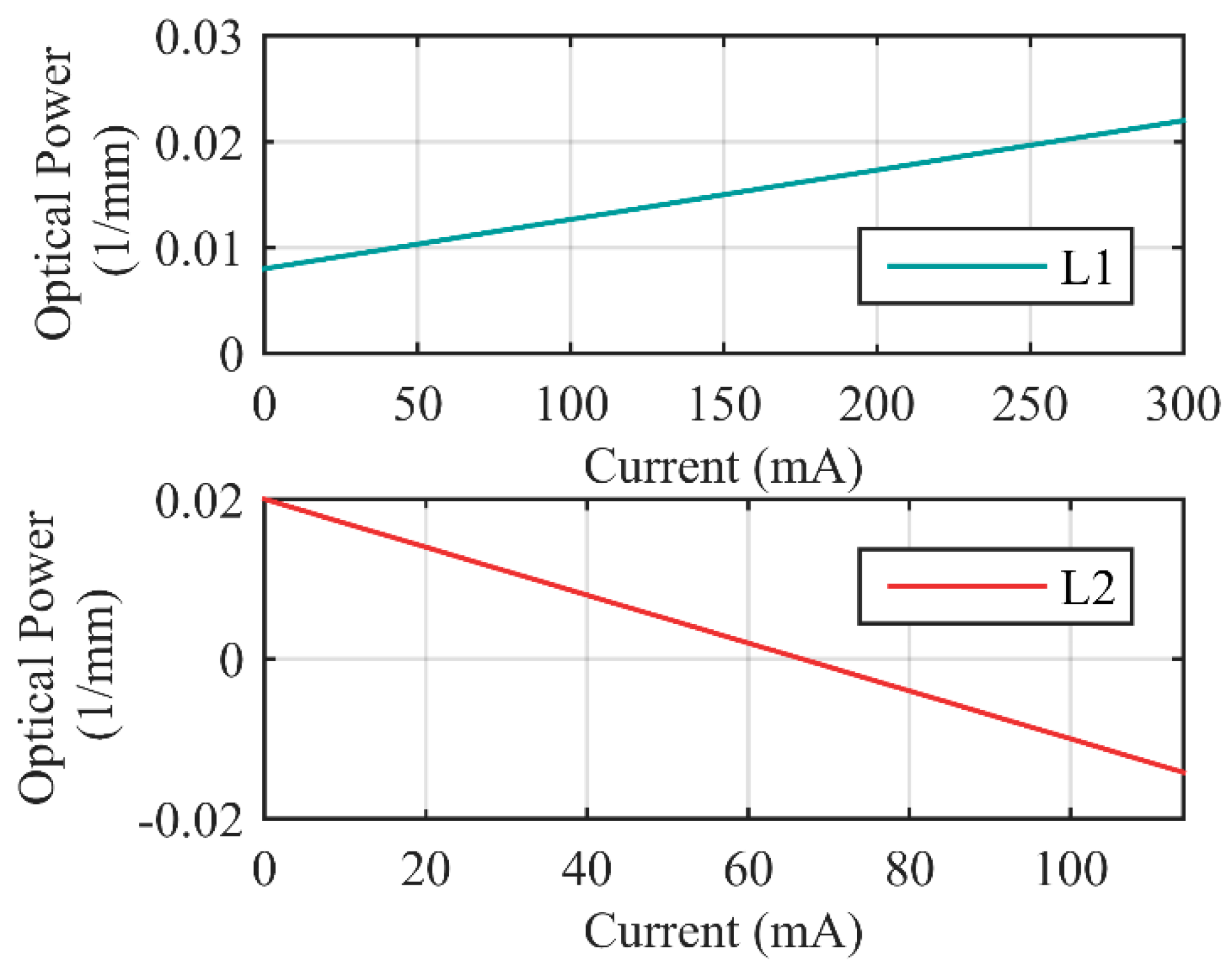
The zoom system operates by changing the optical power of two liquid lenses (L₁’s optical power Φ₂, and L₂’s optical power Φ₄). Two focus tunable lenses (Optotune, Swizerland) are used in the experiments, a 10 mm aperture commercial lens EL-10-30 for L₁, and a 20 mm aperture custom-design lens for L₂. Both L₁ and L₂ are liquid-filled membrane lenses, the refractive index of the lenses is 1.30, and Abbe number is 100. Φ₂ and Φ₄ are controlled by adjusting L₁’s control current (I₁) and L₂’s control current (I₂), respectively. Range of Φ₂ is 0.008 mm⁻¹ to 0.022 mm⁻¹, control precision is 4.67 × 10⁻⁵ mm⁻¹. Range of Φ₄ is −0.0142 mm⁻¹ to 0.02 mm⁻¹, the control precision is 3 × 10⁻⁴ mm⁻¹, zero optical power is attainable. The relationships between optical power and control currents are shown in Figure 4. As shown in figure, precision of L₁ is much higher than L₂, thus we use L₂ as active element, and use L₁ as servo element to compensate the image displacement.

Figure 4. Optical power of the liquid lenses as functions of control currents.

Figure 4. Optical power of the liquid lenses as functions of control currents.

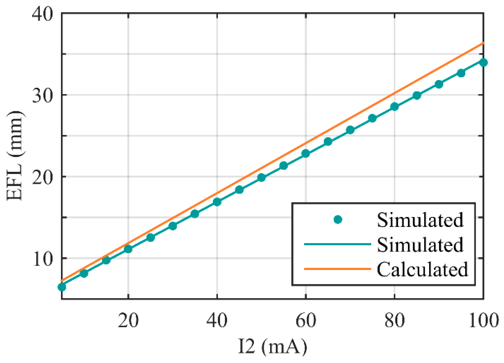
Our purpose is to design a zoom system with effective focal length (EFL) of 7 mm to 35 mm. In Section 2.1, we calculated the Gaussian parameters of the system, and optimized the system with CODE V. From Equation (2), we can calculate EFL of the zoom system theoretically. The calculated range of EFL is 7.27 mm to 36.34 mm, the zoom ratio is 5:1. Then we simulate the designed system, select 20 sampling points, set I₂ from 5 mA to 100 mA, respectively. Relationships between EFL and I₂ are shown in Figure 5. The simulated EFL range is 6.46 mm to 33.97 mm, and the zoom ratio is 5.26:1.

Figure 5. Calculated and simulated EFL as functions of I₂. The “simulated dots” mark the EFL of sampling points that be obtained by CODE V. The “simulated line” is the fitting curve of the dots.

Figure 5. Calculated and simulated EFL as functions of I₂. The “simulated dots” mark the EFL of sampling points that be obtained by CODE V. The “simulated line” is the fitting curve of the dots.

In this paper, zoom precision is defined as the minimum variation of EFL that can be adjusted i.e., the variation of EFL when I₂ increase or decrease 1 mA. From Equation (4), we can theoretically calculate the zoom precision to be 0.3 mm. Then we simulate the zoom precision with CODE V. We firstly select 20 sampling points when I₂ takes different values listed in Table 3, then make I₂ increase 1 mA, corresponding values of Φ₄ can be obtained from Figure 4. The simulated results are shown in Table 3.

Table 3. Simulated zoom precision of the zoom system.

I2 (mA)	Zoom Precision (mm)	I2 (mA)	Zoom Precision (mm)
5	0.2911	55	0.2945
10	0.2731	60	0.2924
15	0.2612	65	0.2898
20	0.2762	70	0.2867
25	0.2862	75	0.2832
30	0.292	80	0.2792
35	0.295	85	0.2749
40	0.2964	90	0.2703
45	0.2966	95	0.2652
50	0.2959	100	0.2601
Average	0.2830	RMS	0.0122

Table 3. Simulated zoom precision of the zoom system.

I2 (mA)	Zoom Precision (mm)	I2 (mA)	Zoom Precision (mm)
5	0.2911	55	0.2945
10	0.2731	60	0.2924
15	0.2612	65	0.2898
20	0.2762	70	0.2867
25	0.2862	75	0.2832
30	0.292	80	0.2792
35	0.295	85	0.2749
40	0.2964	90	0.2703
45	0.2966	95	0.2652
50	0.2959	100	0.2601
Average	0.2830	RMS	0.0122

Therefore, we designed and simulated a zoom system with 5:1 zoom ratio. The calculated EFL range is 7.27 mm to 36.34 mm while the simulated range is 6.46 mm to 33.97 mm. The calculated zoom precision is 0.3 mm while the average simulated value is 0.2830, and root-mean-square (RMS) of the simulated zoom precision is 0.0122 mm.

3. Experimental and Analysis

3.1. Experimental Setup

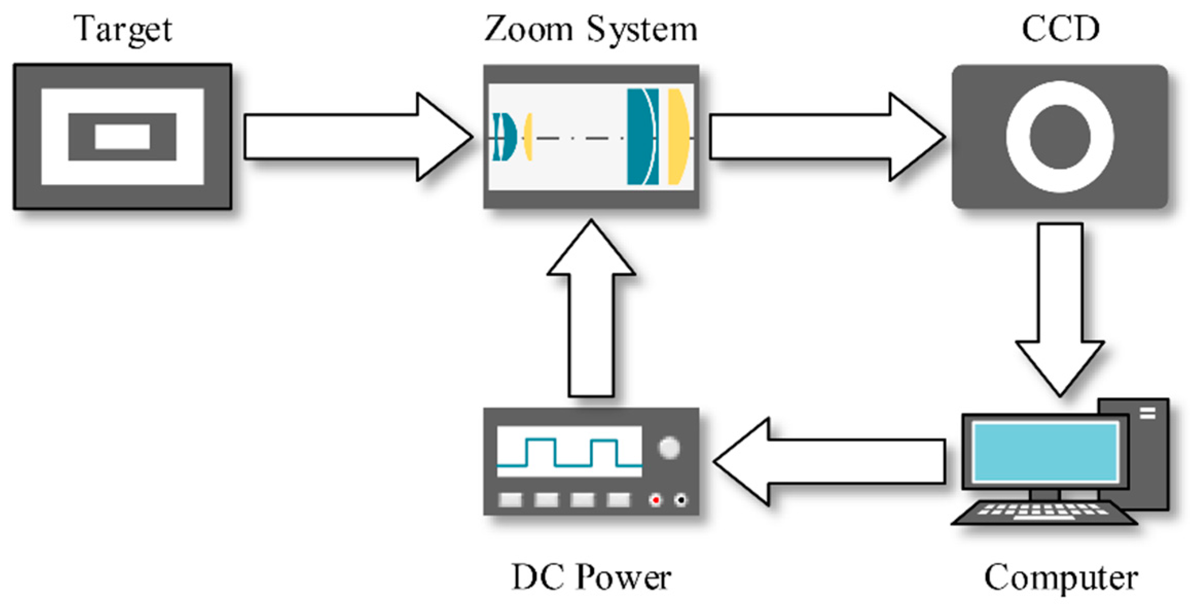
In order to test the performance of the zoom system, we set up an experimental platform shown in Figure 6. Test targets were backlit with white light and two forms of targets were used in measurement. The size of the target was 240 mm × 170 mm. The zoom system was placed between the test target and the CCD camera, and the object distance was set to be 265 mm. The CCD was 1/4 inch, pixel size of which was 7.4 μm. In fact, the zoom system and the CCD camera were fixed connected through a standard C lens mount. CCD camera captured the images and then sent them to the computer. We obtained the information on imaging quality and magnification through image processing, and then sent new control parameters to the zoom system. A dc power supply was used to complete the D/A conversion.

Figure 6. Structure of the experimental platform.

Figure 6. Structure of the experimental platform.

There were two major parameters we needed to measure: EFL and modulation transfer function (MTF). EFL was used to evaluate the zoom ratio and zoom precision, and MTF was used to evaluate the imaging quality. During measurement, we selected 20 sampling points as we had done in simulation when adjusted I₂ from 5 mA to 100 mA. The forms of targets and the methods of measuring EFL and MTF would be discussed in the following sections.

3.2. Initial Structure

In their initial state, I₁ and I₂ both took 0 mA. MTF was used to evaluate the quality of imaging. The method of calculating MTF of the system would be provided in Section 3.6, we currently used the calculation result. Initial parameters of the zoom system are shown in Table 4. MTF value when spatial frequency took 20 lp/mm was used to evaluate the image quality.

Table 4. Initial parameters of the zoom system.

I2 (mA)	EFL (mm)	FOV (Degree)	MTF Value at 20l p/mm
0	6.56	41.7	0.01
5	6.93	39.7	0.28

Table 4. Initial parameters of the zoom system.

I2 (mA)	EFL (mm)	FOV (Degree)	MTF Value at 20l p/mm
0	6.56	41.7	0.01
5	6.93	39.7	0.28

Image quality was poor because L₁ had not compensated for L₂ and the optical aberration of L₂ was high when Φ₄ took values near the limit position.

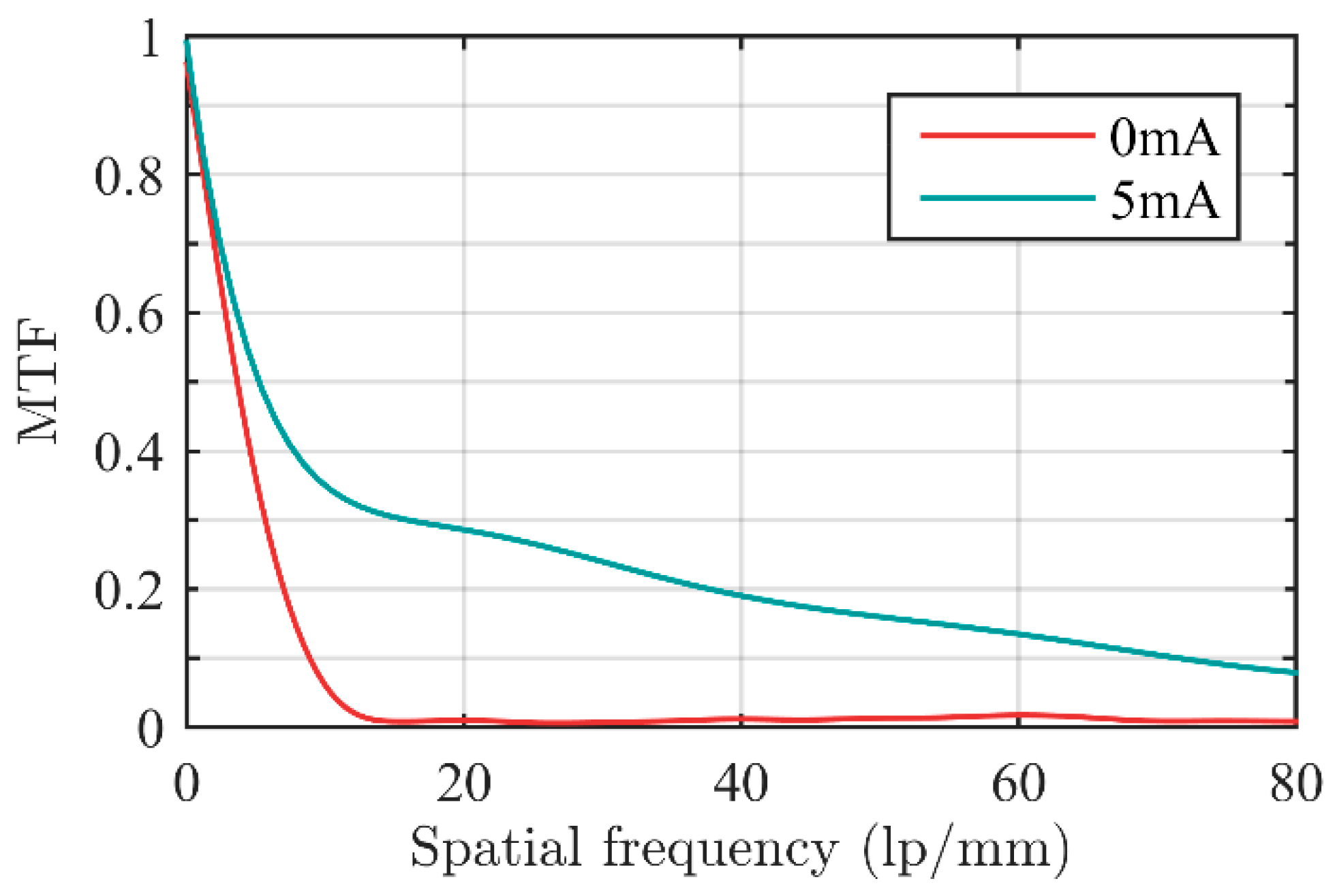
In order to achieve high image quality in the whole zoom process, we set I₂ = 5 mA and adjusted L₁ to compensate for L₂. MTF diagram is shown in Figure 7. Parameters of the zoom system when I₂ takes 5 mA are shown in Table 4.

Figure 7. MTF curve of the zoom system when I₂ took 0 mA and 5 mA, respectively.

Figure 7. MTF curve of the zoom system when I₂ took 0 mA and 5 mA, respectively.

In the following discussion, we take the state when I₂ = 5 mA as the initial state.

3.3. Electrical Performance Testing

In the process of measuring, L₂ was adjusted actively to change EFL of the zoom system when L₁ supplied compensation to get clear images. The relationship between I₁ and I₂ can be calculated from Equations (1) and (2).

We set I₂ to a value, coarsely adjusted I₁ till we got clear image on computer, and then tightly adjusted I₁. Range of tight adjustment was usually less than ±4 mA in actual measurement. We could obtain the real-time MTF of the zoom system with the software written by ourselves on computer. In fact, the MTF curve had no obvious change when we adjusted I₁ in ±2 mA range. For I₁, this was an acceptable error range. Then we chose the value of MTF when spatial frequency was 20l p/mm as the image quality factor (Q). We considered the zoom system to achieve highest imaging quality when Q got maximum, and I₁ would be recorded. The results of simulation and measurement are shown in Figure 8. Although there were differences between simulated curve and measured curve, we could easily obtain I₁ as function of I₂ by curve fitting. This enabled the zoom system to realize precise electric control. Both the simulated and the measured curves could be fitted well by three-order polynomials, and the correlation coefficients were larger than 0.999. This meant that we only needed a small amount of addition and multiplication operations to obtain I₁ by I₂.

Figure 8. L₁’s control current (I₁) as function of L₂’s control current (I₂).

Figure 8. L₁’s control current (I₁) as function of L₂’s control current (I₂).

Optical power of the liquid lens was the only variant in the zoom system. Although in actual application on ground vehicle, it needed time to calculate I₁ and I₂ for specific EFL, the calculation time was usually at a microsecond level for most of the processors since there were only multiply and add operations in the fitting function. Therefore, the zoom speed depended only on the performance of the liquid lens. The response time of the system was less than 2.5 ms, and the settling time was less than 15 ms due to fluid viscosity.

3.4. Zoom Ratio Testing

Relationships between EFL, field of view (FOV), object height (OH), paraxial image height (PIH), and object distance (OD) could be obtained refer to Equations (5) and (6).

$$PIH=EFL\cdot \tan (\frac{1}{2}FOV)$$

(5)

$$OH=OD\cdot \tan (\frac{1}{2}FOV)$$

(6)

We obtained the magnification (m) of the zoom system by imaging a fixed length (l_o) target. The magnification could be calculated refer to Equation (7) by counting the pixels (n) when the pixel size (μ) of the CCD camera was known.

$$m=n\cdot \mu /l_o=PIH/OH$$

(7)

Thus from Equations (5)−(7), we can obtain EFL refer to Equation (8).

$$EFL=m\cdot OD$$

(8)

The measured and simulated results of EFLs are shown in Table 5, and the EFL comparison diagram of calculated value, simulated value and measured value is shown in Figure 9. An approximate linear relationship exists between EFL and I₂. Thus, we can easily determine I₂ to achieve specific EFL in actual application. As presented in Section 3.3, I₁ could be calculated out by I₂ through the fitting function. Thus far, issues of determining control parameters to achieve specific EFL are completely solved.

Table 5. Comparisons between simulated EFL and measured EFL.

I2 (mA)	Simulated EFL (mm)	Measured EFL (mm)	Difference (mm)
5	6.46	6.93	0.47
10	8.14	7.81	−0.33
15	9.78	8.58	−1.20
20	11.12	9.77	−1.35
25	12.52	10.85	−1.67
30	13.97	12.15	−1.82
35	15.43	13.38	−2.05
40	16.91	14.80	−2.11
45	18.39	16.28	−2.11
50	19.88	17.95	−1.93
55	21.35	19.67	−1.68
60	22.82	21.40	−1.42
65	24.28	23.19	−1.09
70	25.72	24.91	−0.81
75	27.15	26.7	−0.45
80	28.56	28.55	0.01
85	29.94	30.77	0.83
90	31.31	32.31	1.00
95	32.65	33.46	0.81
100	33.97	35.06	1.09

Table 5. Comparisons between simulated EFL and measured EFL.

I2 (mA)	Simulated EFL (mm)	Measured EFL (mm)	Difference (mm)
5	6.46	6.93	0.47
10	8.14	7.81	−0.33
15	9.78	8.58	−1.20
20	11.12	9.77	−1.35
25	12.52	10.85	−1.67
30	13.97	12.15	−1.82
35	15.43	13.38	−2.05
40	16.91	14.80	−2.11
45	18.39	16.28	−2.11
50	19.88	17.95	−1.93
55	21.35	19.67	−1.68
60	22.82	21.40	−1.42
65	24.28	23.19	−1.09
70	25.72	24.91	−0.81
75	27.15	26.7	−0.45
80	28.56	28.55	0.01
85	29.94	30.77	0.83
90	31.31	32.31	1.00
95	32.65	33.46	0.81
100	33.97	35.06	1.09

Figure 9. EFL comparison among calculated value, simulated value, and measured value.

Figure 9. EFL comparison among calculated value, simulated value, and measured value.

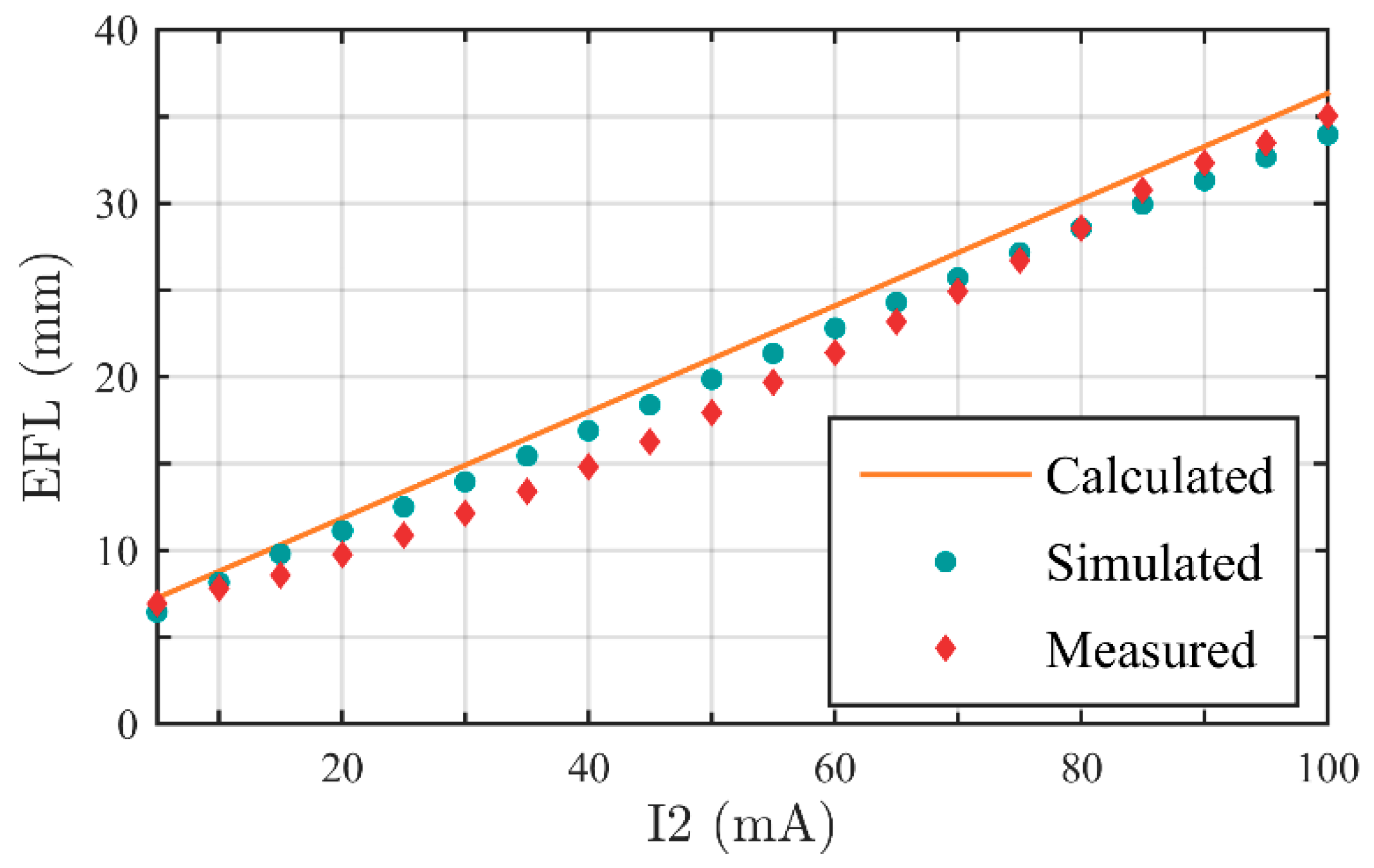
Therefore, the measured EFL range of the zoom system is 6.93 mm to 35.06 mm, the zoom ratio is 5.06:1. When I₂ = 5 mA, EFL takes minimum, at this moment Φ₂ = 0.0087 mm⁻¹ and Φ₄ = 0.0185 mm⁻¹, the FOV is 40°. When I₂ = 100 mA, EFL takes maximum, Φ₂ = 0.0192 mm⁻¹ and Φ₄ = −0.0100 mm⁻¹ at this moment, the FOV is 8°.

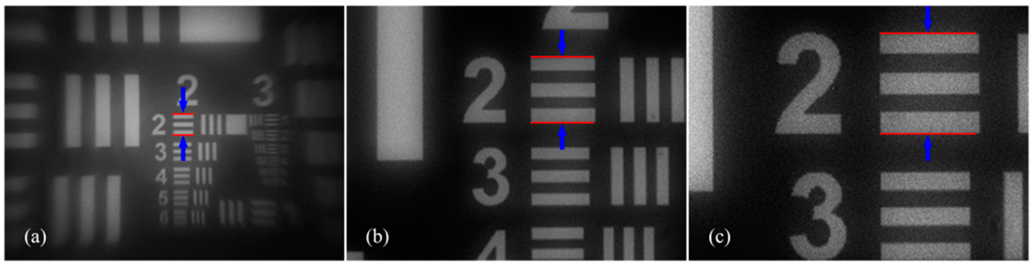
Images captured in different EFL are shown in Figure 10a–c show the wide end, the middle phase, and the tele end respectively. In wide end, EFL is 6.93 mm, the zoom system has the widest FOV, and there are 18 pixels between two red lines shown in Figure 10a. In tele end, EFL is 35.06 mm, the zoom system is most detailed, and the number of pixels between two red lines shown in Figure 10c increases to 91. We can also get the conclusion of a 5.06:1 zoom ratio. A middle phase is presented too, in order to make readers observe the zoom process from wide end to tele end visually.

Figure 10. Images captured in different EFL. (a) wide end, when I₂ = 5 mA, 18 pixels between two red lines; (b) middle phase, when I₂ = 60 mA, 59 pixels between two red lines; (c) tele end, when I₂ = 100 mA, 91 pixels between two red lines.

Figure 10. Images captured in different EFL. (a) wide end, when I₂ = 5 mA, 18 pixels between two red lines; (b) middle phase, when I₂ = 60 mA, 59 pixels between two red lines; (c) tele end, when I₂ = 100 mA, 91 pixels between two red lines.

3.5. Zoom Precision Testing

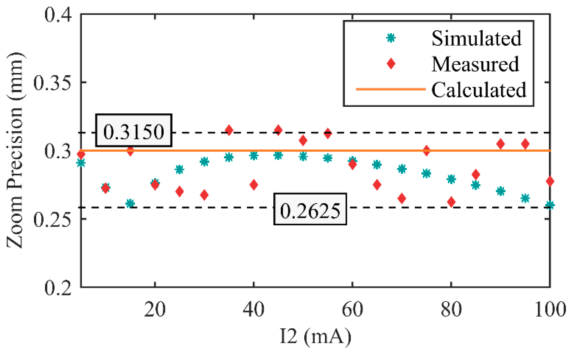
In order to measure the zoom precision of the system, we set I₂ to a value firstly, measured EFL at this moment. Then we adjusted I₂ to increase 1 mA, and measured the variation of EFL. In the above, we had simulated the test process. The simulated results had been shown in Table 3. The measured results are shown in Table 6, and diagram of comparison among calculated, simulated, and measured results is shown in Figure 11.

Table 6. Measured zoom precision.

I2 (mA)	Zoom Precision (mm)	I2 (mA)	Zoom Precision (mm)
5	0.2975	55	0.3125
10	0.2725	60	0.2900
15	0.3000	65	0.2750
20	0.2750	70	0.2650
25	0.2700	75	0.3000
30	0.2675	80	0.2625
35	0.3150	85	0.2825
40	0.2750	90	0.3050
45	0.3150	95	0.3050
50	0.3075	100	0.2775
Average	0.2885	RMS	0.0181

Table 6. Measured zoom precision.

I2 (mA)	Zoom Precision (mm)	I2 (mA)	Zoom Precision (mm)
5	0.2975	55	0.3125
10	0.2725	60	0.2900
15	0.3000	65	0.2750
20	0.2750	70	0.2650
25	0.2700	75	0.3000
30	0.2675	80	0.2625
35	0.3150	85	0.2825
40	0.2750	90	0.3050
45	0.3150	95	0.3050
50	0.3075	100	0.2775
Average	0.2885	RMS	0.0181

Figure 11. Zoom precision comparison among calculated, simulated, and measured values.

Figure 11. Zoom precision comparison among calculated, simulated, and measured values.

Zoom precision of the realized zoom system is approximately uniform in the whole zoom process. The average of measured zoom precision is 0.2885 mm, near to the calculated value 0.3 mm, and all of measured values are in the range of ±0.0265 mm to average zoom precision, RMS of the measured zoom precision is 0.0181 mm. Parameters of the realized lens are consistent with the calculated and simulated values.

Therefore, there are 96 discrete EFL states in the entire zoom range, spaces between adjacent states are approximately uniform to be 0.2885 mm. Because the EFL states are so compact, we can consider the realized system as a continuous zoom system.

3.6. Imaging Quality Testing

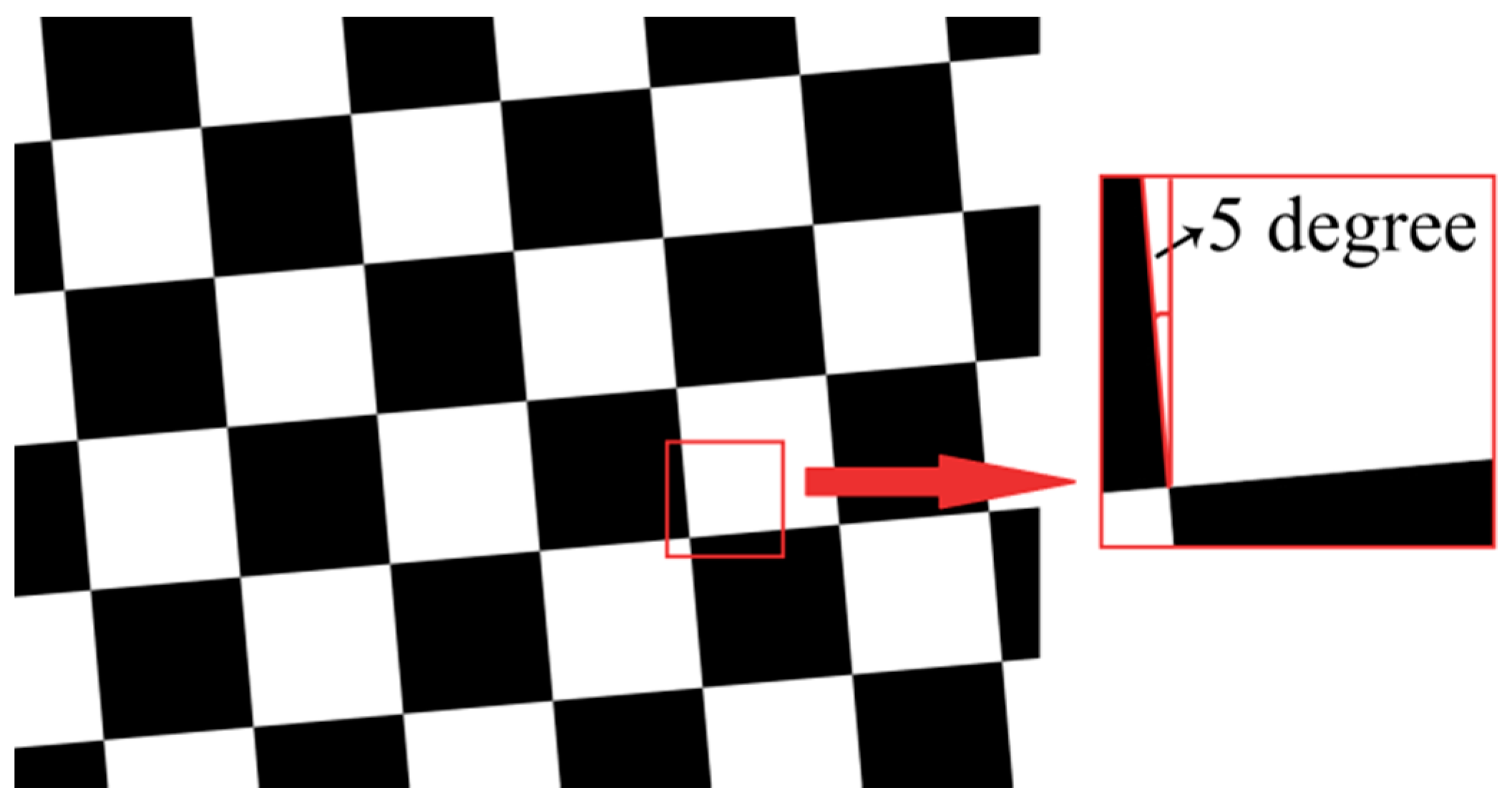
We used MTF to evaluate the imaging quality of the zoom system. The test target used in imaging quality testing is shown in Figure 12, similar to a black and white chessboard. The tilt of edge was set to 5° according to ISO12233.

Figure 12. Structure of the target used to test the imaging quality.

Figure 12. Structure of the target used to test the imaging quality.

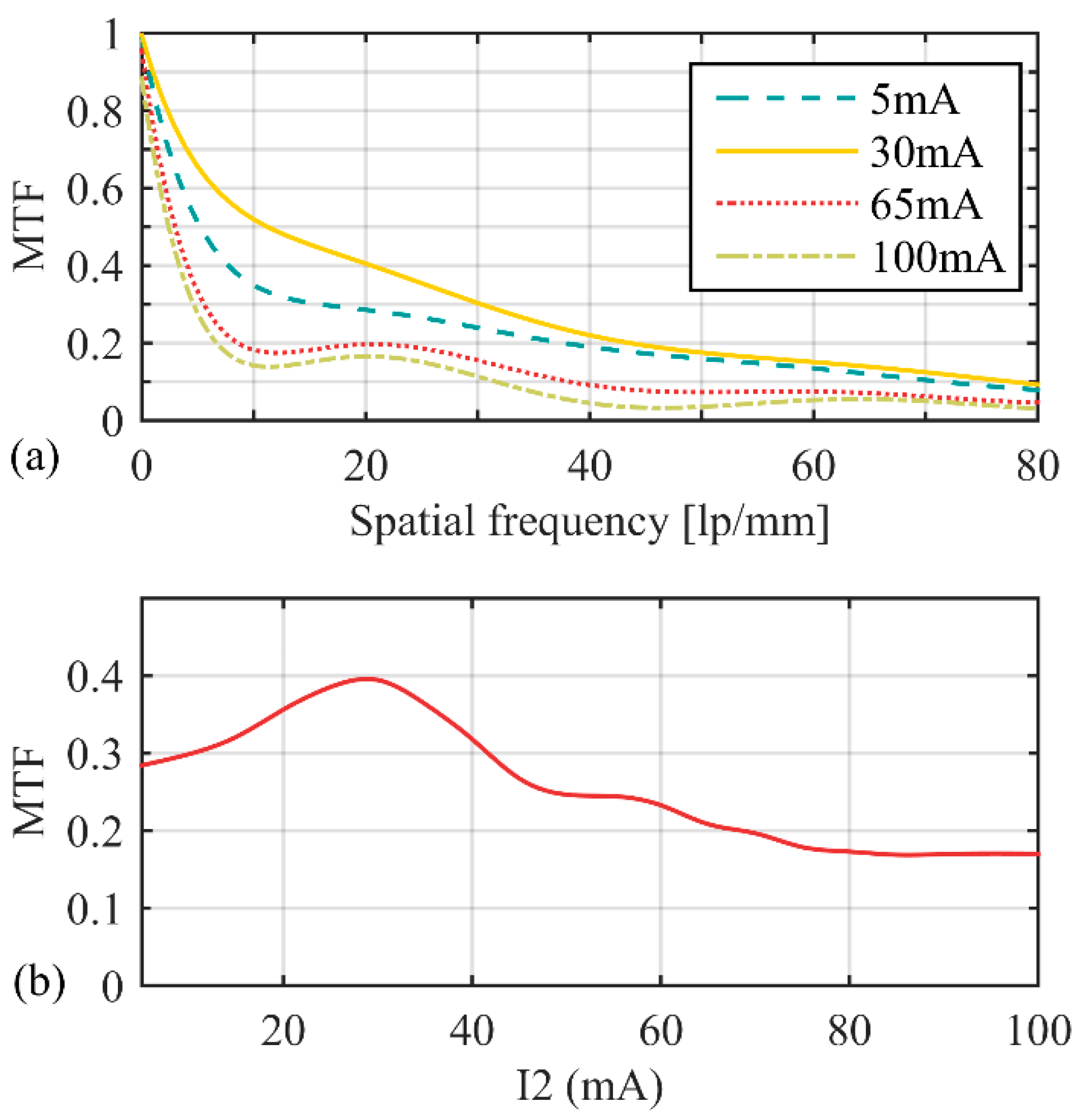
In the test process, we selected a region-of-interest (ROI) that contains a slanted-edge in the beginning, then obtained the Edge Spread Function (ESF) by the use of knife-edge method and got the Line Spread Function (LSF) through the differential of ESF. The MTF could be computed by a Fast Fourier Transform (FFT) of LSF. MTFs were measured when I₂ took different values. The results are shown in Figure 13a.

Figure 13. MTF of the zoom system. (a) MTFs were measured when I₂ took different values; (b) relationship between MTF and I₂ at 20 lp/mm.

Figure 13. MTF of the zoom system. (a) MTFs were measured when I₂ took different values; (b) relationship between MTF and I₂ at 20 lp/mm.

At 20 lp/mm, the relationship between MTF and I₂ is shown in Figure 13b. The zoom system got the highest imaging quality when I₂ = 30 mA, MTF reached 0.40 at 20 lp/mm. When I₂ > 90 mA, MTF reduced to 0.17 at 20 lp/mm.

4. Conclusions

In this paper, we designed and realized an electrically tunable four-group stabilized zoom system by using two liquid lenses. The zoom equations were established by using Gaussian bracket method. L₁ and L₂ were used as the second and the fourth lens group that were focal length variable. The calculated EFL range was 7.27 mm to 36.34 mm while the zoom precision was calculated to be 0.3 mm. We simulated the zoom system, got the simulated EFL range was 6.46 mm to 33.97 mm and the zoom precision was 0.283 mm. Then we made a series of experiments to verify the performance of the realized system. Response time of the realized zoom system was less than 2.5 ms, and the settling time was less than 15 ms. The measured EFL range was 6.93 mm to 35.06 mm, the zoom ratio was 5.06:1. When Φ₂ = 0.0087 mm⁻¹ and Φ₄ = 0.0185 mm⁻¹, EFL got the minimum value, the FOV was 40°. When Φ₂ = 0.0192 mm⁻¹ and Φ₄ = −0.01 mm⁻¹, EFL got the maximum value, the FOV was 8°. The measured EFL adjust precision was 0.2885 mm, the RMS of precision was 0.0181 mm. MTF was used to evaluate the imaging quality of the zoom system. The range of MTF was 0.17 to 0.40 at 20 lp/mm. The lens realized in this paper had only four groups of elements, and none of them was motorized, thus it had good anti-shake performance. It was applicable to many fields e.g., ground vehicles used in a field-environment, and was also suitable for applications in high speed vehicles and fast moving target tracking as a result of the good electrical performance.

However, the gravity influence of liquid lens was not considered in this paper. Although in the experiments, no apparent gravity effect had been observed, it would exist in theory. In fact, gravity effect in the stationary state had been contained in the parameter “wavefront error” in the datasheet of the liquid lens, the wavefront error was less than 0.5λ. In practice, we need to consider the system working in doubling even tripling gravitational acceleration environments. We will do more research on this issue in future works.

References

- Herzberger, M. Modern Geometrical Optics; Interscience Publishers, Inc.: New York, NY, USA, 1958. [Google Scholar]
- Lin, Y.H.; Chen, M.S. A pico projection system with electrically tunable optical zoom ratio adopting two liquid crystal lenses. J. Disp. Technol. 2012, 8, 401–404. [Google Scholar] [CrossRef]
- Foresti, G.L.; Micheloni, C.; Piciarelli, C.; Snidaro, L. Visual sensor technology for advanced surveillance systems: Historical view, technological aspects and research activities in Italy. Sensors 2009, 9, 2252–2270. [Google Scholar] [CrossRef] [PubMed]
- Zou, T.; Tang, X.; Song, B.; Wang, J.; Chen, J. Robust feedback zoom tracking for digital video surveillance. Sensors 2012, 12, 8073–8099. [Google Scholar] [CrossRef] [PubMed]
- Zhao, P.P.; Ataman, C.; Zappe, H. An endoscopic microscope with liquid-tunable aspheric lenses for continuous zoom capability. In Proceedings of the SPIE Micro-Optics 2014, Brussels, Belgium, 14–16 April 2014.
- Wick, D.V.; Martinez, T.; Payne, D.M.; Sweatt, W.C.; Restaino, S.R. Active optical zoom system. In Proceedings of the SPIE Conference on Spaceborne Sensors II, Orlando, FL, USA, 28–29 March 2005.
- Wick, D.V.; Martinez, T. Adaptive optical zoom. Opt. Eng. 2004, 43, 8–9. [Google Scholar]
- Ren, H.W.; Wu, S.T. Variable-focus liquid lens. Opt. Express 2007, 15, 5931–5936. [Google Scholar] [CrossRef] [PubMed]
- Lin, Y.S.; Chen, M.S.; Lin, H.C. An electrically tunable optical zoom system using two composite liquid crystal lenses with a large zoom ratio. Opt. Express 2001, 19, 4714–4721. [Google Scholar] [CrossRef] [PubMed]
- Zhang, W.; Tian, W. A novel micro zoom system design with liquid lens. In Proceedings of the 2008 International Conference on Optical Instruments and Technology—Optical Systems and Optoelectronic Instruments, Beijing, China, 16–19 November 2008.
- Peng, R.; Chen, J.; Zhu, C.; Zhuang, S. Design of a zoom lens without motorized optical elements. Opt. Express 2007, 15, 6664–6669. [Google Scholar] [CrossRef] [PubMed]
- Fang, Y.C.; Tsai, C.M.; Chung, C.L. A study of optical design and optimization of zoom optics with liquid lenses through modified genetic algorithm. Opt. Express 2011, 19, 16291–16302. [Google Scholar] [CrossRef] [PubMed]
- Miks, A.; Novak, J. Analysis of two-element zoom systems based on variable power lenses. Opt. Express 2010, 18, 6797–6810. [Google Scholar] [CrossRef] [PubMed]
- Park, S.C.; Lee, W.S. Design and analysis of a one-moving-group zoom system using a liquid lens. J. Korean Phys. Soc. 2013, 62, 435–442. [Google Scholar] [CrossRef]
- Peng, R.; Chen, J.; Zhuang, S. Electrowetting-actuated zoom lens with spherical-interface liquid lenses. J. Opt. Soc. Am. A 2008, 25, 2644–2650. [Google Scholar] [CrossRef]
- Sun, J.H.; Hsueh, B.R.; Fang, Y.C.; MacDonald, J.; Hu, C.C. Optical design and multiobjective optimization of miniature zoom optics with liquid lens element. Appl. Opt. 2009, 48, 1741–1757. [Google Scholar] [CrossRef] [PubMed]
- Zhang, W.; Li, D.; Guo, X. Optical Design and Optimization of a Micro Zoom System with Liquid Lenses. J. Opt. Soc. Korea 2013, 17, 447–453. [Google Scholar] [CrossRef]
- Hao, Q.; Cheng, X.; Du, K. Four-group stabilized zoom lens design of two focal-length-variable elements. Opt. Express 2013, 21, 7758–7767. [Google Scholar] [CrossRef] [PubMed]
© 2015 by the authors; licensee MDPI, Basel, Switzerland. This article is an open access article distributed under the terms and conditions of the Creative Commons by Attribution (CC-BY) license (http://creativecommons.org/licenses/by/4.0/).
Share and Cite
MDPI and ACS Style
Li, H.; Cheng, X.; Hao, Q. An Electrically Tunable Zoom System Using Liquid Lenses. Sensors 2016, 16, 45. https://doi.org/10.3390/s16010045
AMA Style
Li H, Cheng X, Hao Q. An Electrically Tunable Zoom System Using Liquid Lenses. Sensors. 2016; 16(1):45. https://doi.org/10.3390/s16010045
Chicago/Turabian StyleLi, Heng, Xuemin Cheng, and Qun Hao. 2016. "An Electrically Tunable Zoom System Using Liquid Lenses" Sensors 16, no. 1: 45. https://doi.org/10.3390/s16010045
Note that from the first issue of 2016, this journal uses article numbers instead of page numbers. See further details here.