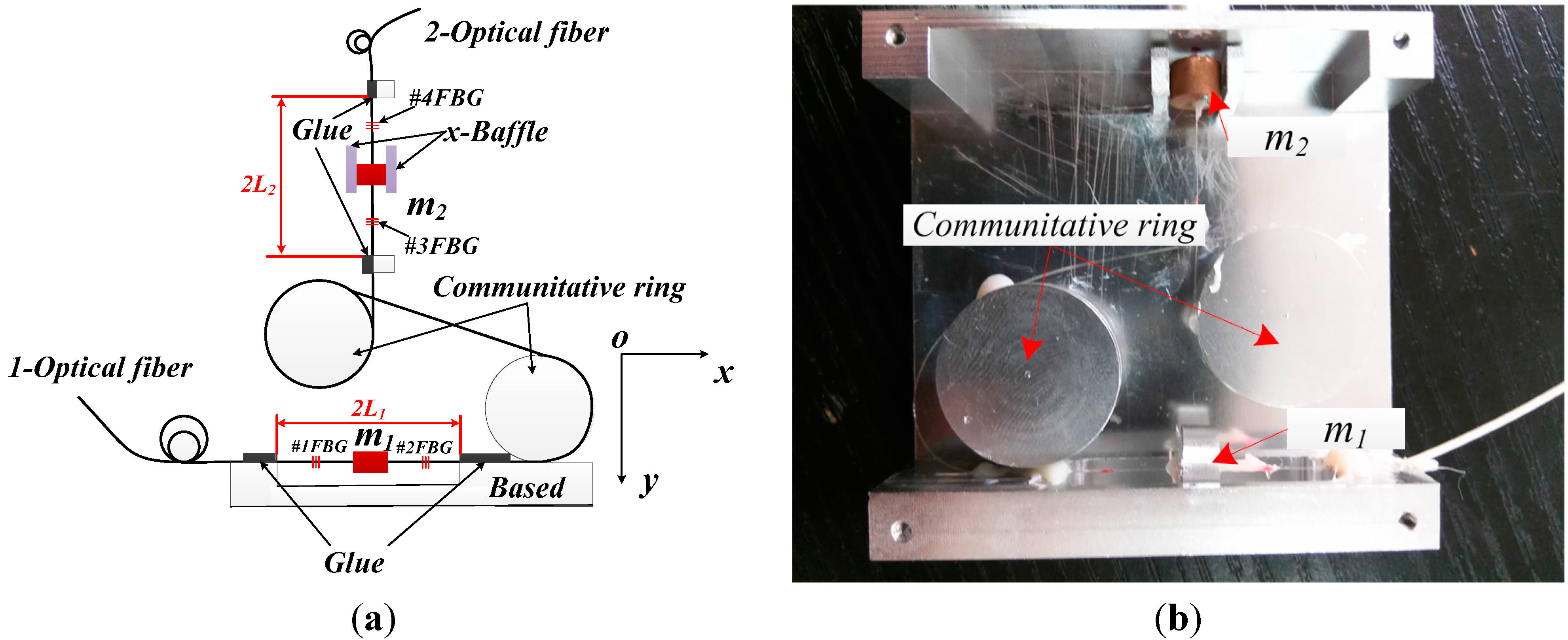
Figure 4.
Schematic diagram and photograph of sensing characteristics experiment.
3.1. Dynamic Characteristic Experiments of Sensor
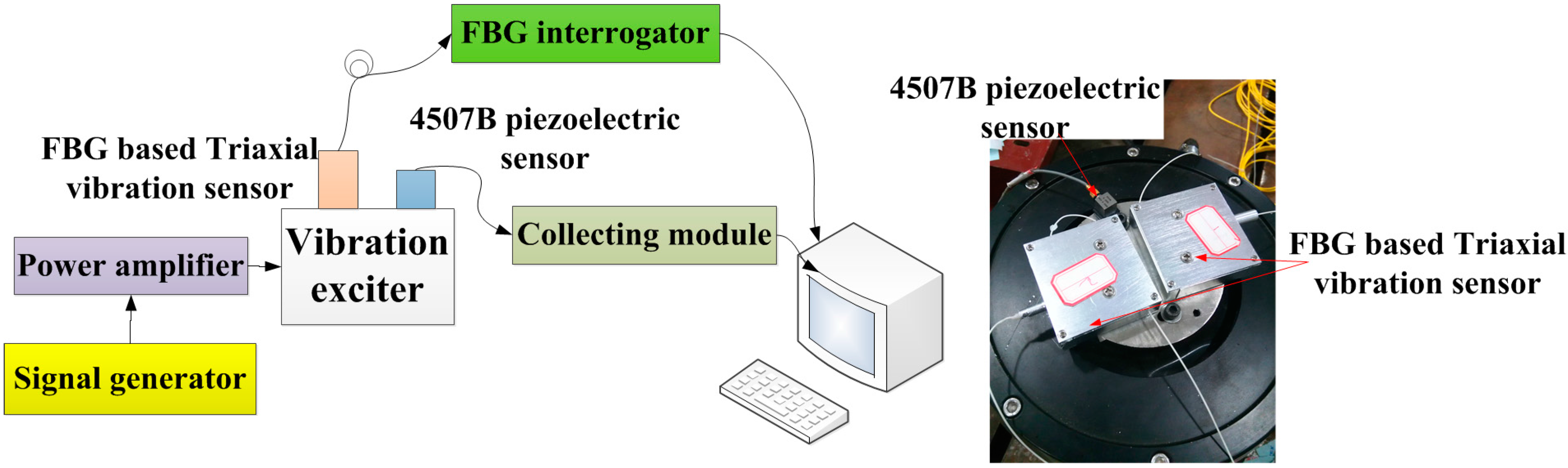
Dynamic property is one of the important indicators to evaluate performance of sensor. In order to investigate the dynamic properties, the sensor is fixed on the vibration exciter (
Figure 4), and the
x-direction is treated as the main vibration direction. During the experiment, the frequency of acceleration changes within 20 to 1000 Hz, and amplitude of acceleration is always kept at 10 m/s
2. In order to ensure repeatability of results, the experiment has been repeated three times. The
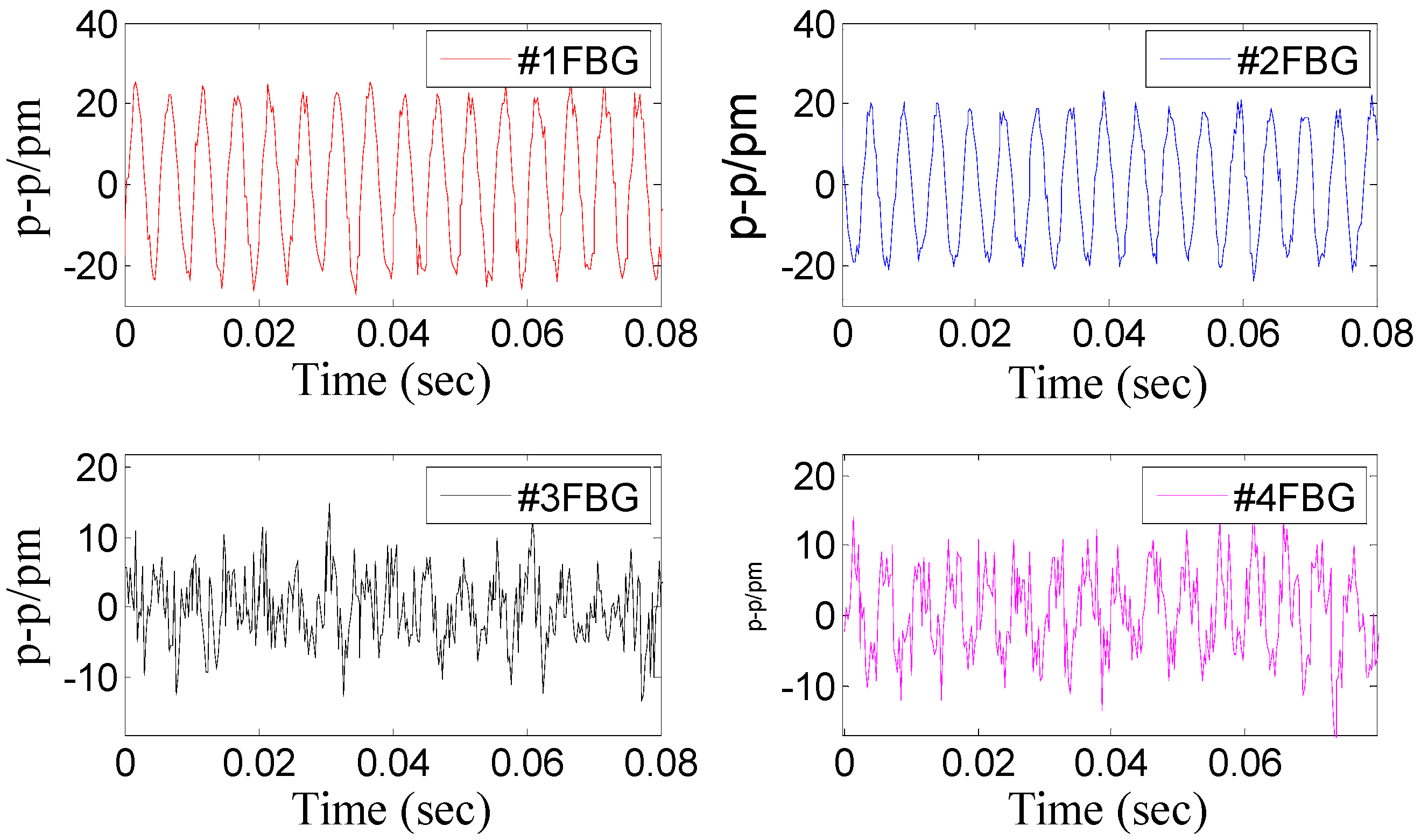
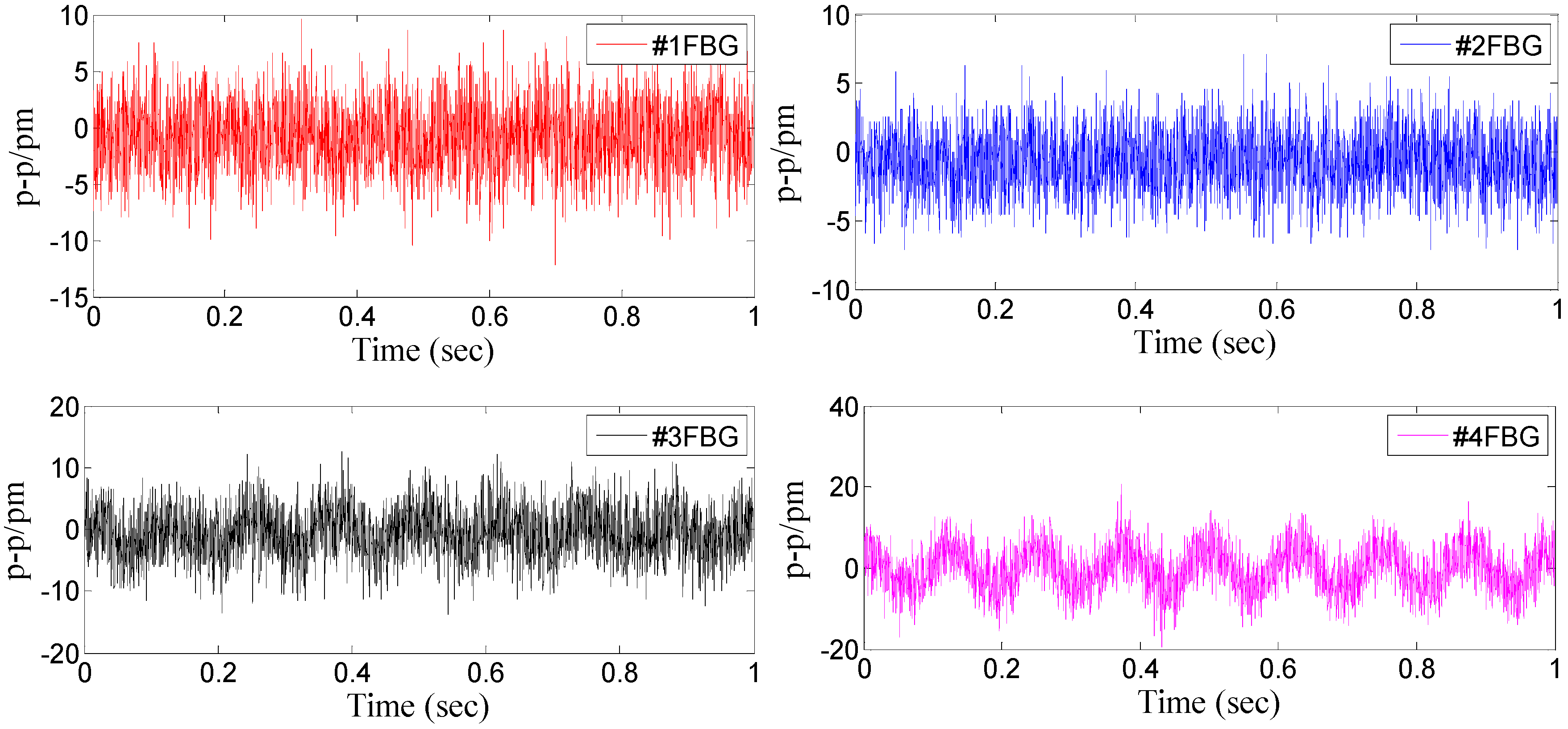
Figure 5 shows a time domain signal of each FBG under the
x-direction excitation with the acceleration—10 m/s
2-200 Hz.
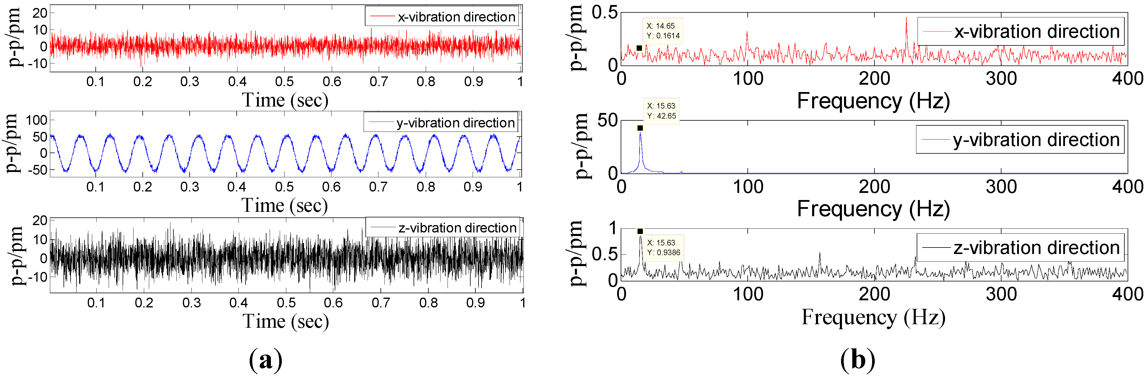
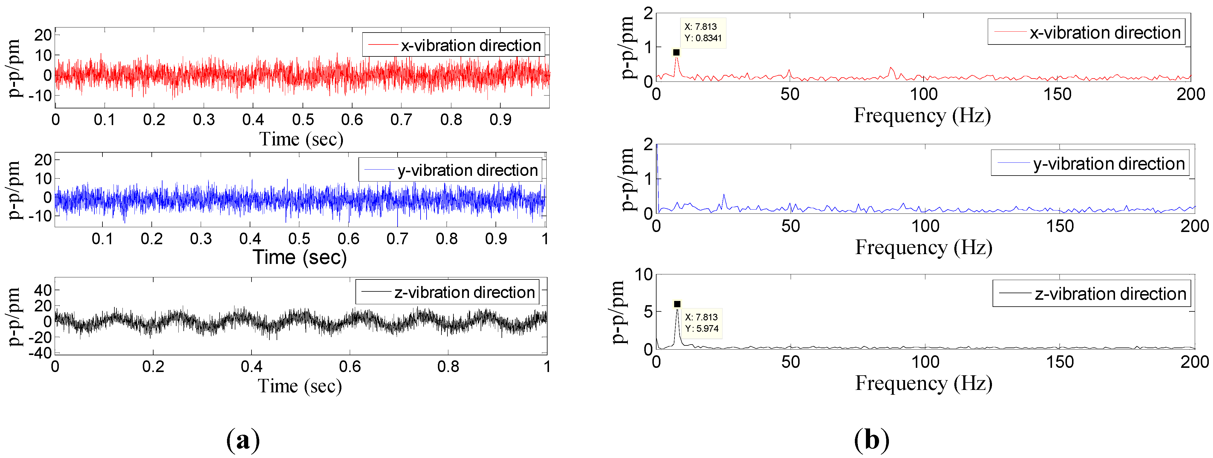
Figure 5 shows that the sine wave response of #1FBG and #2FBG is very clearly compared with the #3FBG and #4FBG, which is consistent with the real situation. Using Equation (15) to dispose the four FBG time domains, the triaxial vibration curves will be attained in
Figure 6. From
Figure 6, we can find that: in the
x-vibration direction, the response is very clear. In addition, there is very little response in the other two directions, which can be ignored compared with response in
x-vibration direction. Thus, the vibration of
x-direction has been discerned by the decoupling principle.
Figure 5.
Time domain signal of each FBG under x-direction excitation with the acceleration—10 m/s2-200 Hz.
Figure 5.
Time domain signal of each FBG under x-direction excitation with the acceleration—10 m/s2-200 Hz.
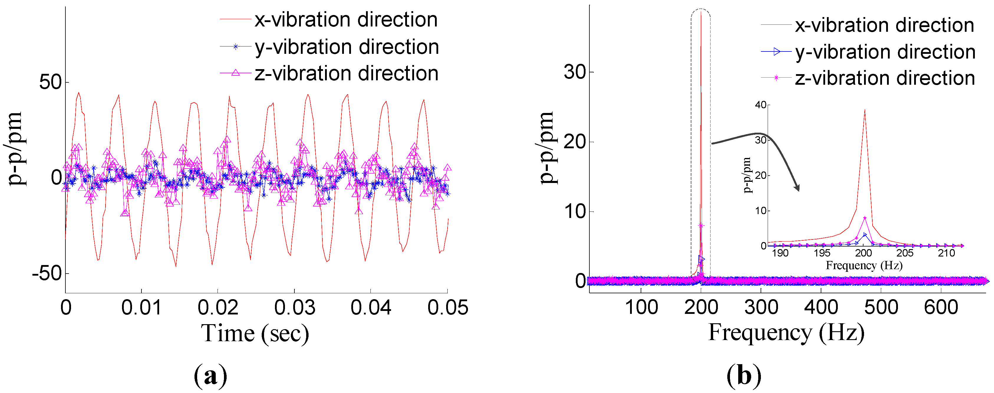
Figure 6.
Response of the three directions under x-direction excitation with the acceleration—10 m/s2-200 Hz. (a) Time domain response map. (b) Spectrum map.
Figure 6.
Response of the three directions under x-direction excitation with the acceleration—10 m/s2-200 Hz. (a) Time domain response map. (b) Spectrum map.
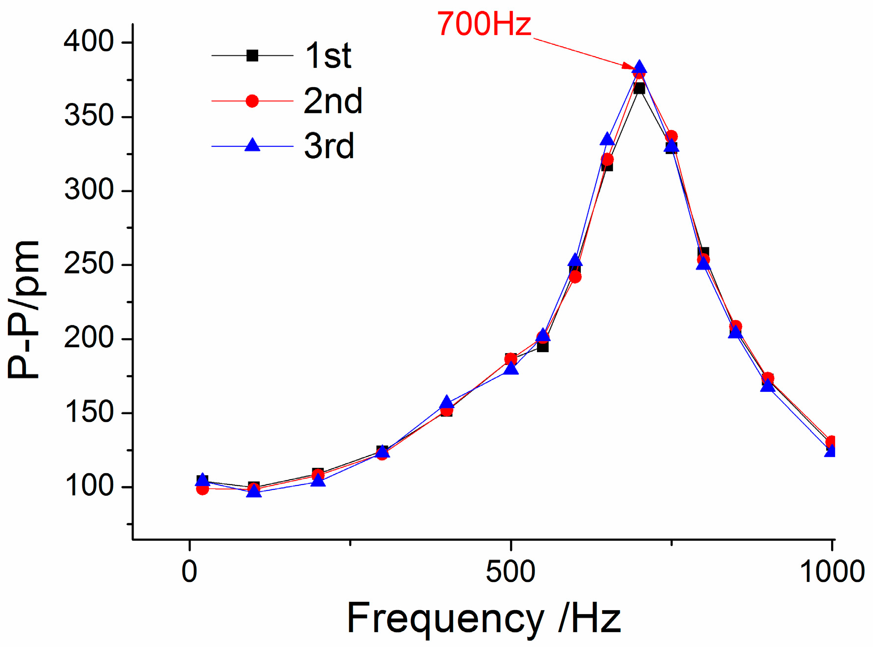
Using a method similar to the above (
Figure 6a) to handle the three experiments’ data, we can get the amplitude-frequency curve of the sensor in the
x-vibration direction (
Figure 7). From
Figure 7, we can get that when frequency is (i) within 20 to 250 Hz, the curve is almost parallel to the horizontal axis in the
x-vibration direction; (ii) equal to 700 Hz, the value of P-P reaches the maximum. Based on the above analysis, for the
x-vibration direction, the working band and the resonant frequency of the sensor are about 10–250 Hz and 700 Hz, respectively.
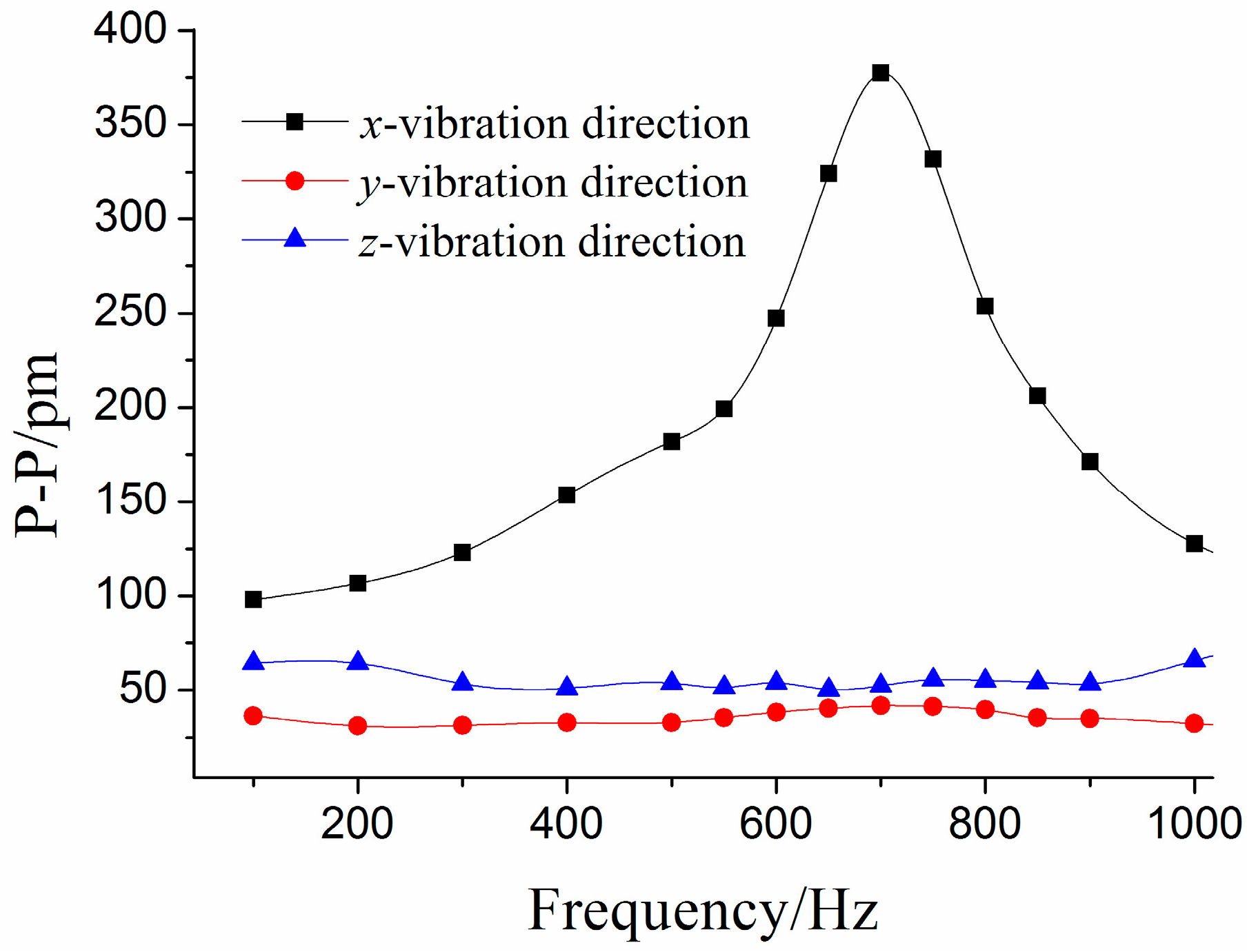
Figure 8 shows the average of center wavelength shifts obtained in the repeated experiments. From
Figure 8, we can get that amplitude-frequency curves of the
y/z direction are almost parallel to horizontal axis, in the
y/z vibration direction the P-P (Peak-peak) values of curve are separately 32.9 pm and 60.6 pm.
Figure 7.
Amplitude-frequency curve of the sensor for the x-vibration direction.
Figure 7.
Amplitude-frequency curve of the sensor for the x-vibration direction.
Figure 8.
Amplitude-frequency curves of each direction under x-direction excitation.
Figure 8.
Amplitude-frequency curves of each direction under x-direction excitation.
With the purpose of investigating the sensor’s properties in the
y-main vibration direction, we change the
y-direction as the main vibration direction. The amplitude of acceleration stays at 1 m/s
2, and frequency of acceleration increases from 3 to 50 Hz.
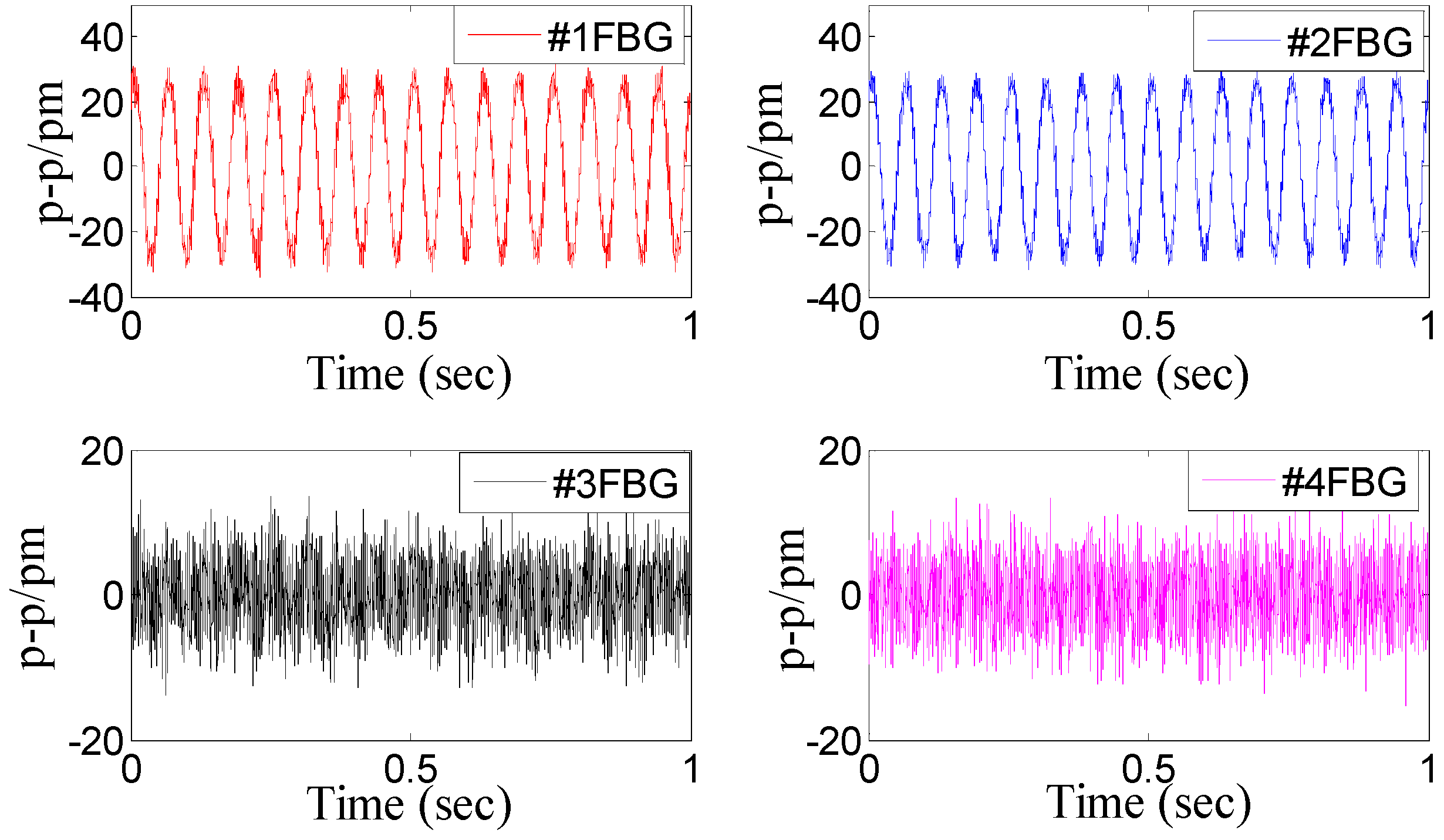
Figure 9 and
Figure 10 are separately showing the response of four FBGs and three direction vibration under
y-vibration excitation. From the two maps, we can find that the response of the
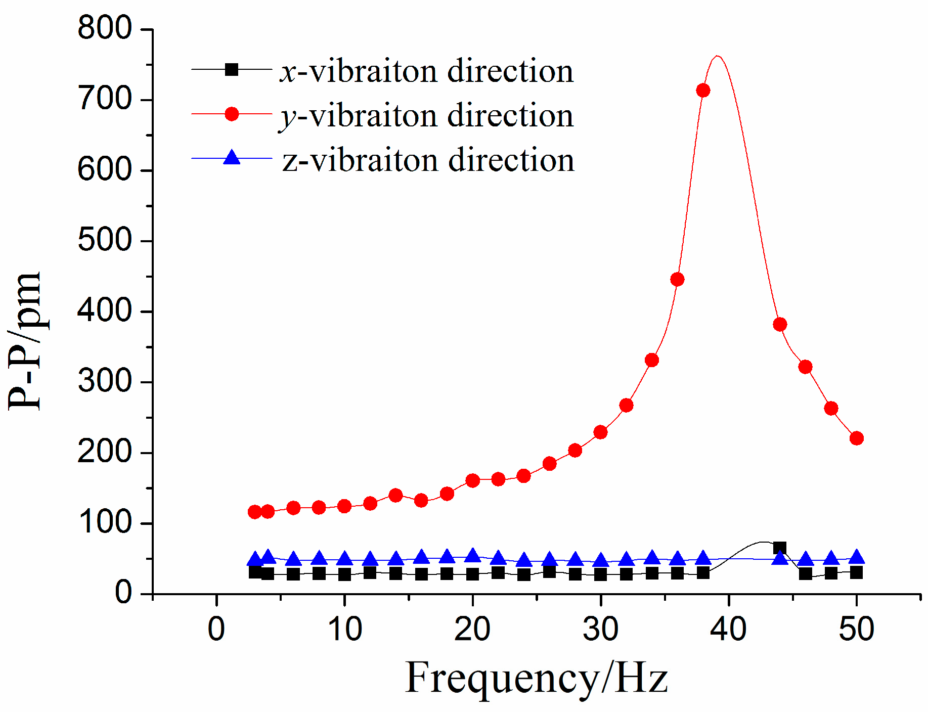
y-direction is more clear than the other two directions. After average value processing for experimental data, amplitude-frequency curves of each direction under
y-direction excitation is shown in
Figure 11. From the
Figure 11, we can get that when frequency is (i) within 3 to 20 Hz, the curve is almost parallel to horizontal axis in the
y-vibration direction; (ii) equal to 40 Hz, the value of P-P reaches the maximum. Therefore, for the
y-vibration direction, the working band and the resonant frequency of the sensor are about 3–20 Hz and 40 Hz, respectively; (iii) the amplitude-frequency curves in the
x/z vibration direction are almost parallel to horizontal axis, in the
x/z direction the P-P values of curve are separately 28.7 pm and 48.5 pm.
Figure 9.
Time domain signal of each FBG under y-direction excitation with the acceleration—1m/s2-16Hz.
Figure 9.
Time domain signal of each FBG under y-direction excitation with the acceleration—1m/s2-16Hz.
Figure 10.
Response of the three directions under y-direction excitation with the acceleration— 1m/s2-16Hz. (a) Time domain response map. (b) Spectrum map.
Figure 10.
Response of the three directions under y-direction excitation with the acceleration— 1m/s2-16Hz. (a) Time domain response map. (b) Spectrum map.
Figure 11.
Amplitude-frequency curves of each direction under y-direction excitation.
Figure 11.
Amplitude-frequency curves of each direction under y-direction excitation.
In order to investigate the sensor’s properties in the
z-main vibration direction, we change the
z-direction as the main vibration direction. The amplitude of acceleration stays at 1 m/s
2, and frequency of acceleration increases from 3 to 120 Hz. The response of four FBGs and three direction vibration under
z-vibration excitation are shown in
Figure 12 and
Figure 13, respectively.
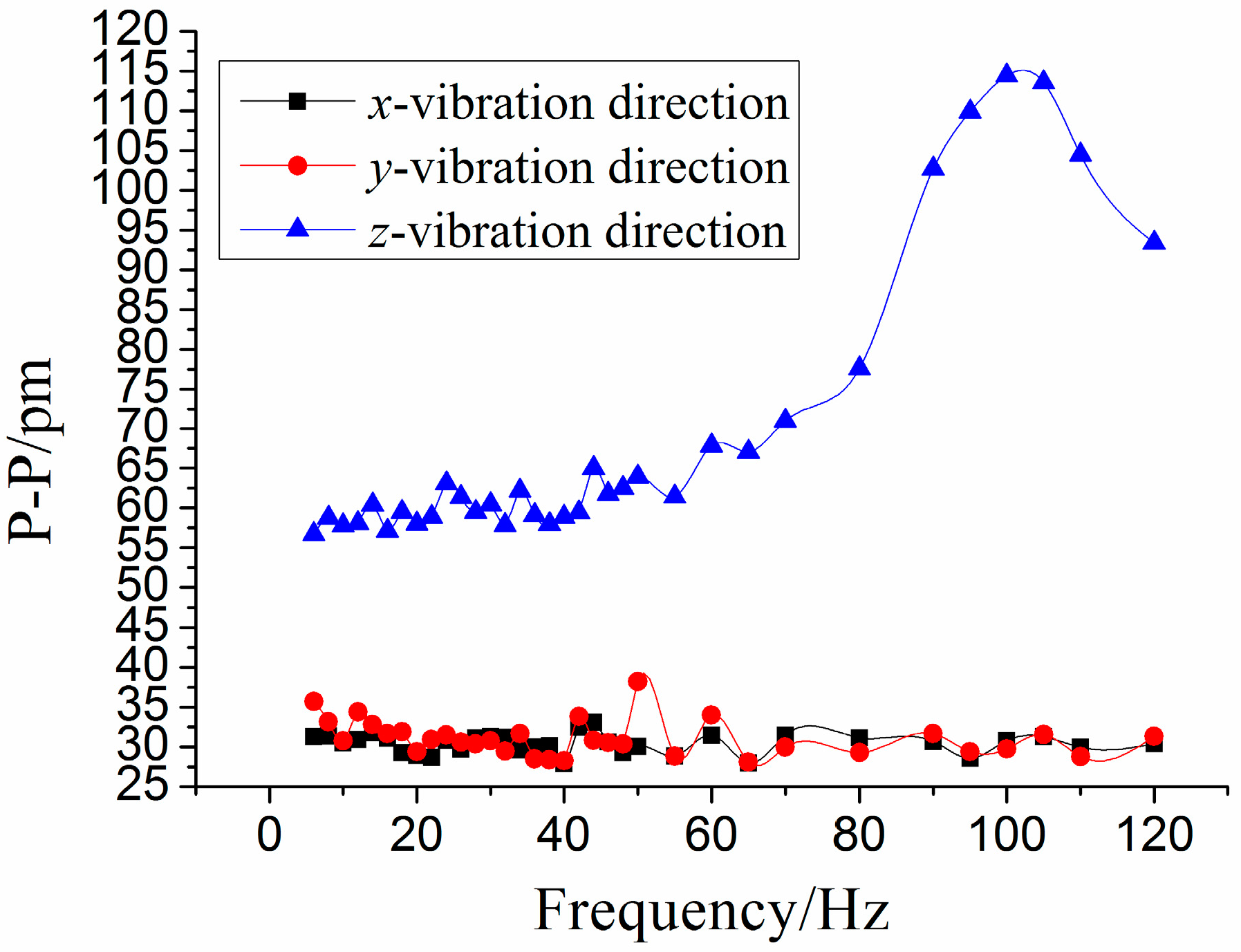
Figure 14 shows the amplitude-frequency curves of each direction under
z-direction excitation. From
Figure 14, we can obtain that when frequency is (i) within 3 to 50 Hz, the curve is almost parallel to horizontal axis for the
z-vibration direction; (ii) equal to 110 Hz, the value of P-P reaches the maximum. Therefore, for the
z-vibration direction, the working band and the resonant frequency of the sensor are about 3–50 Hz and 110 Hz, respectively; (iii) the amplitude-frequency curves in the
x/y vibration direction are almost parallel to horizontal axis, in the
x/y direction, the P-P values of curve are separately 30.5 pm and 31.6 pm.
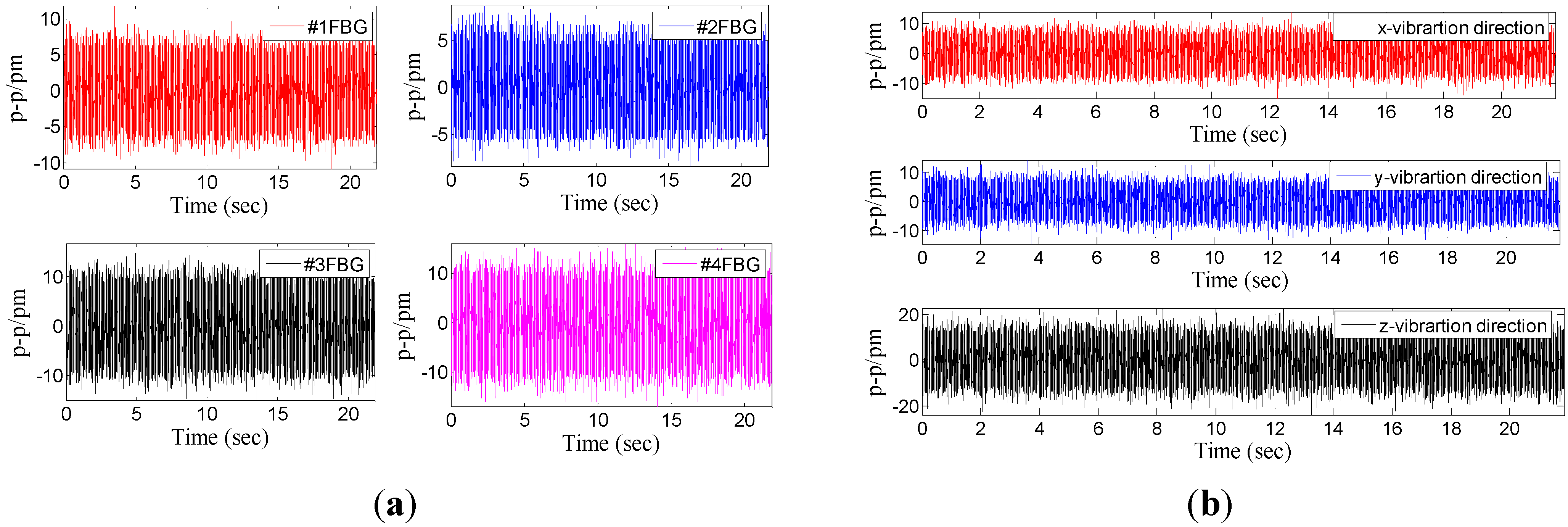
Figure 12.
Time domain signal of each FBG under z-direction excitation with the acceleration—1 m/s2-8 Hz.
Figure 12.
Time domain signal of each FBG under z-direction excitation with the acceleration—1 m/s2-8 Hz.
Figure 13.
Response of the three directions under z-direction excitation with the acceleration—1 m/s2-8 Hz. (a) Time domain response map. (b) Spectrum map.
Figure 13.
Response of the three directions under z-direction excitation with the acceleration—1 m/s2-8 Hz. (a) Time domain response map. (b) Spectrum map.
Figure 14.
Amplitude-frequency curves of each direction under z-direction excitation.
Figure 14.
Amplitude-frequency curves of each direction under z-direction excitation.
3.2. Static Characteristic Experiments of the Sensor
In order to research the static properties of the sensor in the
x-vibration direction, the amplitude of incentive acceleration changes within 5 m/s
2 to 25 m/s
2, and frequency of acceleration is always kept at 100 Hz, which is within the working band 10–200 Hz. In order to demonstrate repeatability of the sensor, the experiment has been repeated four times.
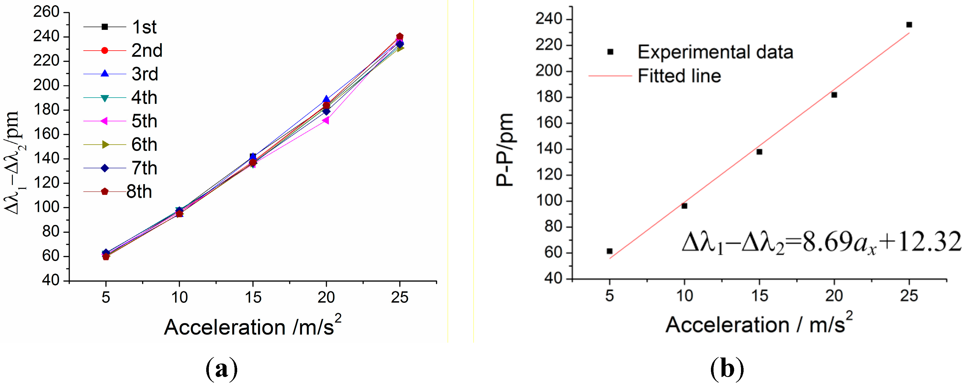
Figure 15 shows difference value Δ
λ1 − Δ
λ2 versus acceleration
ax under
x-direction excitation with the acceleration frequency of 100 Hz. From
Figure 15a, we can get the sensor’s repeatability error is 6.19% and hysteresis error is 9.80%. In
Figure 15b, experimental data is the average of the difference value Δ
λ1 − Δ
λ2 of the repeated experiments. According to the straight line in
Figure 15b, we can obtain the following data: (i) sensitivity of the sensor: 86.9 pm/g; (ii) linearity: 3.64%; (iii) fitted equation: Δ
λ1 − Δ
λ2 = 8.69 ×
ax + 12.32.
Figure 15.
Difference value Δλ1 − Δλ2 versus acceleration ax under x-direction excitation with the acceleration frequency of 100 Hz. (a) Relation between Δλ1 − Δλ2 and acceleration ax within 5–25 m/s2. (b) The linear fitting curve.
Figure 15.
Difference value Δλ1 − Δλ2 versus acceleration ax under x-direction excitation with the acceleration frequency of 100 Hz. (a) Relation between Δλ1 − Δλ2 and acceleration ax within 5–25 m/s2. (b) The linear fitting curve.
For the static properties of sensor in the
y-vibration direction, adjusting the excitation direction along the
y-vibration direction of sensor. In addition, the amplitude of incentive acceleration changes within 1 m/s
2 to 4.5 m/s
2, and frequency of acceleration is always kept at 8 Hz, which is within the working band 3–20 Hz. The experiment is repeated four times.
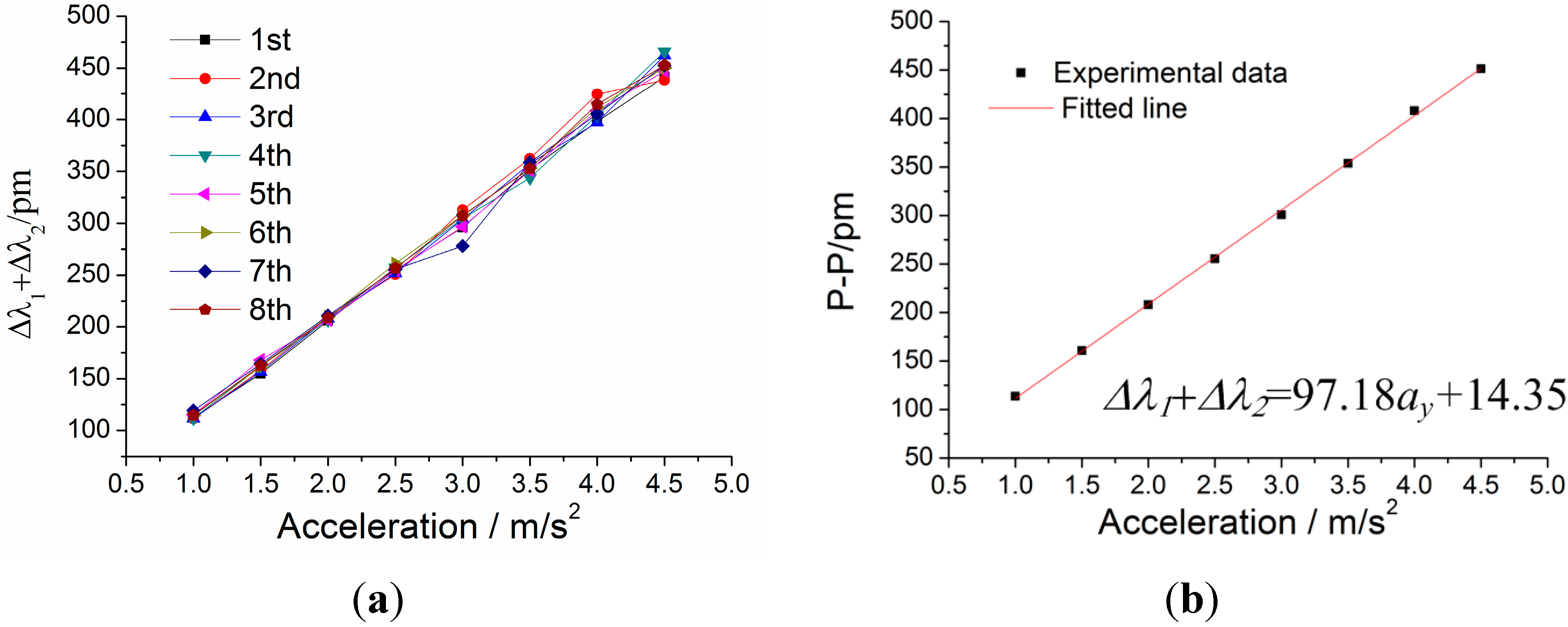
Figure 16 shows addition value Δ
λ1 + Δ
λ2 versus acceleration
ay under
y-direction excitation with the acceleration frequency of 100 Hz. From
Figure 16a, we can get that the sensor’s repeatability error is 8.65% and hysteresis error is 8.15%. In
Figure 16b, experimental data is the average of the difference value Δ
λ1Δ
λ2 in the repeated experiments. According to the straight line in
Figure 16b, we can obtain the following data: (i) sensitivity of the sensor: 971.8 pm/g; (ii) linearity: 1.50%; (iii) fitted equation: Δ
λ1 + Δ
λ2 = 97.18 ×
ay + 14.35.
Figure 16.
Addition value Δλ1 + Δλ2 versus acceleration ay under y-direction excitation with the acceleration frequency of 8 Hz. (a) Relation between Δλ1 + Δλ2 and acceleration ay within 1–4.5 m/s2. (b) The linear fitting curve.
Figure 16.
Addition value Δλ1 + Δλ2 versus acceleration ay under y-direction excitation with the acceleration frequency of 8 Hz. (a) Relation between Δλ1 + Δλ2 and acceleration ay within 1–4.5 m/s2. (b) The linear fitting curve.
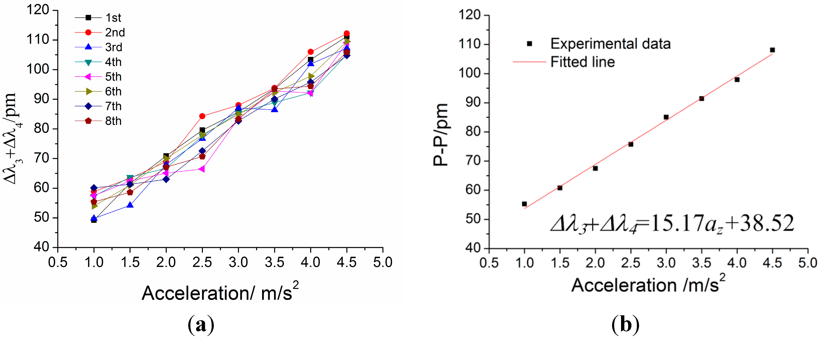
For the static properties of sensor in the
z-vibration direction, the amplitude of incentive acceleration changes within 1 m/s
2 to 4.5 m/s
2, and frequency of acceleration is always kept at 8 Hz, which is within the working band 3–50 Hz. The experiment is repeated four times.
Figure 17 shows addition value Δ
λ3 + Δ
λ4 versus acceleration
az under
z-direction excitation with the acceleration frequency of 100 Hz. According to the straight line in
Figure 17b, we can obtain the following data: (i) sensitivity of the sensor: 151.7 pm/g; (ii) linearity: 3.01%; (iii) fitted equation: Δ
λ3 + Δ
λ4 = 15.17 ×
az + 38.52.
Figure 17.
Addition value Δλ3 + Δλ4 versus acceleration az under z-direction excitation with the acceleration frequency of 8 Hz. (a) Relation between Δλ3 + Δλ4 and acceleration az within 1–4.5 m/s2. (b) The linear fitting curve.
Figure 17.
Addition value Δλ3 + Δλ4 versus acceleration az under z-direction excitation with the acceleration frequency of 8 Hz. (a) Relation between Δλ3 + Δλ4 and acceleration az within 1–4.5 m/s2. (b) The linear fitting curve.


