
Shaft Diameter Measurement Using Structured Light Vision

College of Mechanical Science and Engineering, Jilin University, Changchun 130022, China
*
Author to whom correspondence should be addressed.
Sensors 2015, 15(8), 19750-19767; https://doi.org/10.3390/s150819750
Submission received: 9 April 2015
/
Revised: 1 August 2015
/
Accepted: 6 August 2015
/
Published: 12 August 2015
(This article belongs to the Section Physical Sensors)
Abstract
:A method for measuring shaft diameters is presented using structured light vision measurement. After calibrating a model of the structured light measurement, a virtual plane is established perpendicular to the measured shaft axis and the image of the light stripe on the shaft is projected to the virtual plane. On the virtual plane, the center of the measured shaft is determined by fitting the projected image under the geometrical constraints of the light stripe, and the shaft diameter is measured by the determined center and the projected image. Experiments evaluated the measuring accuracy of the method and the effects of some factors on the measurement are analyzed.
1. Introduction
Shafts are one of most important machine elements and the accuracy of machined shafts has a significant effect on the properties of any mechanical device that employs one. The accuracy of a machined shaft can be ensured using a Computer Numerical Control lathe, but mechanical wear in a CNC lathe system, system deformation, and the radial wear of the machining tools will reduce the accuracy of the machined shaft. If the variation of the shaft diameter could be monitored during its machining, the dimensional accuracy of the product could be ensured by the automatic compensation system of the CNC lathe. Therefore, on-line measurement of shaft size is very important in machining.
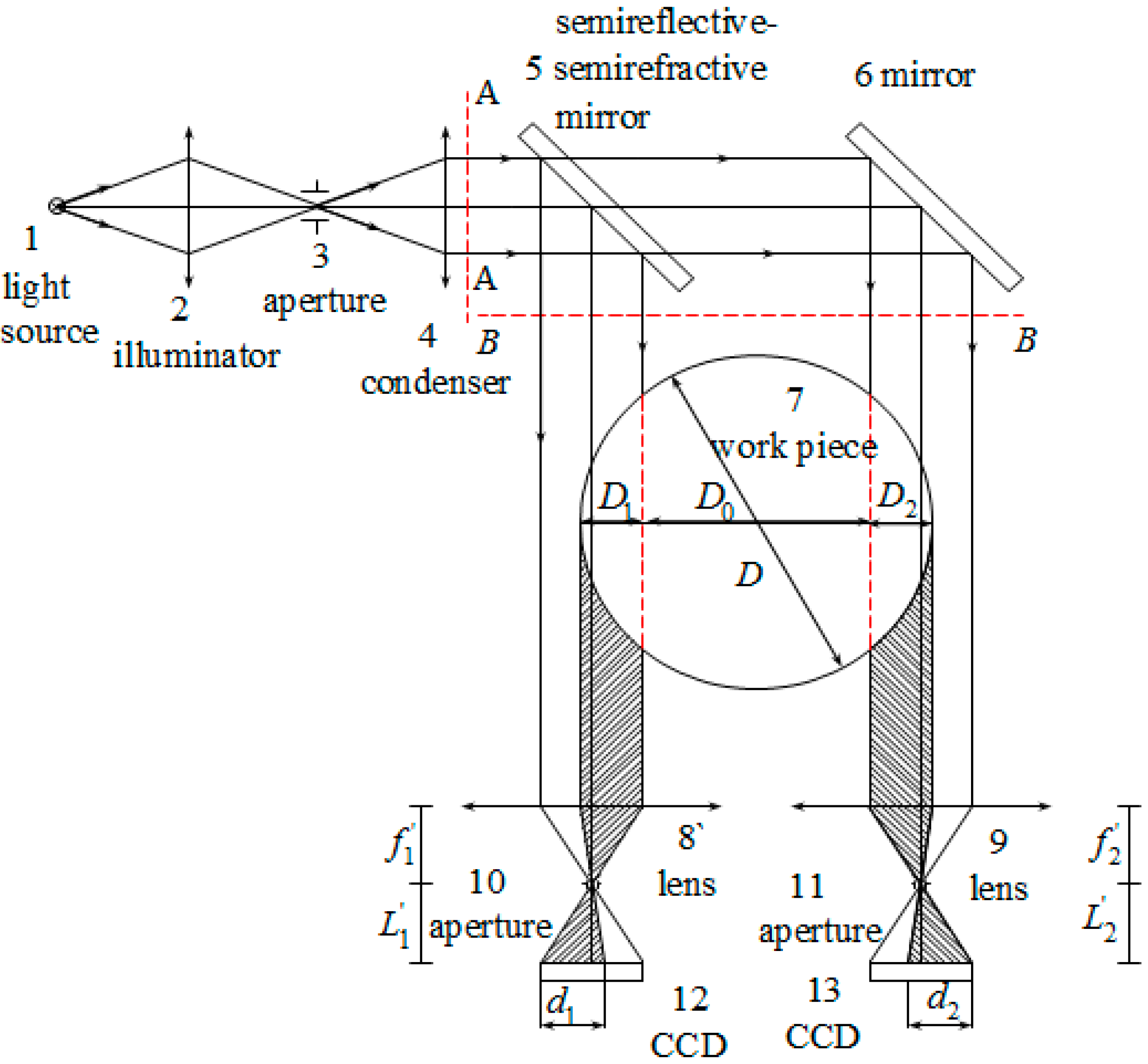
A variety of noncontact machine vision methods for measuring the product diameters have been proposed [1,2,3,4,5]. These methods can be classified as active methods and passive methods. Passive measurement methods use a camera or two cameras to obtain shaft diameters [6,7]. In 2008, Song et al. [8] proposed a method where both edges of a shaft were imaged onto two cameras through two parallel light paths as shown in Figure 1 [8]. Using this approach, the shaft diameter was obtained by measuring the length of the photosensitive units on the shadow field of the two CCDs (Charge-Coupled Device) and the distance between the two parallel light paths. This method can amplify the measurement range while ensuring the measuring accuracy; however, it is very difficult to calibrate the position of the two cameras.
Figure 1.
The optical principle of the parallel light projection method with double light paths (with permission from [8]).
Figure 1.
The optical principle of the parallel light projection method with double light paths (with permission from [8]).

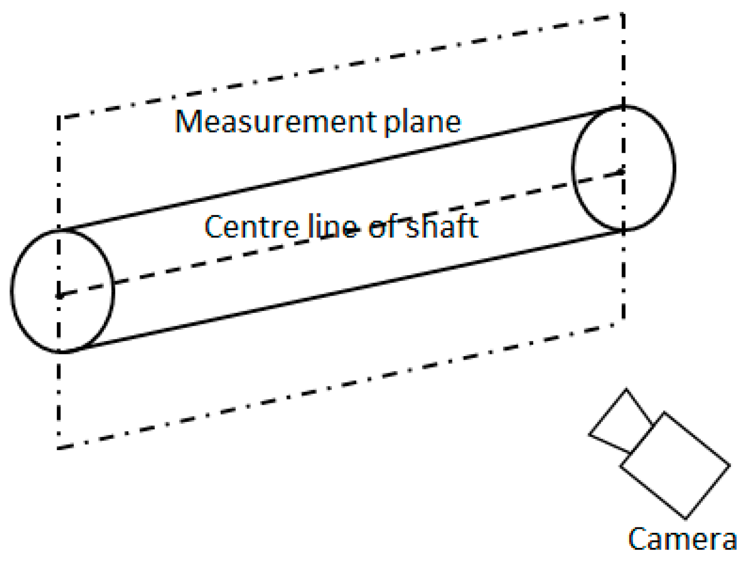
In 2013, Sun [9] used a camera to obtain shaft diameters, employing a theory of plane geometry in the cross-section, which is perpendicular to the axis of the shaft, as shown in Figure 2 [9]. This method can achieve a high measuring accuracy, but it requires the calibration of the plane of the center line of the shaft before the measurement. In practice, the position of the center line changes each time the shaft is clamped by the jaw chucks of the lathe. This change of position will decrease the accuracy of measurement.
Figure 2.
The orientations of the shaft and the measurement plane in 3D space (with permission from [9]).
Figure 2.
The orientations of the shaft and the measurement plane in 3D space (with permission from [9]).
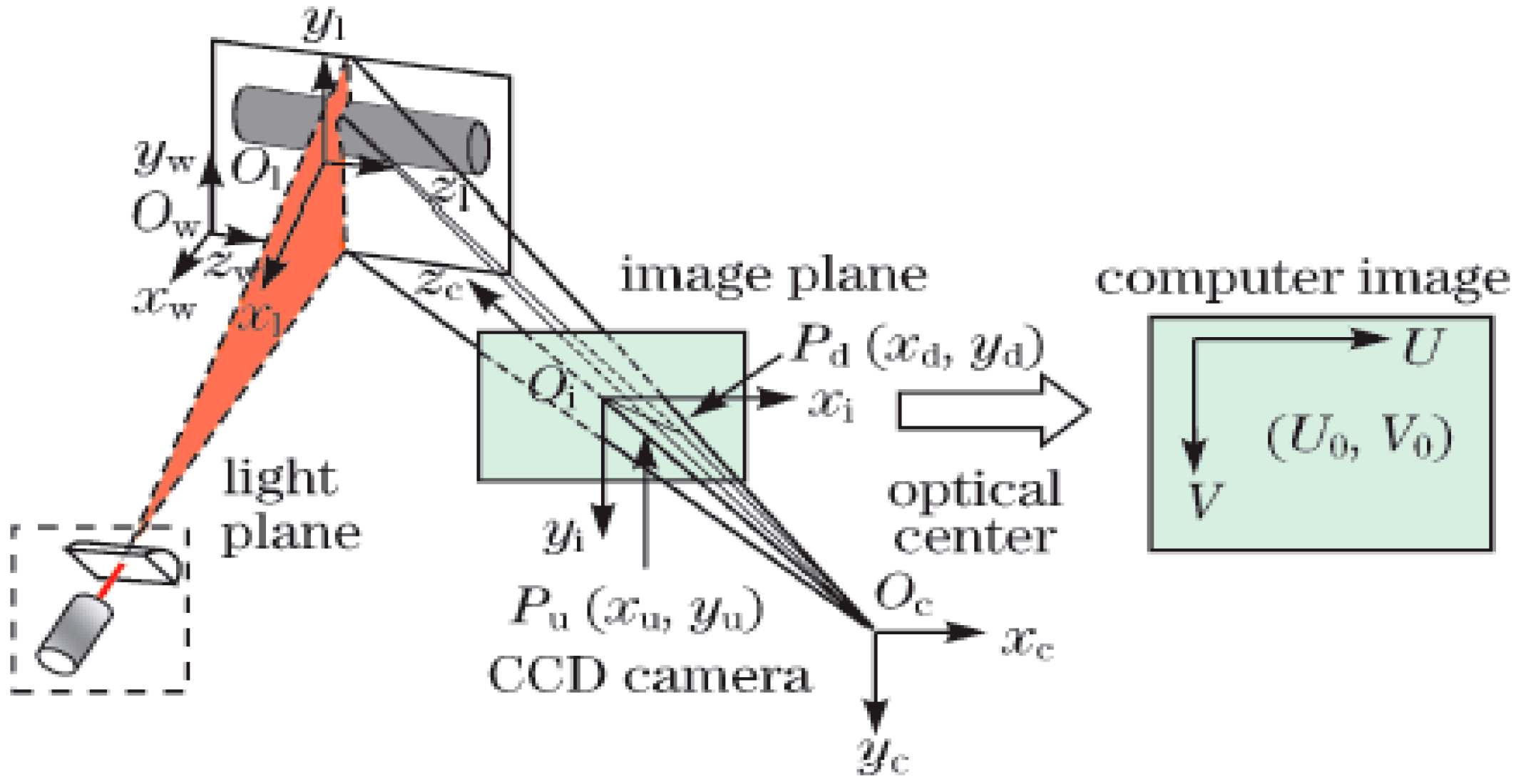
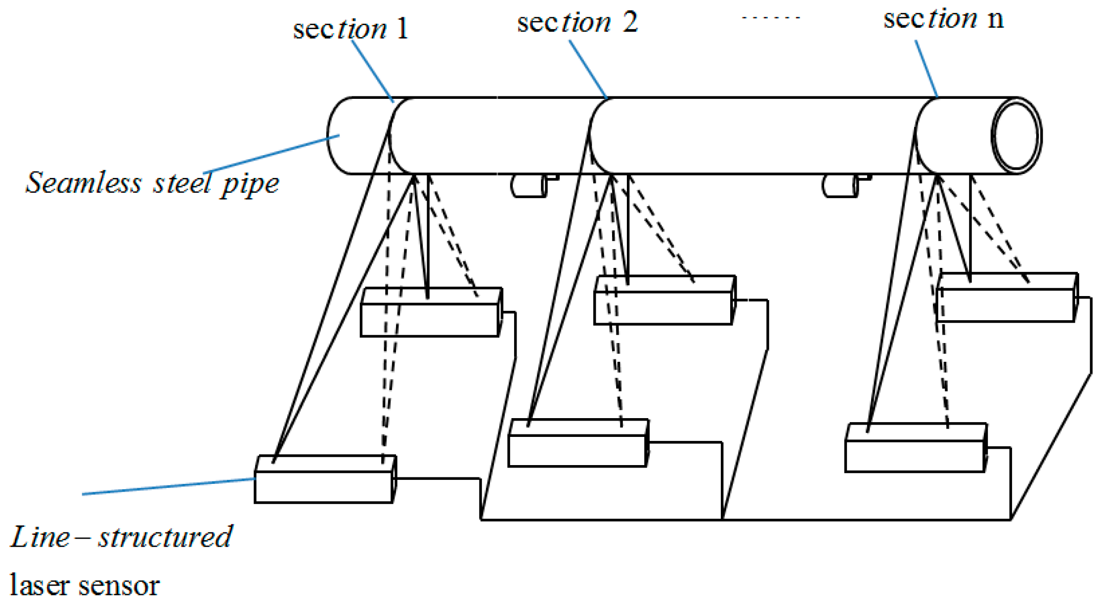
Active measurement methods generally use one or more cameras and lasers to achieve accurate measurements of shaft diameters. In 2001, Sun et al. [10] used a pair of line-structured lasers and cameras to measure shaft diameters, as shown in Figure 3 [10]. The lights was projected onto the pipe, then captured by two cameras, and the diameter of a steel pipe could be determined by fitting the ellipse with the two developed arcs. It is difficult to ensure that the two arcs are on the same plane, so the accuracy of the method is limited. In 2010, Liu et al. [11] reported a method for measuring shaft diameters using a line-structured laser and a camera, as shown in Figure 4 [11]. The coordinates of the light stripe projected on the shaft were obtained using a novel gray scale barycenter extraction algorithm along the radial direction. The shaft diameter was then obtained by circle fitting using the generated coordinates. If the line-structured light is perpendicular to the measured shaft, the shaft diameter can be obtained by fitting a circle. Thus, this method is limited by the measurement environment.
Figure 3.
Sketch of the measurement system (with permission from [10]).
Figure 3.
Sketch of the measurement system (with permission from [10]).

Figure 4.
Mathematical model of the system (with permission from [11]).
Figure 4.
Mathematical model of the system (with permission from [11]).
In this study, a method for measuring shaft diameter is proposed using a line-structured laser and a camera. Based on the direction vector of the measured shaft axis, which is calibrated before the measurement, a virtual plane is established perpendicular to the axis and the image of a light stripe on the shaft is projected to the virtual plane. The shaft diameter is then determined from the projected image on the virtual plane. To improve the measuring precision, the center of the projected image was determined by fitting the projected image using a set of geometrical constraints.
2. Calibration of the Structure Light Measuring System
2.1. Calibration of Camera Parameters
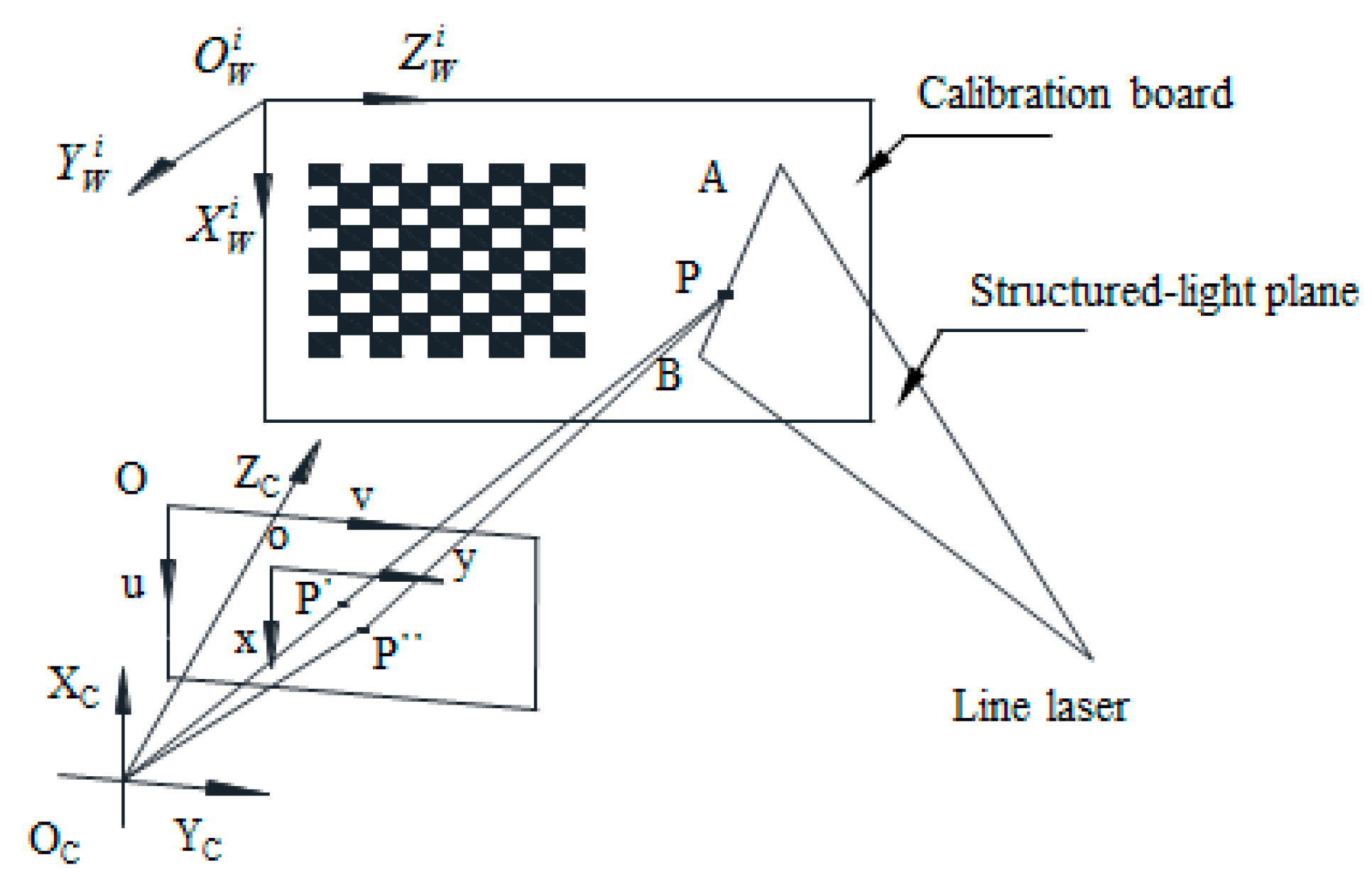
The calibration of the measurement system employed world coordinate systems (OiWXiWYiWZiW), a camera coordinate system (OCXCYCZC), a image coordinate system (oxy), and a pixel coordinate system (Ouv), which were established as shown in Figure 5.
Figure 5.
Calibration model of the line structured light.
Based on pinhole projection and lens distortion models, the mapping from the world coordinates to the pixel coordinates can be expressed as reported by Zhang [12] and shown in Table 1, where R is the rotation matrix; T is translation vector; k1, k2, p1, and p2 are the coefficients of radial and tangential distortions; is the interior camera parameters; ZW = 0 in the model. A nonlinear function can be established by minimizing the distance between the calculated pixel coordinates of the corner points in the calibration board and the actual pixel coordinates. The function was solved using the Levenberg-Marquardt algorithm [13].

| Transformation | Equations | |
|---|---|---|
| From world coordinates to camera coordinates | (1) | |
| From camera coordinates to image coordinates | (2) | |
| Introduce the distortion model, where, r2=x2d+y2d, | (3) | |
| From image coordinates to pixel coordinates | (4) | |
2.2. Calibration of Structured Light Parameters
The calibration model of the structured light is shown in Figure 5. Here, AB is the intersection line between the light plane and the calibration board, P is a point on AB. The pixel coordinate of P can be extracted as described by Steger [14], and camera coordinates of P are determined using Equations (1)–(4). Different intersection lines can be obtained by turning the board, so Pij is the jth point on the intersection line when the board is in the ith position.
Setting the equation of the light plane under OCXCYCZC:
The parameters b1, b2, b3 can be determined by the objective function:
where n is number of board turns, k is the number of sample points on the intersection line when the board is in the ith position, and (XiCj,YiCj, ZiCj) are camera coordinates of Pij. According to the principle of least squares, the coefficients of Equation (5) can be solved as:
Because the camera parameters and coordinates of the sample points have errors, the coefficients obtained by Equation (7) will be used as initial values for optimizing the light plane. The objective function of the optimized plane is established by the distances between the points and the plane:
The parameters of the plane can be obtained using the Levenberg-Marquardt algorithm. In the experiment, when the constant term of Equation (5) is 1, the parameters of the plane are small and the denominator of Equation (8) is around 0. To improve the optimization results, the constant term of Equation (5) is set at 1000 in the paper.
3. The Principle and Model of the Measurement
The model for measuring the shaft diameters is shown in Figure 6. A shaft is clamped at two centers, images of the shaft are captured by a CCD camera, п1 is the light plane, and MN is the axis of the shaft. The stripe ab is formed by projecting the light plane п1 onto the measured shaft. The pixel coordinates of ab stripe centers are extracted by Steger’s algorithm. The virtual plane п2 perpendicular to the measured shaft is created and the normal vector of п2 is the directional vector of the axis MN. Although the position of the axis changes slightly every time a shaft is clamped, the direction of the axis does not change. Thus, the equation of the virtual plane п2 can be obtained in OCXCYCZC (see Appendix A for the details):
The arc cd is formed by the virtual plane п2 intersecting the measured shaft.
Figure 6.
The measurement model of the shaft. (a) global view, (b) local view.

Since the light plane п1 is not perpendicular to the shaft, the cross-section is an ellipse and the shaft diameter can be obtained by fitting the ellipse with stripe centers Pi. The elliptic equation is:
The parameters of Equation (10) can be obtained by the least squares method, and the length of the minor axis d is the measured shaft diameter:
Since the virtual plane п2 is perpendicular to the shaft, the cross-section is a circle and the diameter can be obtained by fitting the circle with points Qi, which are Pi projecting on the virtual plane п2. The circle equation is
The parameters of Equation (12) can be obtained by the least squares method, and the circle diameter d1 is the measured shaft diameter:
Since the pixel coordinates of the extracted stripe centers have errors, from the numerical analysis, the measuring accuracy of the shaft diameter by circle fitting is better than by ellipse fitting (see Appendix B for the detail).
The image coordinates of Pi can be achieved using Equations (3) and (4), so the equations of OCPi are:
The camera coordinates can be obtained using Equations (5) and (14):
A set of lines PiQi are made by passing through the extracted centers and parallel to the measured shaft axis, as shown in Figure 6b. Since the axis MN is perpendicular to the plane п2, the direction vectors of the lines are the normal vector of п2, . Thus, the equations of lines PiQi are:
Each line PiQi has an intersection point Qi on the plane п2. The camera coordinates of the intersection points are obtained using Equations (9) and (16), respectively.
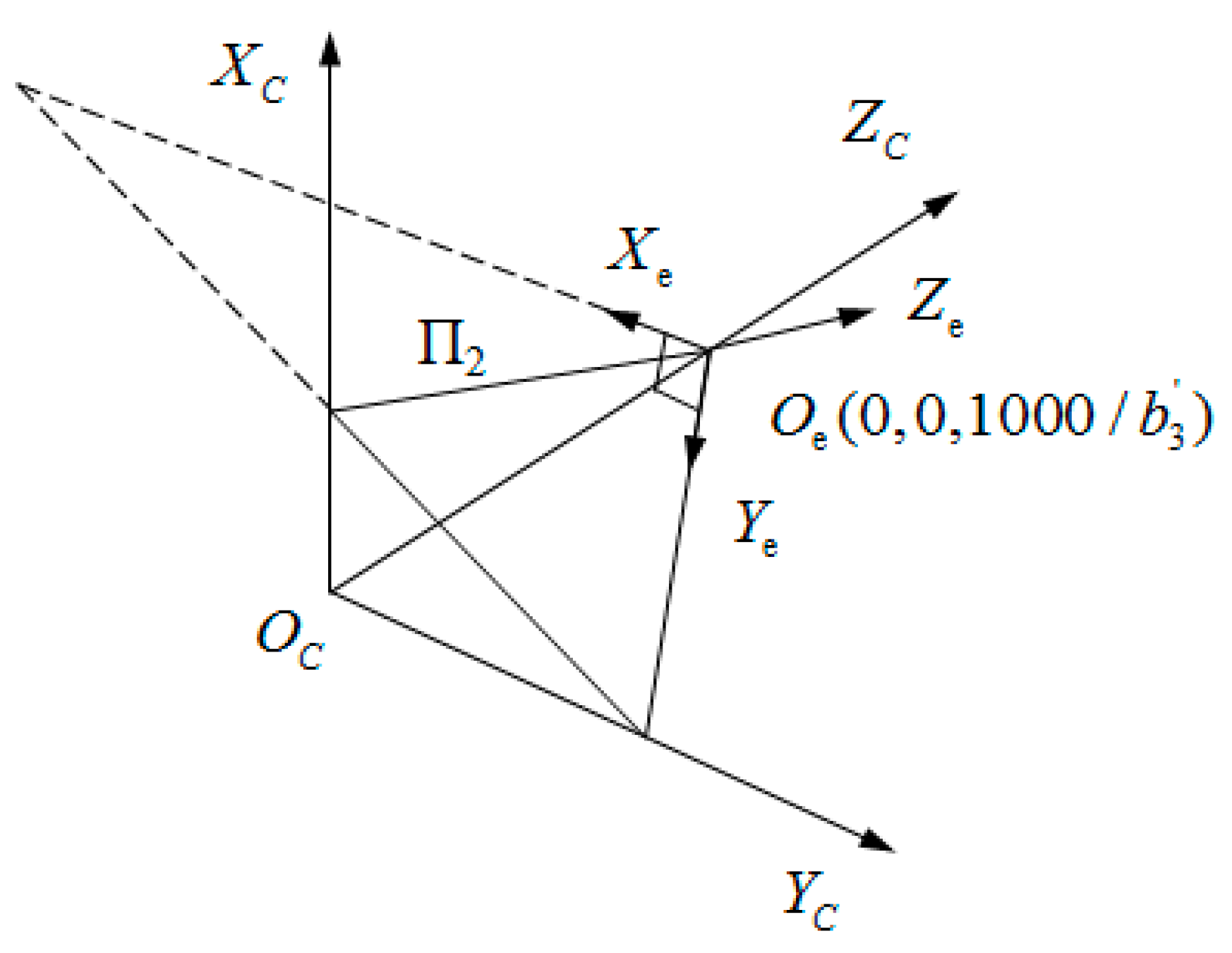
Figure 7.
Oe—XeYeZe and OC—XCYCZC.

To facilitate the circle fitting, a coordinate system (Oe—XeYeZe) is established on the plane п2, as shown in Figure 7. In Oe—XeYeZe, XeYe plane is the plane п2, OeZe axis is perpendicular to the plane п2, and the origin of coordinate Oe is the intersection point of the plane п2 with OCZC axis. Additionally, camera coordinates of the origin of Oe can be obtained by Equation (9). Thus, translations of the camera coordinate system are relative to Oe—XeYeZe and the camera coordinate Qi can be changed into Oe—XeYeZe by Equation (17):
where, is the rotation angle round OCYC, is the rotation angle round OCXC, and are the coordinates of in Oe—XeYeZe.
Normal vector of the plane п2 is converted by the coordinate rotation into in Oe-XeYeZe, where, . Thus, values before and after the conversion are substituted into Equation (18):
and are obtained by Equation (18). In Oe-XeYeZe, because points Qi are on п2, the coordinates Qi are .
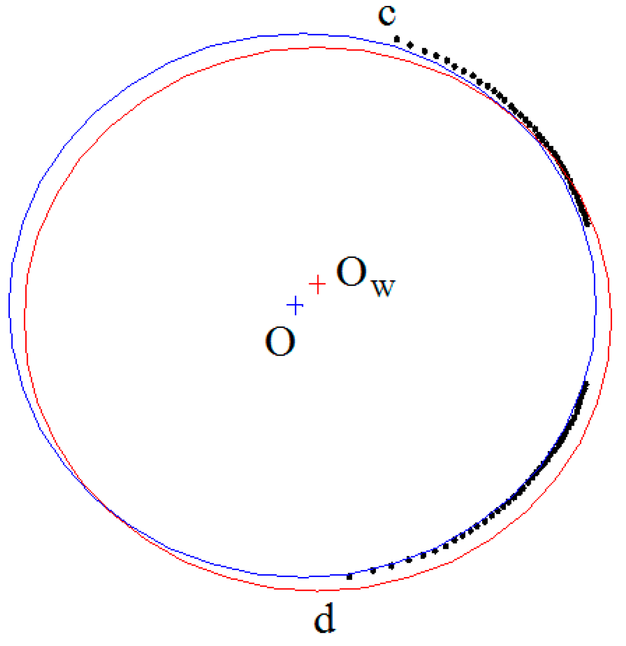
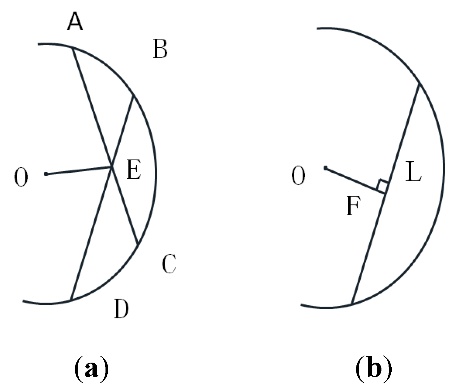
Since arc cd is at a side of the shaft and the coordinates of points Qi on cd have errors, the accuracy of the shaft diameter which is directly measured by fitting points on cd is poor, as shown in Figure 8. In Figure 8, the red circle is a cross-section formed by the virtual plane п2 intersecting with the shaft and Ow is the center of the red circle. The circle obtained by fitting the black points on cd is blue with its center at O. To improve the measuring accuracy, the center is determined by fitting black points under the geometrical constraints of arc cd, and the geometrical constraints for a circle center are shown in Figure 9.
In Figure 9a, A, B, C, D are the fitting points in the circle and O is the center. Point E is the intersection point of AC and BD. From the geometrical feature of a circle, the following relation holds:
where r is radius of the shaft. Setting the center coordinate as (x0,y0), the coordinates of the points A, B, C, D are (xa,ya), (xb,yb), (xc,yc), (xd,yd). The coordinate (xe,ye) of point E can be obtained from points A, B, C, D. Thus, the first objective function can be presented as:
where the value of r is estimated when optimizing Equation (20); n is number of the points.
Figure 8.
Fitting circle by limited data.

Figure 9.
Geometrical features of a circle. (a) constraint condition1; (b) constraint condition2.

As shown in Figure 9b, F is the midpoint of the chord L. Thus, line OF is perpendicular to the chord L and can be presented as:
Therefore, the center coordinate can be determined by Equations (20) and (21):
Minimizing Equation (22) is a nonlinear minimization problem, which can be solved by the Levenberg-Marquardt algorithm. The initial value of the center is obtained by fitting the circle with the points in cd.
Finally, the shaft diameter is obtained by the distance between the points in cd and the optimized center:
where d is the diameter of shaft, (xi,yi) are coordinates of the points in cd, (X0,Y0) is the coordinate of the optimized center, and n is the number of fitting points.
4. Experiments and Analysis
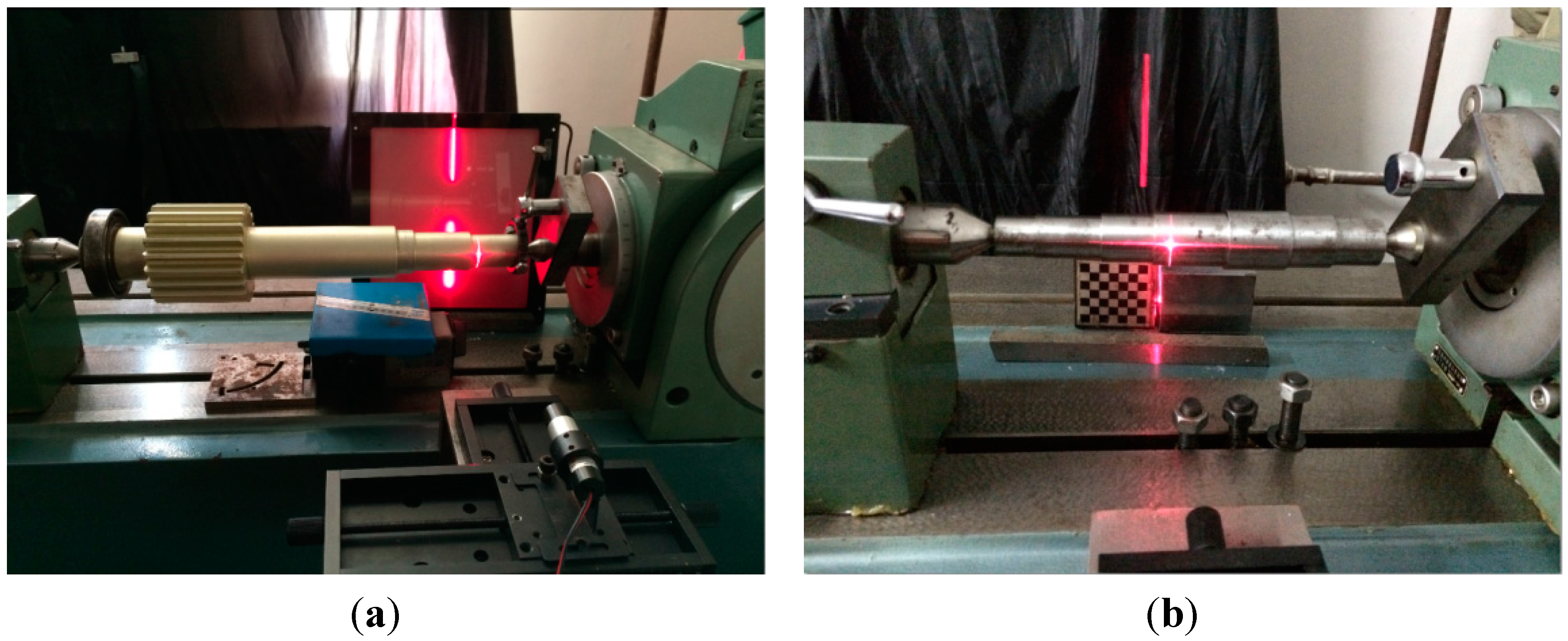
Experiments were conducted to assess the utility of the proposed method. The experimental equipment employed is shown in Figure 10 and the main parameters of the equipment are shown in Table 2. The interior parameters of the camera were calibrated by the method presented in Section 2. Two shafts were used in the experiments; shaft 1 was a four-segment shaft and the shaft surface’s reflection was reduced using a special process, as shown in Figure 10a. Shaft 2 was a seven-segment shaft, as shown in Figure 10b. The shafts’ diameters were measured using a micrometer with a resolution of 1 μm.
Figure 10.
Experimental equipment for measuring shafts: (a) shaft 1; (b) shaft 2.

| Equipment | Mold NO. | Main Parameters |
|---|---|---|
| CCD camera | JAI CCD camera | Resolution: 1376 × 1024 |
| Lens | M0814-MP | Focal length: 25 mm |
| Line projector | LH650-80-3 | Wavelength: 650 nm |
| Mold plane CBC75mm-2.0 | Precision of the grid: 1 μm | |
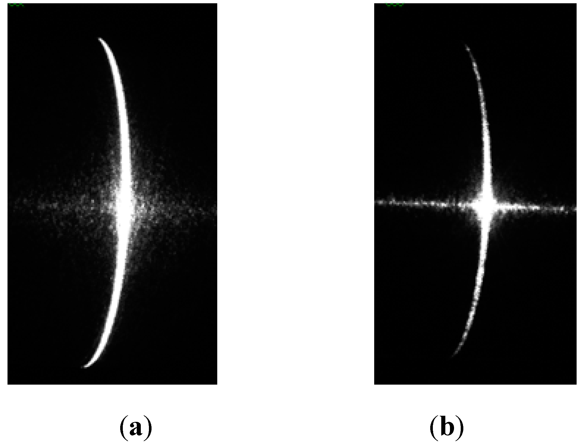
First, the images of the shafts were captured using the camera, as shown in Figure 11. The diameters of the shafts were measured using the method described in Section 3. The measurement data are listed in Table 3 and Table 4, and the measurement error was less than 25 μm.
Figure 11.
Images of stripes by camera: (a) shaft 1; (b) shaft 2.

| NO. | 1 | 2 | 3 | 4 |
|---|---|---|---|---|
| Measurement results | 47.05 | 39.749 | 34.915 | 29.796 |
| Known values | 47.062 | 39.76 | 34.924 | 29.8 |
| Errors | 0.012 | 0.011 | 0.009 | 0.004 |
| NO. | 1 | 2 | 3 | 4 | 5 | 6 | 7 |
|---|---|---|---|---|---|---|---|
| Measurement results | 24.761 | 27.661 | 31.456 | 27.474 | 24.596 | 21.696 | 20.091 |
| Known values | 24.753 | 27.664 | 31.473 | 27.492 | 24.621 | 21.687 | 20.113 |
| Errors | 0.008 | 0.003 | 0.017 | 0.018 | 0.025 | 0.009 | 0.022 |
To compare the proposed method with the other methods, the diameters of the shafts were obtained by directly fitting the ellipse and circle. The data for these methods are shown in Table 5 and Table 6. The measuring accuracy of the present method was found to be better than that of the other two methods.
| NO. | D | Fitting Ellipse | Fitting Circle | Present Method | |||
|---|---|---|---|---|---|---|---|
| D1 | Errors | D2 | Errors | D3 | Errors | ||
| 1 | 47.062 | 46.992 | 0.07 | 47.034 | 0.028 | 47.05 | 0.012 |
| 2 | 39.76 | 39.659 | 0.101 | 39.698 | 0.062 | 39.749 | 0.011 |
| 3 | 34.924 | 34.773 | 0.151 | 34.827 | 0.097 | 34.915 | 0.009 |
| 4 | 29.8 | 29.741 | 0.059 | 29.73 | 0.07 | 29.796 | 0.004 |
| Mean error | 0.095 | 0.064 | 0.009 | ||||
To test the influence of the angle between the light plane and cross-section of the shaft on the proposed method, the shaft diameters were measured by light planes with three different light angles, as shown in Figure 12. Measurement results are listed in Table 7 and Table 8.
| NO. | D | Fitting Ellipse | Fitting Circle | Present Method | |||
|---|---|---|---|---|---|---|---|
| D1 | Errors | D2 | Errors | D3 | Errors | ||
| 1 | 24.753 | 24.203 | 0.55 | 24.62 | 0.133 | 24.761 | 0.008 |
| 2 | 27.664 | 27.193 | 0.471 | 27.632 | 0.032 | 27.661 | 0.003 |
| 3 | 31.473 | 30.877 | 0.596 | 31.395 | 0.078 | 31.456 | 0.017 |
| 4 | 27.492 | 27.098 | 0.394 | 27.415 | 0.077 | 27.474 | 0.018 |
| 5 | 24.621 | 24.097 | 0.524 | 24.512 | 0.109 | 24.596 | 0.025 |
| 6 | 21.687 | 21.224 | 0.463 | 21.624 | 0.063 | 21.696 | 0.009 |
| 7 | 20.113 | 19.705 | 0.408 | 19.935 | 0.178 | 20.091 | 0.022 |
| Mean error | 0.487 | 0.096 | 0.015 | ||||
Figure 12.
Images of stripes at three different angles.
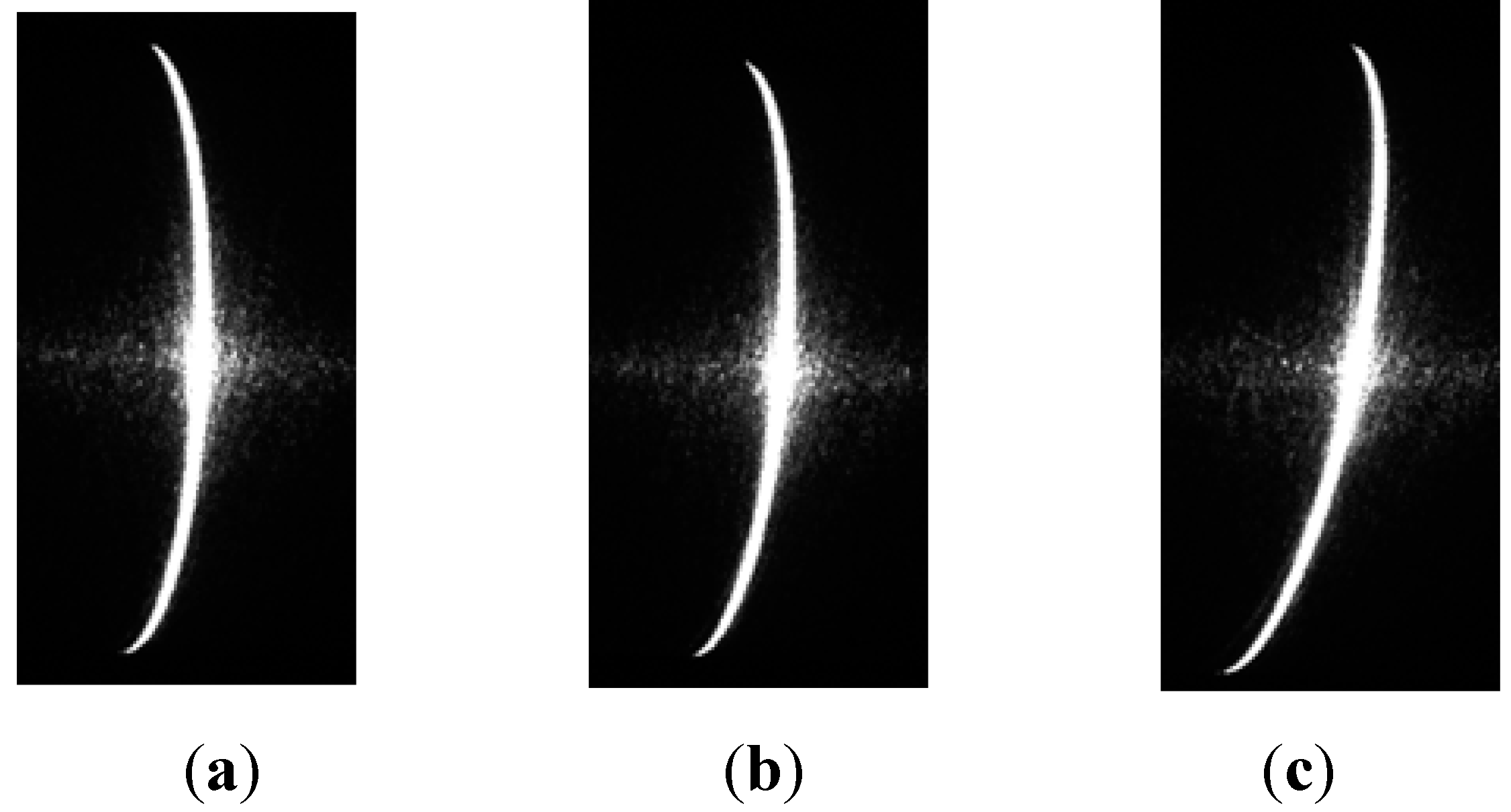
From Table 7 and Table 8, the light angle appears to have very little effect on the measuring accuracy of the proposed method.
| NO. | 1 | 2 | 3 | 4 | Mean Error |
|---|---|---|---|---|---|
| a/Errors | 0.012 | 0.011 | 0.009 | 0.004 | 0.009 |
| b/Errors | 0.014 | 0.012 | 0.012 | 0.012 | 0.013 |
| c/Errors | 0.01 | 0.016 | 0.013 | 0.008 | 0.012 |
| NO. | 1 | 2 | 3 | 4 | 5 | 6 | 7 | Mean Error |
|---|---|---|---|---|---|---|---|---|
| a/Errors | 0.008 | 0.003 | 0.017 | 0.018 | 0.025 | 0.009 | 0.022 | 0.015 |
| b/Errors | 0.005 | 0.007 | 0.004 | 0.016 | 0.026 | 0.013 | 0.018 | 0.013 |
| c/Errors | 0.008 | 0.013 | 0.025 | 0.017 | 0.028 | 0.009 | 0.022 | 0.017 |
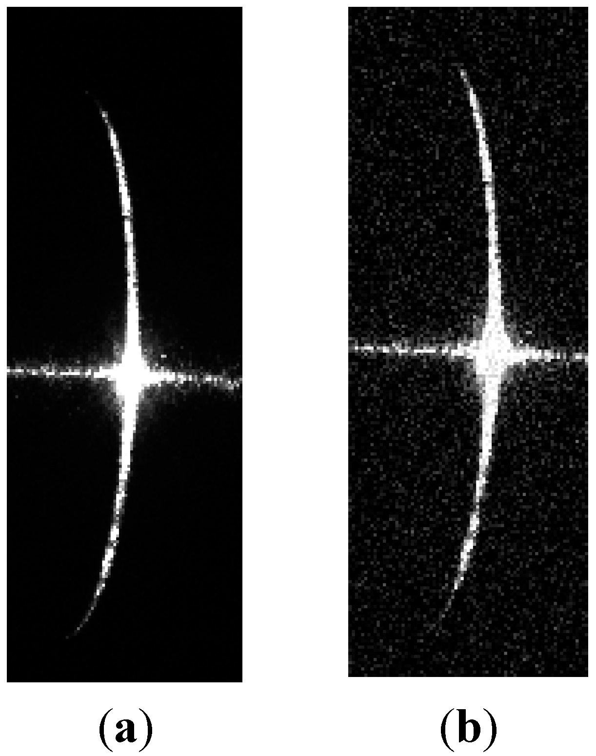
In order to test the influence of noise on the proposed method, noise with a variance of 0.01 and a mean of zero was added to the stripe images of shaft 1 and shaft 2, as shown in Figure 13 and Figure 14. The center coordinates of the stripe images with the added noise were extracted by Steger’s algorithm [14]. The shaft diameters can be determined respectively by the ellipse, circle, and the proposed method fitting the center coordinates. The results are listed in Table 9 and Figure 10.
Figure 13.
Images of stripe on shaft 1. (a) normal; (b) added noise.
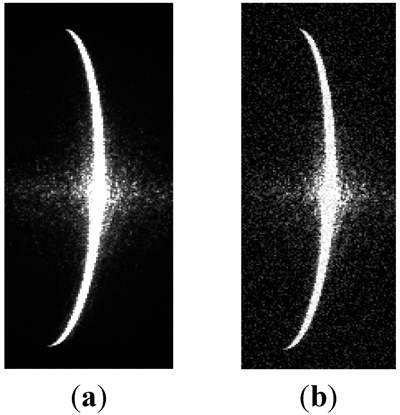
Figure 14.
Images of stripe on shaft 2. (a) normal; (b) added noise.

| D | Fitting Ellipse | Fitting Circle | Present Method | ||||
|---|---|---|---|---|---|---|---|
| D1 | Errors | D2 | Errors | D3 | Errors | ||
| Normal | 34.924 | 34.924 | 0.151 | 34.827 | 0.097 | 34.915 | 0.012 |
| Added noise | 34.924 | 34.896 | 0.028 | 34.837 | 0.087 | 34.918 | 0.006 |
| 0.123 | 0.01 | 0.003 | |||||
| D | Fitting Ellipse | Fitting Circle | Present Method | ||||
|---|---|---|---|---|---|---|---|
| D1 | Errors | D2 | Errors | D3 | Errors | ||
| Normal | 31.473 | 30.877 | 0.596 | 31.395 | 0.078 | 31.456 | 0.017 |
| Added noise | 31.473 | 30.762 | 0.711 | 31.421 | 0.052 | 31.47 | 0.003 |
| 0.115 | 0.026 | 0.014 | |||||
5. Conclusions
A method for the measurement of shaft diameters is proposed which is based on a structured light vision measurement. A virtual plane is established perpendicular to the measured shaft axis and an equation for the virtual plane is determined using a calibrated model of structured light measurement. To improve the measurement accuracy, the center of the measured shaft can be obtained by fitting the projected light stripe image on the virtual plane under the geometrical constraints. Using specific experimental conditions, measurement errors of the method were less than 25 μm and the angle between the structured light plane and the measured shaft barely affected the measurement accuracy.
Acknowledgments
The work described in this paper is partially supported by the Foundation of Jilin Provincial Education Department under Grant 201591.
Author Contributions
Siyuan Liu proposed the algorithm, designed and performed experiments, and wrote the initial manuscript. Qingchang Tan conducted the analysis of the algorithm. Yachao Zhang performed experiments.
Conflicts of Interest
The authors declare no conflicts of interest.
Appendix A
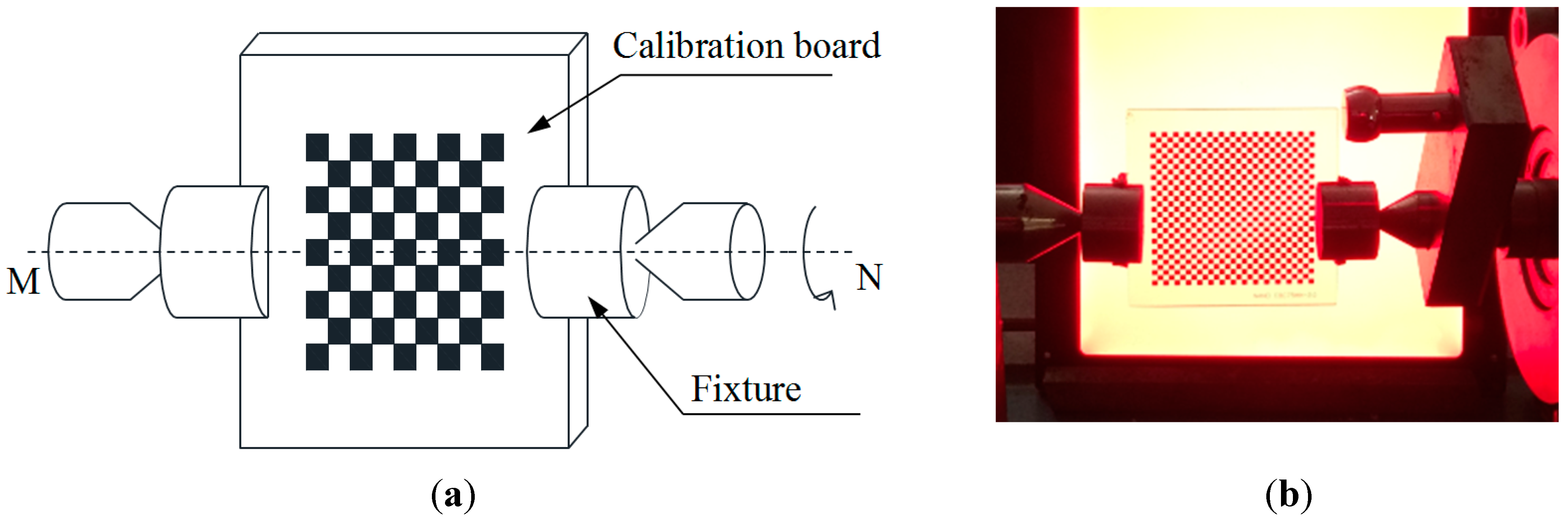
Since the virtual plane п2 is perpendicular to the measured shaft, the direction vector of the axis is the normal vector of п2. As shown in Figure A1, the calibration board is fixed by fixtures, and they are clamped by the two centers and the connecting line of the two centers is the axis of the shaft MN. Turning the calibration board, the images of the board can be captured by a camera and MN is the intersecting line of the calibration board planes.
Figure A1.
The model of the calibrating axis. (a) sketch map; (b) image of equipment.
Based on Equation (1), Equation (A1) can be obtained:
Set to , where, Rj and tj are the rotation matrix and translation vector of the calibration target at the jth position and can be obtained by the method provided in Section 2, j = 1,2. Since world coordinate systems OjWXjWYjWZjW are built on the calibration target plane, Zjw = 0. The equation of the calibration target plane at the jth position is:
The normal vector of the plane is . MN is the intersecting line of the two planes, so the direction vector of MN can be represented as:
As shown in Figure 6, Or is a point in п2 and set Or is the intersection point of MN and п1, and the camera coordinate of Or is Or = (Xr,Yr,Zr).
The equation of п2 in OCXCYCZC is
Thus, equation parameters of the virtual plane can be obtained using Equations (9) and (A4):
Appendix B
are the points for circle fitting, and the coordinates can be obtained by Equation (17). The coordinates are substituted into Equation (12). Then Equation (12) is handled by the principle of least squares as:
where, , , .
Using obtained by Equation (B1), the measured shaft diameter can be obtained by Equation (13).
The coordinates of points for ellipse fitting are . To facilitate the ellipse fitting, a new coordinate system is established on the structured light plane п1, and the camera coordinates can be converted into in the coordinate system. The coordinates are substituted into Equation (10). Then Equation (10) is handled by the principle of least squares as:
where, , , .
Using obtained by Equation (B2), the measured shaft diameter can be obtained by Equation (11).
Since the matrixes (A1, A2) and the vectors (b1,b2) in Equations (B1) and (B2) consist of the coordinates of the light stripe centers, the matrixes and vectors are influenced by errors of the light stripe centers’ coordinates, which show that and are inaccurate. From Numerical Analysis (Seventh Edition) by Burden and Faires [15], the influence is analyzed as shown below.
Considering the errors of the light stripe centers’ coordinates, matrix A1 and vector b1 in Equation (B1) are expressed as:
where and are caused by errors of the light stripe centers’ coordinates. Thus, in Equation (B1) becomes , and Equation (B1) can be expressed as:
Set is an invertible matrix, and from Equation (B4) we get:
In order to analyze the error of the fitting circle equation’s parameters, the norm of Equation (B5) is:
where is error of the circle equation’s parameters obtained by the circle fitting.
In the same way, the error of the equation’s parameters for the ellipse fitting can be obtained by Equation (B2)
From Equations (B1) and (B2), and can be calculated by the light stripe centers’ coordinates.
When the measured shaft diameter is 24.753 mm, and can be calculated by the coordinates of the light stripe centers.
So
From Equations (B8) and (B9), must be very small if . From Equation (B4), cannot be a zero vector. So, a very small requires that the absolute values of elements in the matrices and the vector must be very small. This shows that the errors of the light stripe centers’ coordinates for the ellipse fitting must be smaller than the ones for the circle fitting. On the other hand, if the coordinate errors of the light stripe centers for the circle fitting are the same as those for the ellipse fitting, the error of the circle equation parameters obtained by the circle fitting is smaller than the one of the ellipse equation parameters obtained by the ellipse fitting. From Equations (11) and (13), the measuring accuracy of the shaft diameter by circle fitting is better than by ellipse fitting. When the measured shaft diameter is 27.664 mm, and , the same results can be obtained.
References
- Takesa, K.; Sato, H.; Tani, Y.; Sata, T. Measurement of diameter using charge coupled device (CCD). CIRP Ann. Manuf. Technol. 1984, 33, 377–381. [Google Scholar] [CrossRef]
- Butler, D.J.; Forbes, G.W. Fiber-diameter measurement by occlusion of a Gaussian beam. Appl. Opt. 1998, 37, 2598–2607. [Google Scholar] [CrossRef] [PubMed]
- Lemeshko, Y.A.; Chugui, Y.V.; Yarovaya, A.K. Precision dimensional inspection of diameters of circular reflecting cylinders. Optoelectron. Instrum. Data Process 2007, 43, 284–291. [Google Scholar] [CrossRef]
- Xu, Y.; Sasaki, O.; Suzuki, T. Double-grating interferometer for measurement of cylinder diameters. Appl. Opt. 2004, 43, 537–541. [Google Scholar] [CrossRef] [PubMed]
- Song, Q.; Zhu, S.; Yan, H.; Wu, W. Signal processing method of the diameter measurement system based on CCD parallel light projection method. Proc. SPIE 2007, 6829. [Google Scholar] [CrossRef]
- Wei, G.; Tan, Q. Measurement of shaft diameters by machine vision. Appl. Opt. 2011, 50, 3246–3253. [Google Scholar] [CrossRef] [PubMed]
- Sun, Q.; Hou, Y.; Tan, Q. A Planar-Dimensions Machine Vision Measurement Method Based on Lens Distortion Correction. Sci. World J. Opt. 2013, 2013, 1–6. [Google Scholar] [CrossRef] [PubMed]
- Song, Q.; Wu, D.; Liu, J.; Zhang, C.; Huang, J. Instrumentation design and precision analysis of the external diameter measurement system based on CCD parallel light projection method. Proc. SPIE 2008, 7156. [Google Scholar] [CrossRef]
- Sun, Q.; Hou, Y.; Tan, Q.; Li, C. Shaft diameter measurement using a digital image. Opt. Lasers Eng. 2014, 55, 183–188. [Google Scholar] [CrossRef]
- Sun, Q.; You, Q.; Qiu, Y.; Ye, S. Online machine vision method for measuring the diameter and straightness of seamless steel pipes. Opt. Eng. 2001, 40, 2565–2571. [Google Scholar] [CrossRef]
- Liu, B.; Wang, P.; Zeng, Y.; Sun, C. Measuring method for micro-diameter based on structured-light vision technology. Chin. Opt. Lett. 2009, 8, 666–669. [Google Scholar]
- Zhang, Z. A flexible new technique for camera calibration. IEEE Trans. Pattern Anal. Mach. Intell. 2000, 22, 1330–1334. [Google Scholar] [CrossRef]
- More, J. The Levenberg-Marquardt Algorithm, Implementation and Theory. In Numerical Analysis; Springer: Berlin, Germany, 1977. [Google Scholar]
- Steger, C. An unbiased detector of curvilinear structures. IEEE Trans. Pattern Anal. Mach. Intell. 1998, 20, 113–125. [Google Scholar] [CrossRef]
- Burden, R.L.; Faires, J.D. Numerical Analysis, 7th ed.; Thomson Learning: Belmont, CA, USA, 2001; p. 461. [Google Scholar]
© 2015 by the authors; licensee MDPI, Basel, Switzerland. This article is an open access article distributed under the terms and conditions of the Creative Commons Attribution license (http://creativecommons.org/licenses/by/4.0/).
Share and Cite
MDPI and ACS Style
Liu, S.; Tan, Q.; Zhang, Y. Shaft Diameter Measurement Using Structured Light Vision. Sensors 2015, 15, 19750-19767. https://doi.org/10.3390/s150819750
AMA Style
Liu S, Tan Q, Zhang Y. Shaft Diameter Measurement Using Structured Light Vision. Sensors. 2015; 15(8):19750-19767. https://doi.org/10.3390/s150819750
Chicago/Turabian StyleLiu, Siyuan, Qingchang Tan, and Yachao Zhang. 2015. "Shaft Diameter Measurement Using Structured Light Vision" Sensors 15, no. 8: 19750-19767. https://doi.org/10.3390/s150819750