
Radar Imaging of Non-Uniformly Rotating Targets via a Novel Approach for Multi-Component AM-FM Signal Parameter Estimation

Abstract
:1. Introduction
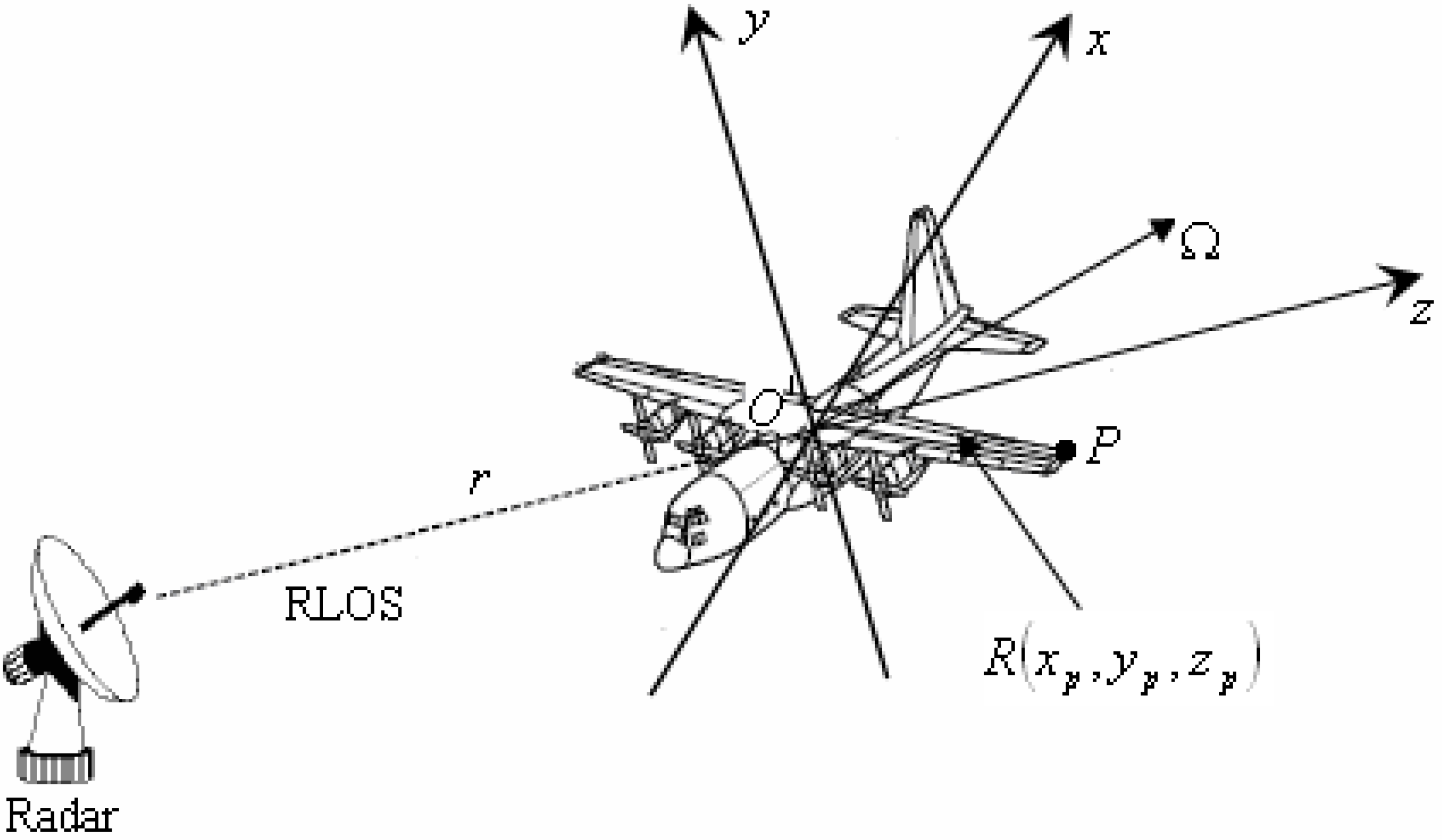
2. Signal Model

3. Modified Version of Chirplet Decomposition Based on IHAF
3.1. Principle of Modified Version of Chirplet Decomposition

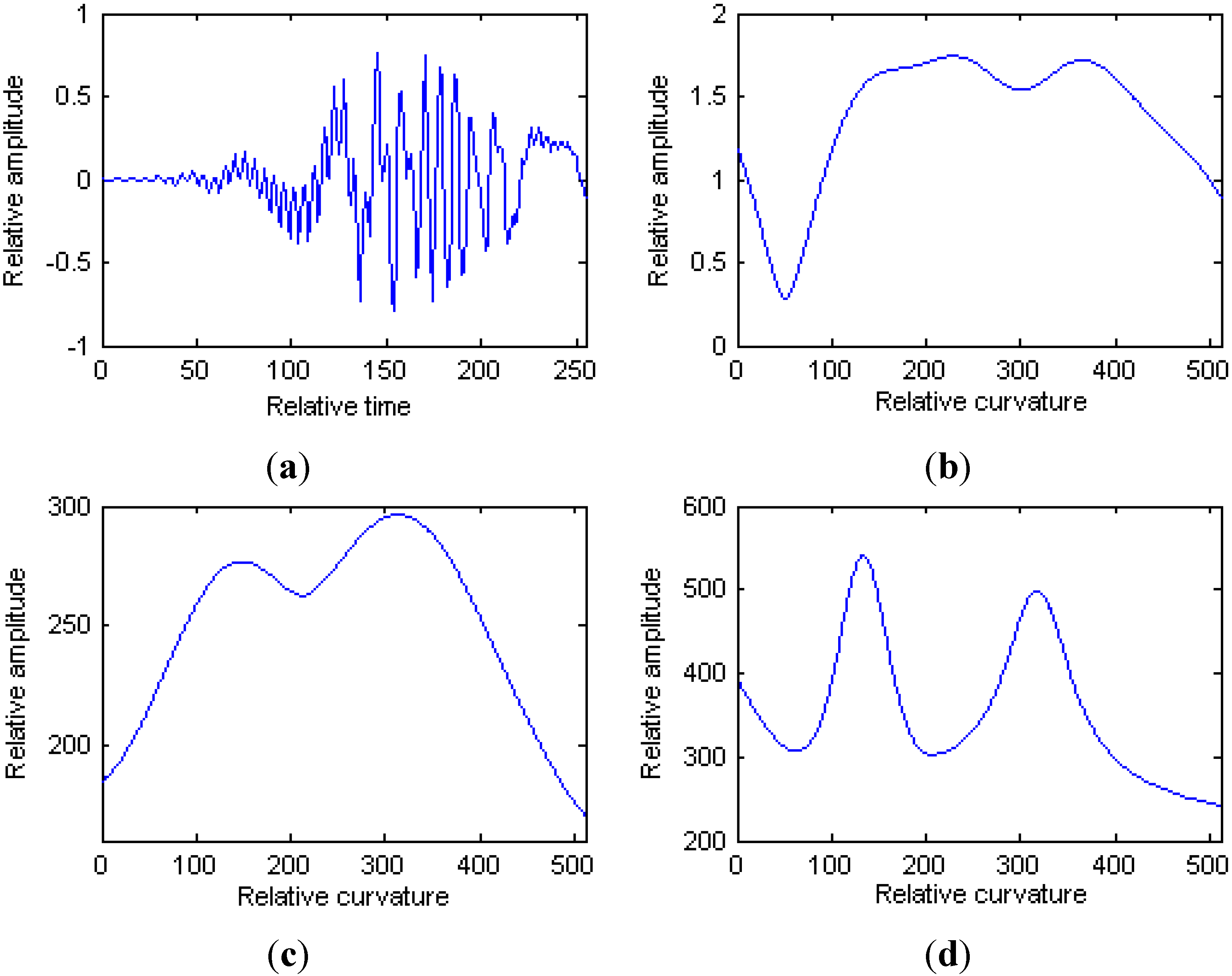
3.2. Modified Version of Chirplet Decomposition Based on IHAF
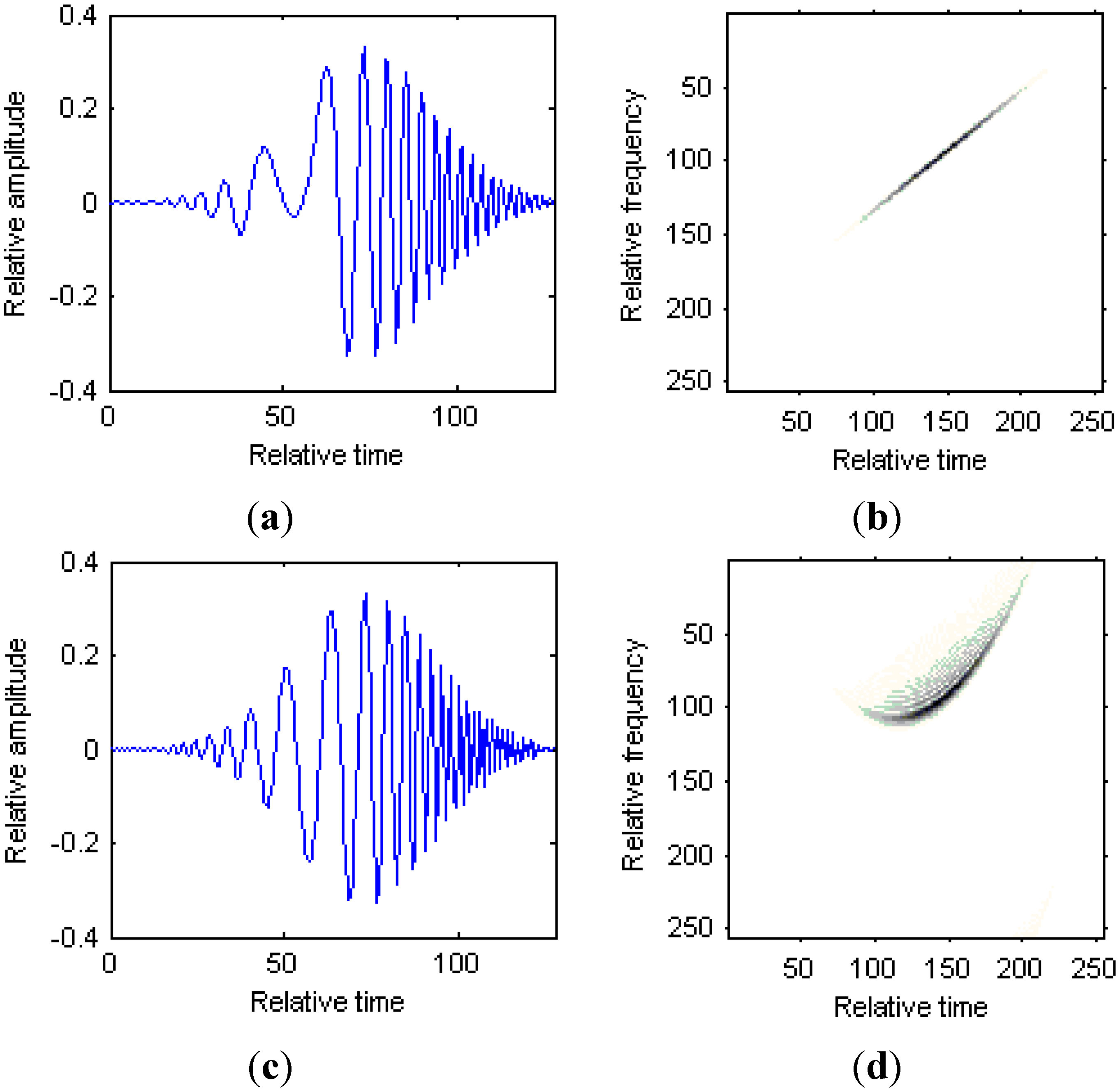
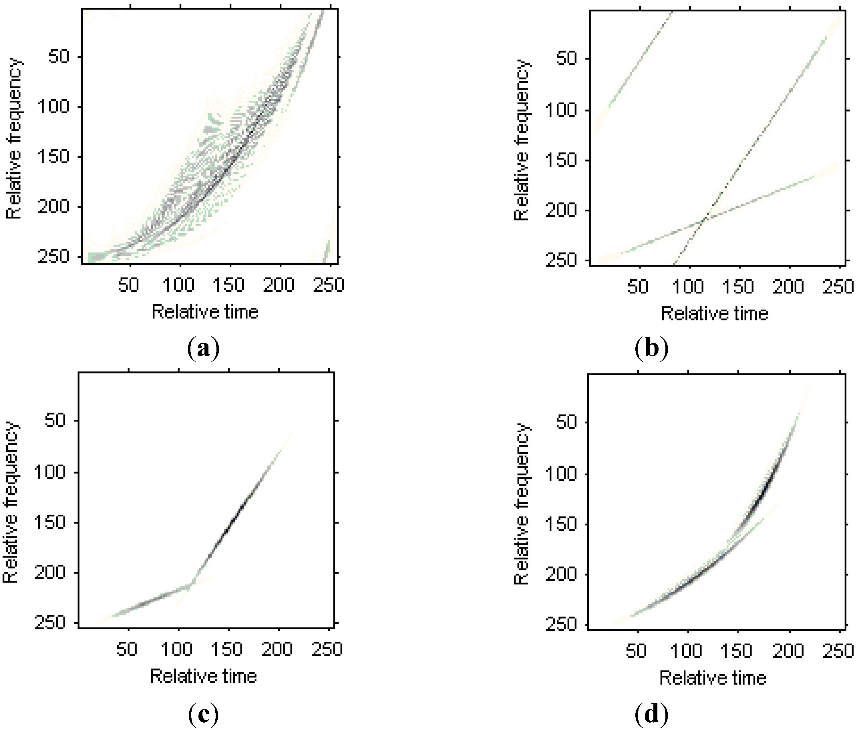
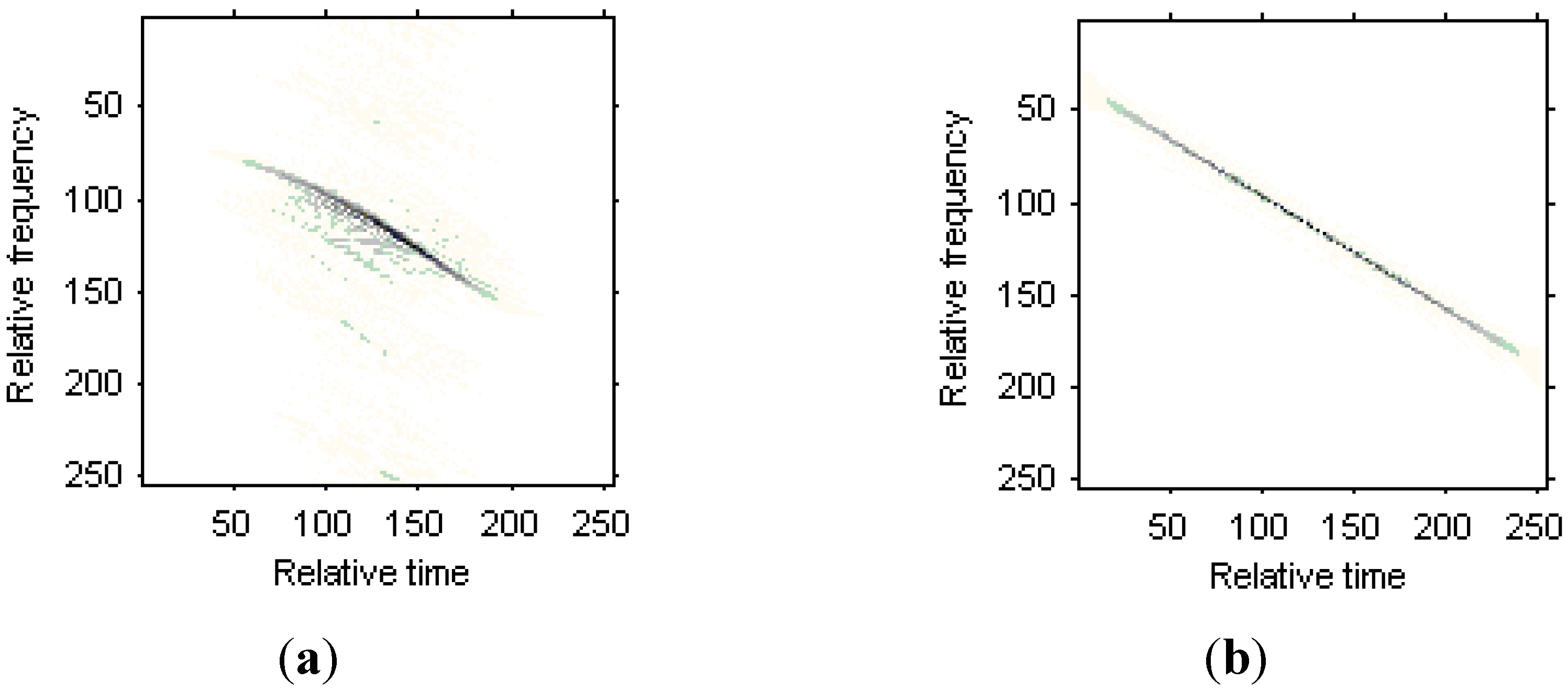
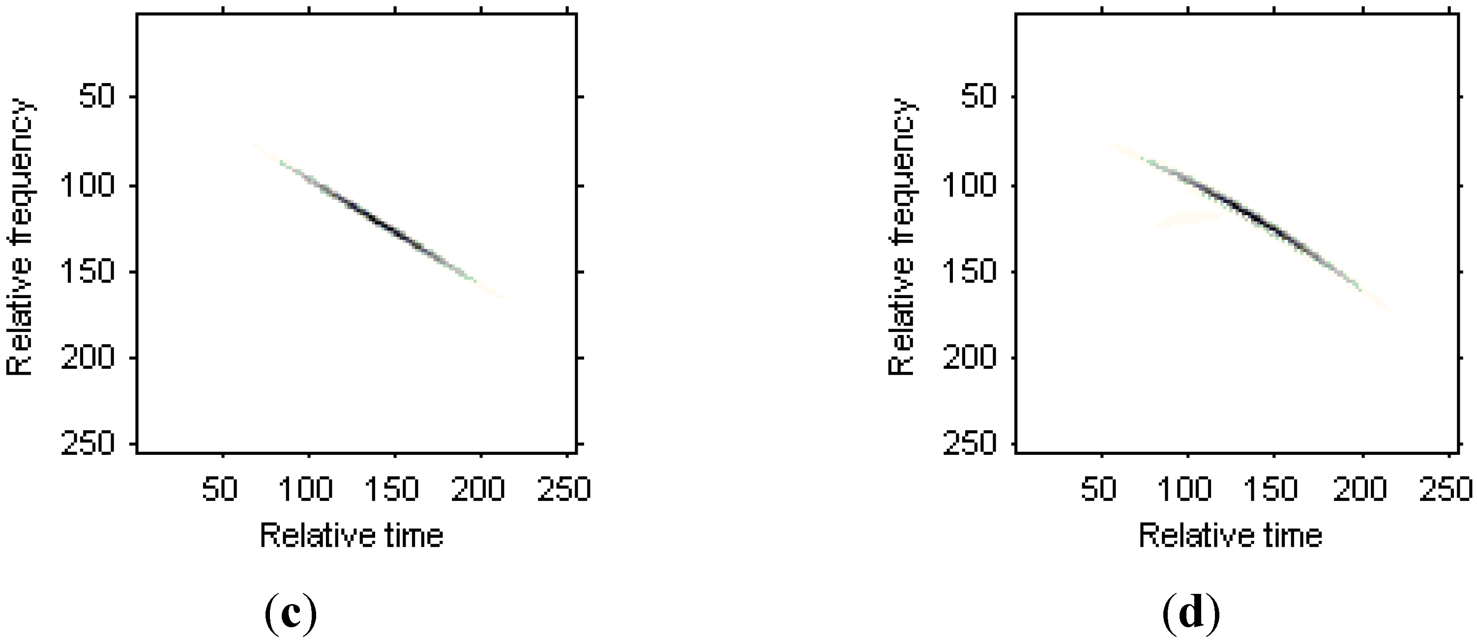
3.3. Numerical Example

| Components (k) | Dk | σk | tk | ωk | βk | γk |
|---|---|---|---|---|---|---|
| 1 | 4 | 40 | 18 | 0.4 | 5×10⁻³ | 1×10⁻⁵ |
| 2 | 4 | 60 | 50 | 0.8 | −5×10⁻³ | −2×10⁻⁵ |

4. Radar Imaging Based on Modified Version of Chirplet Decomposition
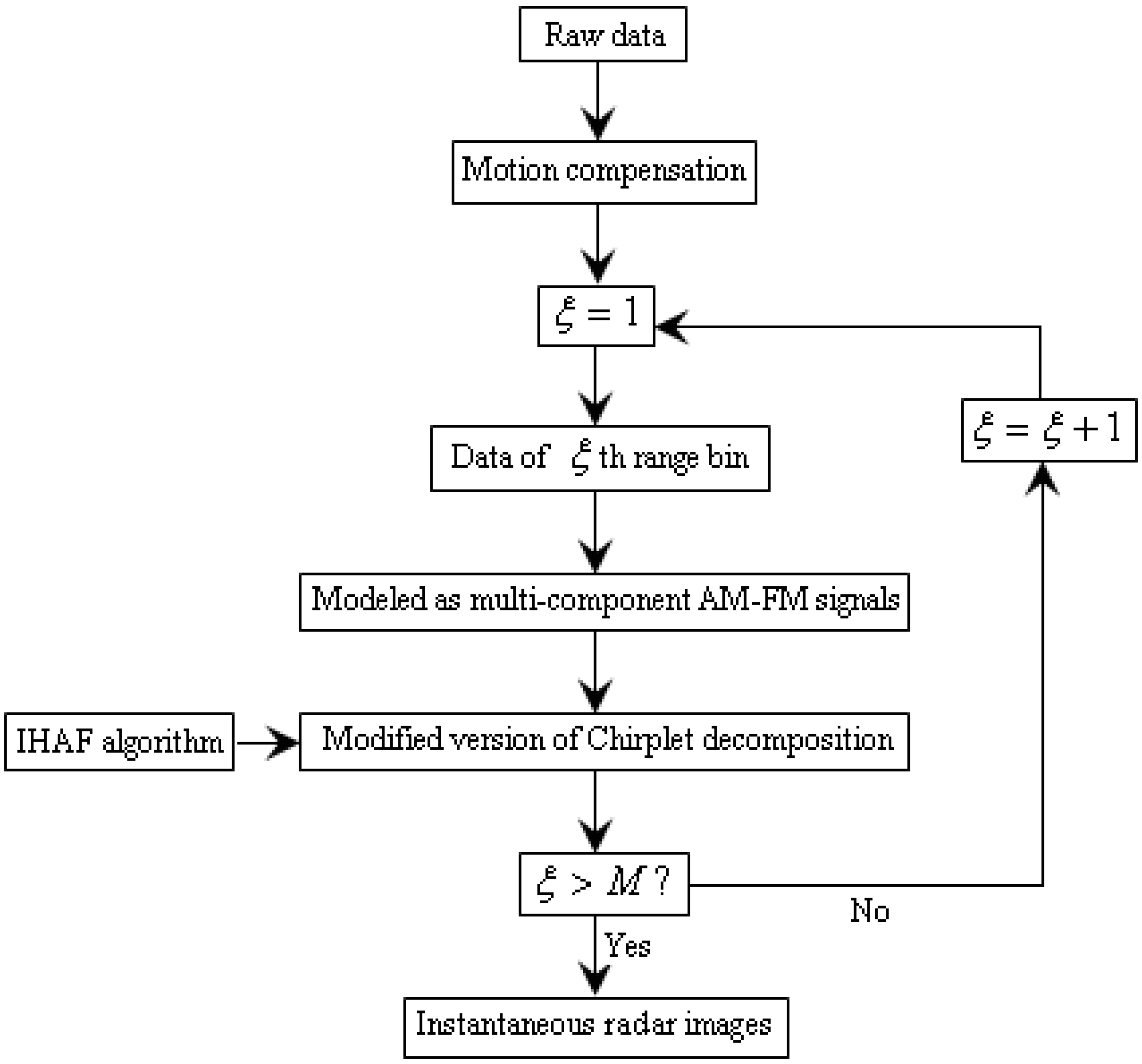
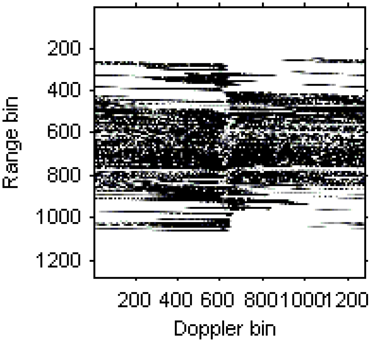
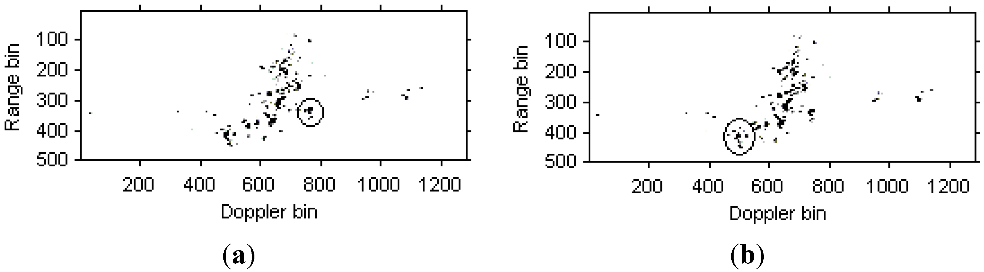
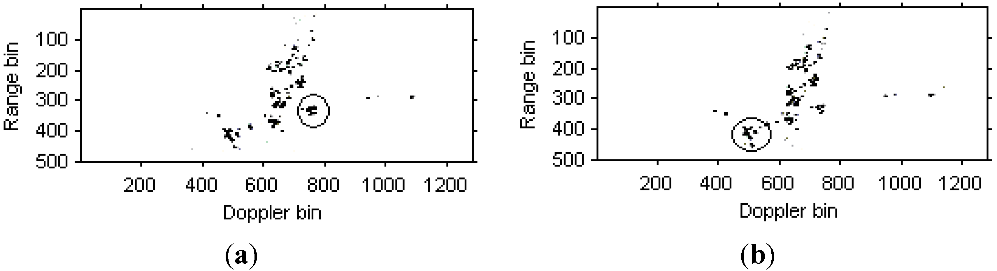
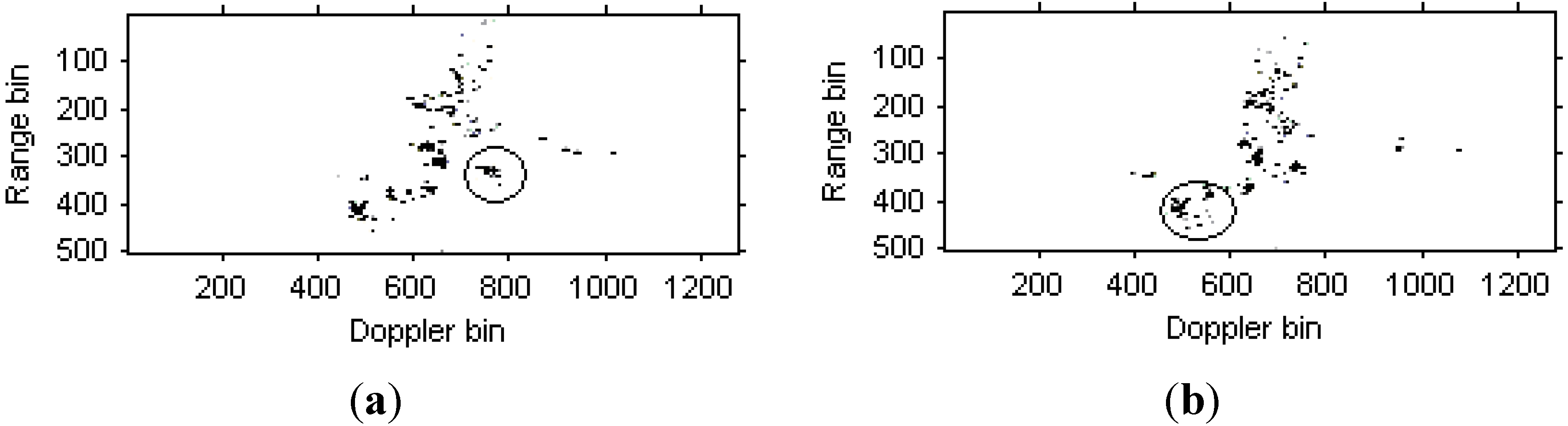
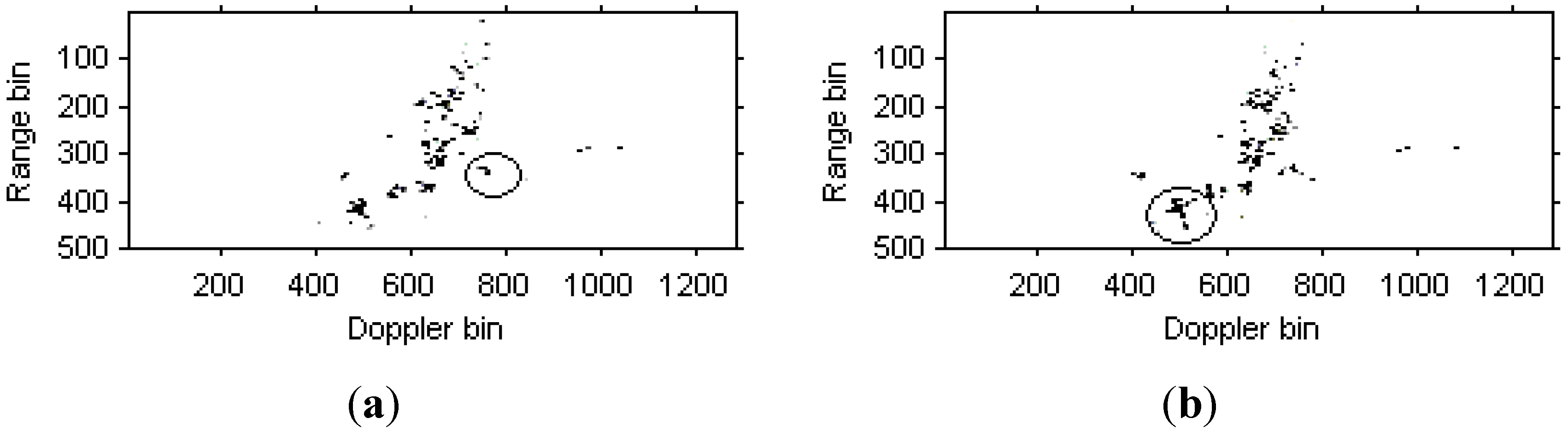
5. Radar Imaging Results
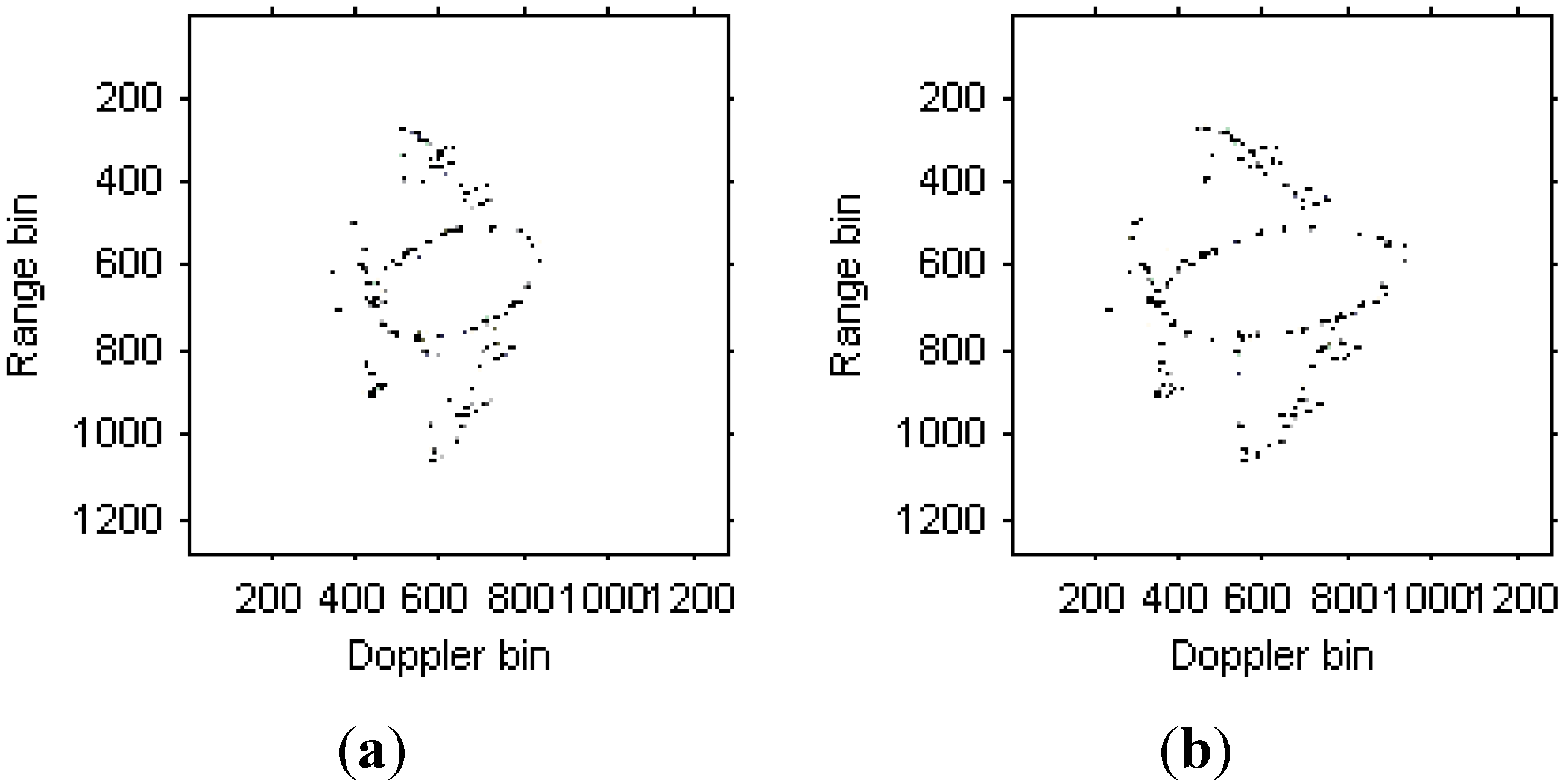
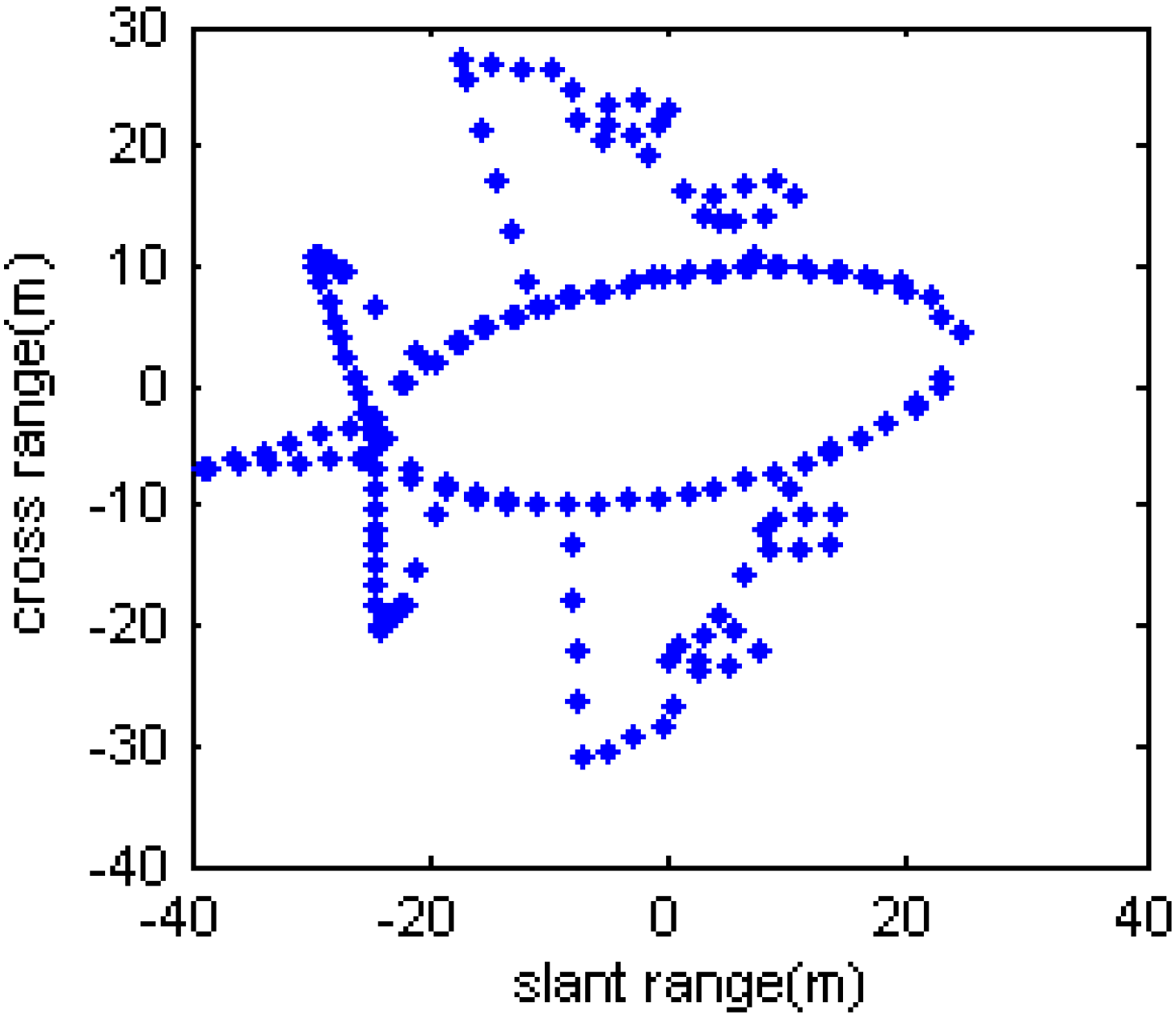
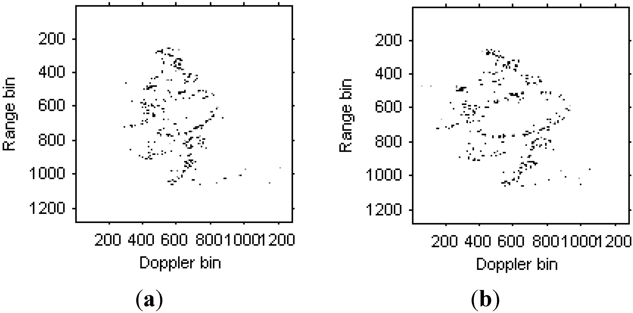
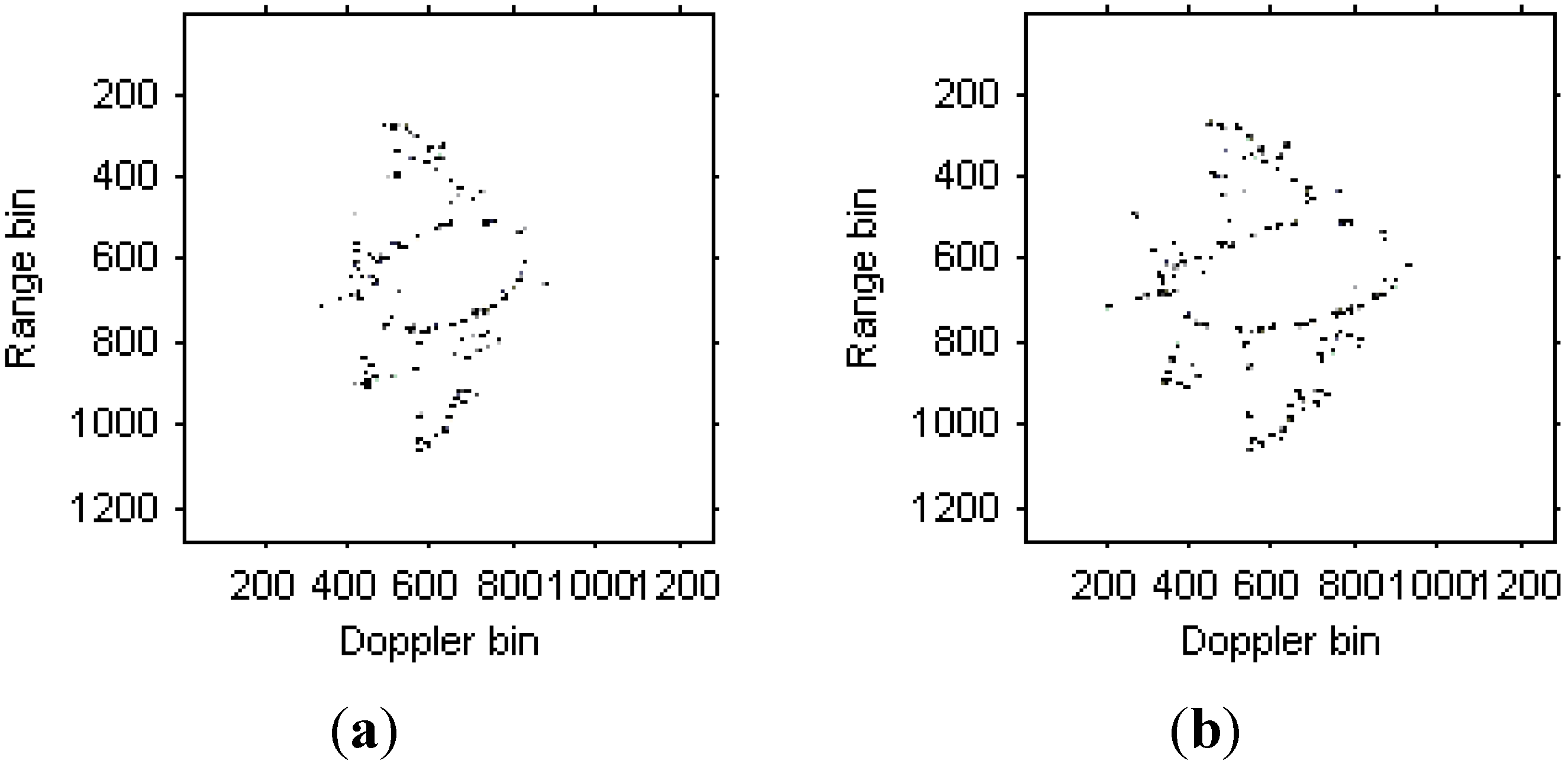
5.1. Simulated Data


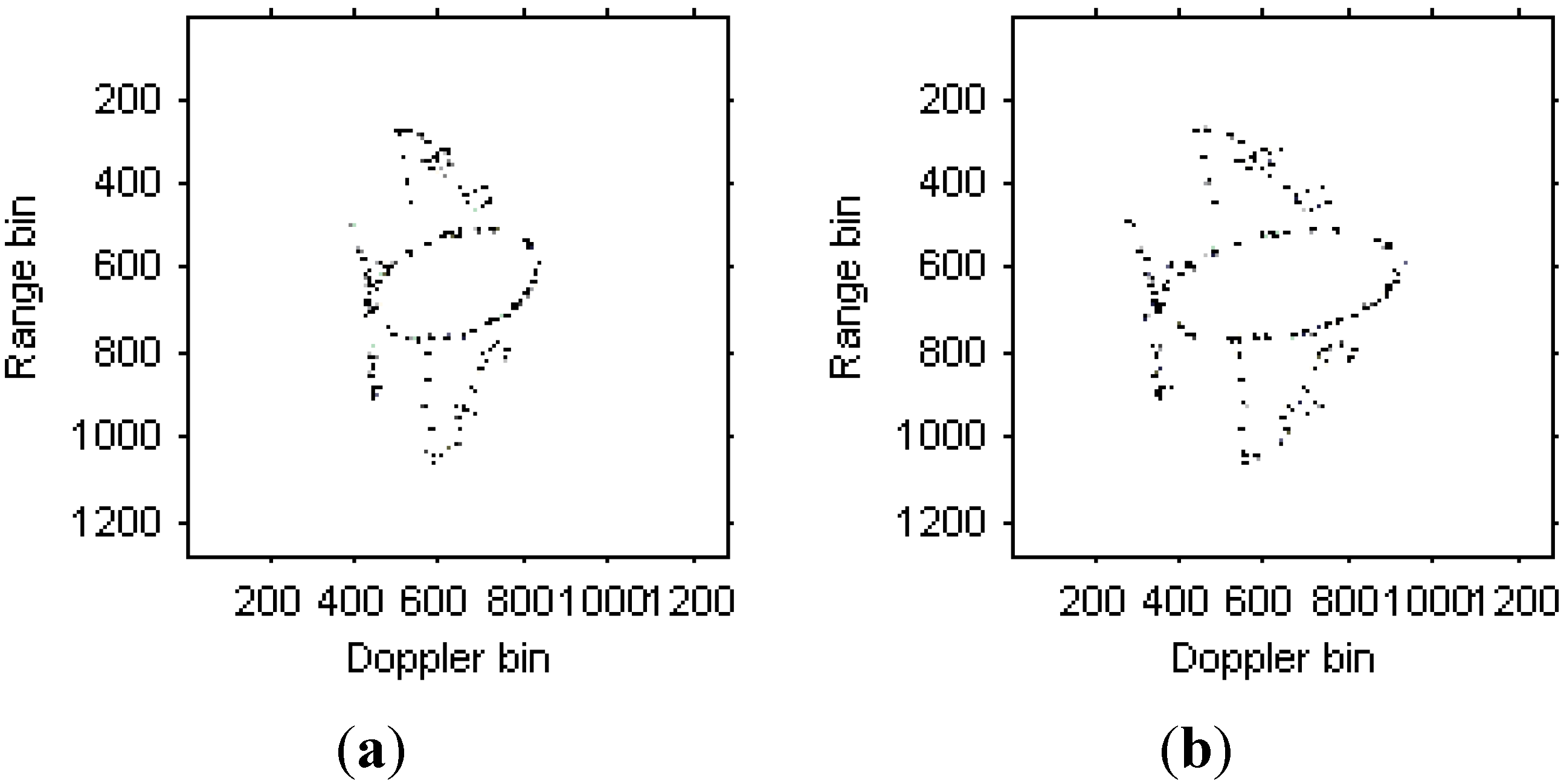
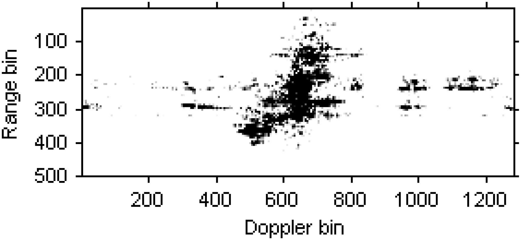
5.2. Real Data


6. Conclusions
Acknowledgements
Nomenclature
| O | Rotating center of the target |
| r | Unit vector of the RLOS |
| × | Outer product |
| ● | Inner product |
| P | Random scatterer on the target |
| λ | Wavelength |
| Ω | Synthetic vector for the angular velocity of the rotating target |
| K | Polynomial phase order |
| α0 | Constant term |
| R0 | Initial distance from radar to the target center |
| t0 | Initial time |
| Q | Number of scatterers in a range cell |
| tk | Time center of the modified version of Chirplet atom |
| ωk | Frequency center of the modified version of Chirplet atom |
| βk | Chirp rate of the modified version of Chirplet atom |
| γk | Curvature of the modified version of Chirplet atom |
| σk | Width for the modified version of Chirplet atom |
| Ck | Weighted coefficient |
| (⋅)∗ | Conjugate |
| m1 | Time lags |
| m2 | Time lags |
Conflicts of Interest
References
- Berizzi, F.; Mese, E.D.; Diani, M.; Martorella, M. High-resolution ISAR imaging of maneuvering targets by means of the range instantaneous Doppler technique: Modeling and performance analysis. IEEE Trans. Image Process. 2001, 10, 1880–1890. [Google Scholar] [CrossRef] [PubMed]
- Zheng, J.B.; Su, T.; Zhu, W.T.; Liu, Q.H.; Zhang, L.; Zhu, T.W. Fast parameter estimation algorithm for cubic phase signal based on quantifying effects of Doppler frequency shift. Prog. Electromagn. Res. 2013, 142, 57–74. [Google Scholar] [CrossRef]
- Bao, Z.; Wang, G.Y.; Luo, L. Inverse synthetic aperture radar imaging of maneuvering targets. Opt. Eng. 1998, 37, 1582–1588. [Google Scholar] [CrossRef]
- Li, Z.; Narayanan, R.M. Manoeuvring target motion parameter estimation for ISAR image fusion. IET Signal Process. 2008, 2, 325–334. [Google Scholar] [CrossRef]
- Chen, V.C.; Miceli, W.J. Time-varying spectral analysis for radar imaging of maneuvering targets. IEE Proc. Radar Sonar Navig. 1998, 145, 262–268. [Google Scholar] [CrossRef]
- Li, G.; Zhang, H.; Wang, X.Q.; Xia, X.G. ISAR 2-D imaging of uniformly rotating targets via matching pursuit. IEEE Trans. AES 2012, 48, 1838–1846. [Google Scholar]
- Walker, J.L. Range-Doppler imaging of rotating objects. IEEE Trans. AES 1980, 16, 23–52. [Google Scholar]
- Sanchez, M.P.; Guasp, M.R.; Antonino-Daviu, J.A.; Folch, J.R.; Cruz, J.P.; Panadero, R.P. Instantaneous frequency of the left sideband harmonic during the start-up transient: A new method for diagnosis of broken bars. IEEE Trans. Ind. Electron. 2009, 56, 4557–4570. [Google Scholar] [CrossRef]
- Santos, F.V.; Guasp, M.R.; Henao, H.; Sanchez, M.P.; Panadero, R.P. Diagnosis of rotor and stator asymmetries in wound-rotor induction machines under nonstationary operation through the instantaneous frequency. IEEE Trans. Ind. Electron. 2014, 61, 4947–4959. [Google Scholar] [CrossRef]
- Cohen, L. Time-Frequency distributions——A review. IEEE Proc. 1989, 77, 941–981. [Google Scholar] [CrossRef]
- Wang, Y.; Jiang, Y.C. ISAR imaging of maneuvering target based on the L-Class of fourth order complex-Lag PWVD. IEEE Trans. Geosci. Remote Sens. 2010, 48, 1518–1527. [Google Scholar] [CrossRef]
- Stankovic, L. L-class of time-frequency distributions. IEEE Signal Process. Lett. 1996, 3, 22–25. [Google Scholar] [CrossRef]
- Stankovic, L.; Thayaparan, T.; Dakovic, M. Signal decomposition by using the S-Method with application to the analysis of HF radar signals in sea-clutter. IEEE Trans. Signal Process. 2006, 54, 4332–4342. [Google Scholar] [CrossRef]
- Wang, Y.; Jiang, Y.C. Inverse synthetic aperture radar imaging of three-dimensional rotation target based on two-order match Fourier transform. IET Signal Process. 2012, 6, 159–169. [Google Scholar] [CrossRef]
- Bai, X.; Tao, R.; Wang, Z.J.; Wang, Y. ISAR imaging of a ship target based on parameter estimation of multicomponent quadratic frequency-modulated signals. IEEE Trans. Geosci. Remote Sens. 2014, 52, 1418–1429. [Google Scholar] [CrossRef]
- Zheng, J.B.; Su, T.; Zhu, W.T.; Liu, Q.H. ISAR imaging of targets with complex motions based on the keystone time-chirp rate distribution. IEEE Geosci. Remote Sens. Lett. 2014, 11, 1275–1279. [Google Scholar] [CrossRef]
- Zheng, J.B.; Su, T.; Zhang, L.; Zhu, W.T.; Liu, Q.H. ISAR imaging of targets with complex motion based on the chirp rate-quadratic chirp rate distribution. IEEE Trans. Geosci. Remote Sens. 2014, 52, 7276–7289. [Google Scholar] [CrossRef]
- Wang, Y. Inverse synthetic aperture radar imaging of manoeuvring target based on range-instantaneous-Doppler and range-instantaneous-chirp-rate algorithms. IET Radar Sonar Navig. 2012, 6, 921–928. [Google Scholar] [CrossRef]
- Bultan, A. A four-parameter atomic decomposition of chirplets. IEEE Trans. Signal Process. 1999, 47, 731–745. [Google Scholar] [CrossRef]
- Yin, Q.Y.; Qian, S.; Feng, A.G. A fast refinement for adaptive Gaussian chirplet decomposition. IEEE Trans. Signal Process. 2002, 50, 1298–1306. [Google Scholar] [CrossRef]
- Greenberg, J.M.; Wang, Z.S.; Li, J. New approaches for chirplet approximation. IEEE Trans. Signal Process. 2007, 55, 734–741. [Google Scholar] [CrossRef]
- Wang, Y.; Jiang, Y.C. ISAR imaging for three-dimensional rotation targets based on adaptive Chirplet decomposition. Multidimens. Syst. Signal Process. 2010, 21, 59–71. [Google Scholar] [CrossRef]
- Angrisani, L.; D’Arco, M. A measurement method based on a modified version of the Chirplet transform for instantaneous frequency estimation. IEEE Trans. Instrument. Meas. 2002, 51, 704–711. [Google Scholar] [CrossRef]
- Yang, Y.; Zhang, W.M.; Peng, Z.K.; Meng, G. Multicomponent signal analysis based on polynomial Chirplet transform. IEEE Trans. Ind. Electron. 2013, 60, 3948–3956. [Google Scholar] [CrossRef]
- Wang, Y.; Jiang, Y.C. Modified adaptive Chirplet decomposition with application in ISAR imaging of maneuvering targets. EURASIP J. Adv. Signal Process. 2008. [CrossRef]
- Yang, Y.; Peng, Z.K.; Meng, G.; Zhang, W.M. Spline-kernelled Chirplet transform for the analysis of signals with time-varying frequency and its application. IEEE Trans. Ind. Electron. 2012, 59, 1612–1621. [Google Scholar] [CrossRef]
- Barbarossa, S.; Petrone, V. Analysis of polynomial-phase signals by the integrated generalized ambiguity function. IEEE Trans. Signal Process. 1997, 45, 316–327. [Google Scholar] [CrossRef]
- Gough, P.T. A fast spectral estimation algorithm based on the FFT. IEEE Trans. Signal Process. 1994, 42, 1317–1322. [Google Scholar] [CrossRef]
- Wang, P.; Li, H.B.; Djurovic, I.; Himed, B. Integrated cubic phase function for linear FM signal analysis. IEEE Trans. Aerosp. Electron. Syst. 2010, 46, 963–977. [Google Scholar] [CrossRef]
- Wang, Y.; Jiang, Y.C. Approach for high resolution inverse synthetic aperture radar imaging of ship target with complex motion. IET Signal Process. 2013, 7, 146–157. [Google Scholar] [CrossRef]
- Wang, Y.; Zhao, B.; Jiang, Y.C. Inverse synthetic aperture radar imaging of targets with complex motion based on cubic Chirplet decomposition. IET Signal Process. 2015. accepted. [Google Scholar]
- Wang, J.F.; Liu, X.Z. Improved global range alignment for ISAR. IEEE Trans. Aerosp. Electron. Syst. 2007, 43, 1070–1075. [Google Scholar] [CrossRef]
© 2015 by the authors; licensee MDPI, Basel, Switzerland. This article is an open access article distributed under the terms and conditions of the Creative Commons Attribution license (http://creativecommons.org/licenses/by/4.0/).
Share and Cite
Wang, Y. Radar Imaging of Non-Uniformly Rotating Targets via a Novel Approach for Multi-Component AM-FM Signal Parameter Estimation. Sensors 2015, 15, 6905-6923. https://doi.org/10.3390/s150306905
Wang Y. Radar Imaging of Non-Uniformly Rotating Targets via a Novel Approach for Multi-Component AM-FM Signal Parameter Estimation. Sensors. 2015; 15(3):6905-6923. https://doi.org/10.3390/s150306905
Chicago/Turabian StyleWang, Yong. 2015. "Radar Imaging of Non-Uniformly Rotating Targets via a Novel Approach for Multi-Component AM-FM Signal Parameter Estimation" Sensors 15, no. 3: 6905-6923. https://doi.org/10.3390/s150306905