
A Timing Estimation Method Based-on Skewness Analysis in Vehicular Wireless Networks


Abstract
:1. Introduction
- (1)
- A new cross-correlation, summing up and skewness analysis (denoted CSS) method is proposed which can be used to estimate the time offset in positioning sensors of vehicular wireless networks.
- (2)
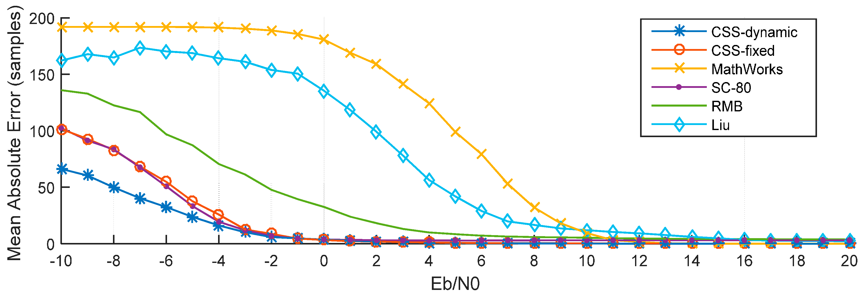
- The CSS method provides better precision than some well-known time estimation techniques, especially in low signal to noise ratio (SNR), and multi-path environments, which is very important for vehicular wireless networks.
- (3)
- The CSS method can also be used in other wireless communications which use OFDM with repeated preamble symbols, such as IEEE 802.11a.
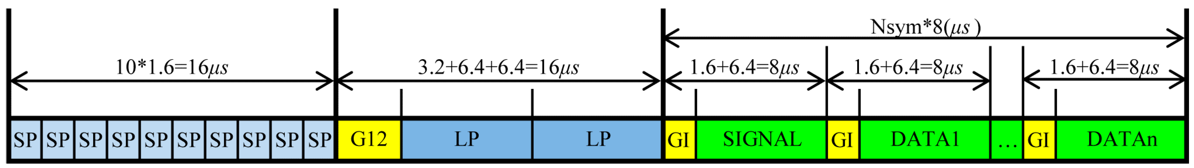
2. OFDM Preamble Structure
2.1. Modulation Technique
2.2. Preamble Symbols

3. Related Work
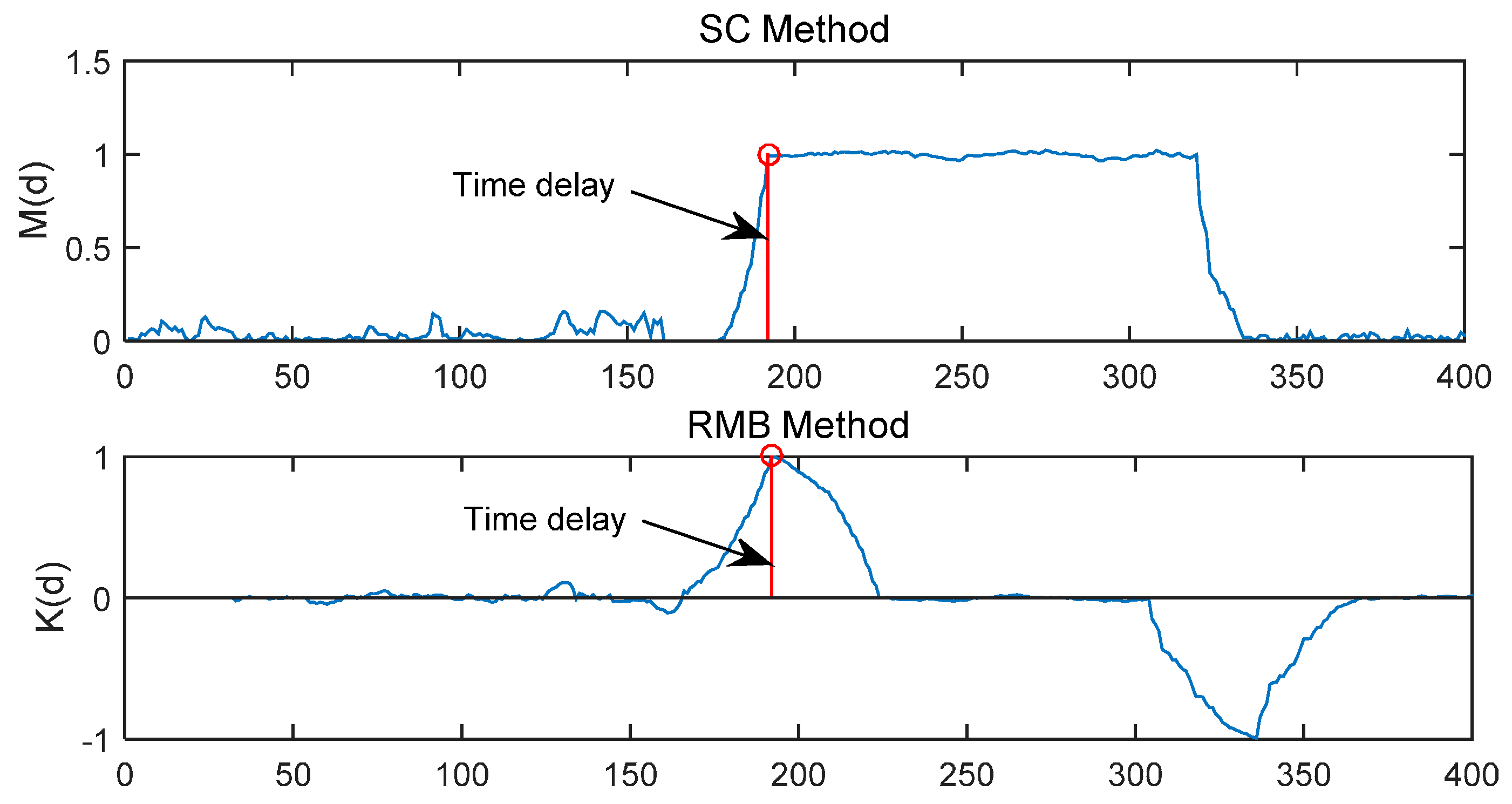
3.1. SC Method

3.2. RMB Method

3.3. MathWorks Method

3.4. Liu et al. Method

4. Proposed Timing Estimation Method
4.1. Cross-Correlation
4.2. Summing-Up


4.3. Skewness-Analysis and Threshold
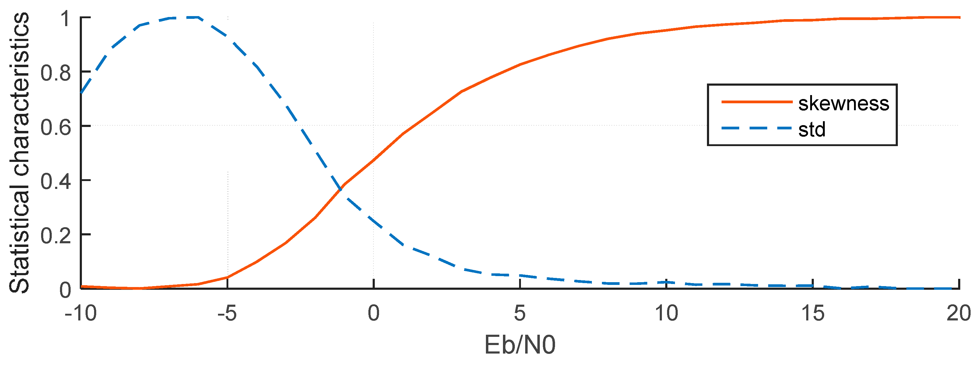
4.3.1 Statistical Characteristics of the Summing-Up Samples
- (1)
- Standard Deviation
- (2)
- Skewness

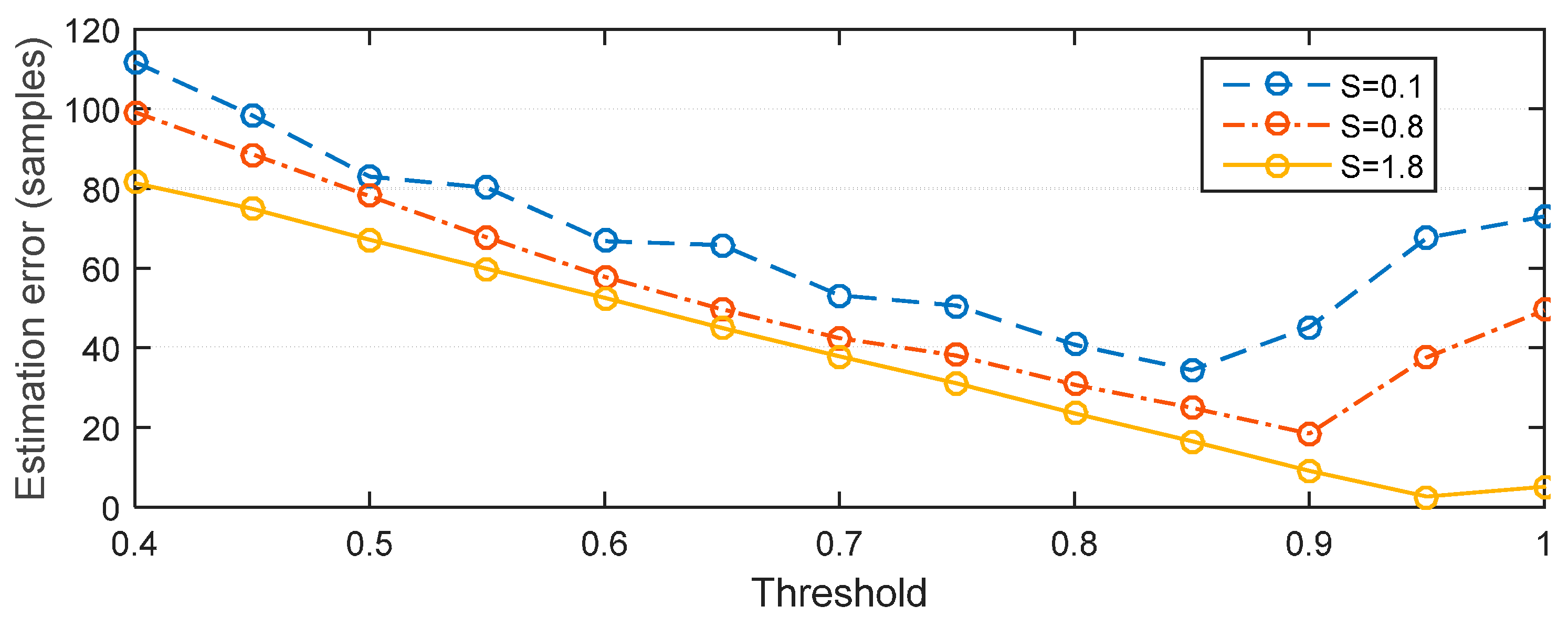
4.3.2. Relationship between Estimation Error, Skewness and Threshold

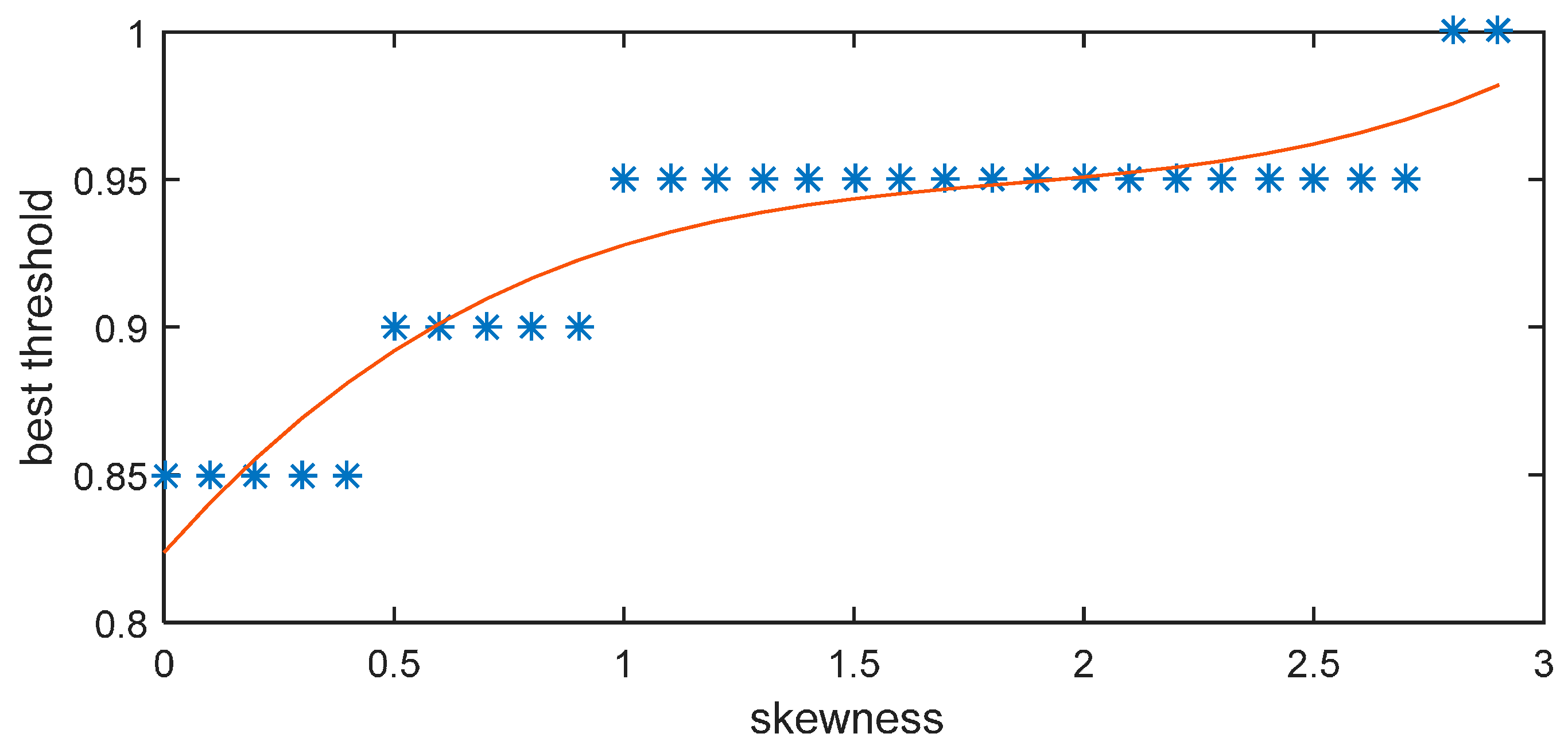
4.3.3. Relationship between Skewness and Threshold

5. Simulation Setup and Result Analysis
5.1. Simulation Setup
5.1.1. System Model


| Parameters | Value |
|---|---|
| Modulation mode | BPSK |
| Number of subcarriers | 52 |
| Symbol duration | 8 μs |
| Guard time | 1.6 μs |
| FFT period | 6.4 μs |
| Preamble duration | 32 μs |
| Subcarrier spacing | 0.15625 MHz |
| Vehicle speed | 100 km/h |
| Channel mode | ITU-A |
5.1.2. Transmission Channel
| Tap | Channel A | Channel B | Doppler | ||
|---|---|---|---|---|---|
| Relative Delay (ns) | Average Power (dB) | Relative Delay (ns) | Average Power (dB) | Spectrum | |
| 1 | 0 | 0.0 | 0 | –2.5 | Classic |
| 2 | 310 | –1.0 | 300 | 0 | Classic |
| 3 | 710 | –9.0 | 8900 | –12.8 | Classic |
| 4 | 1090 | –10.0 | 12,900 | –10.0 | Classic |
| 5 | 1730 | –15.0 | 17,100 | –25.2 | Classic |
| 6 | 2510 | –20.0 | 20,000 | –16.0 | Classic |
5.1.3. Performance Metric
5.2. Performance Results and Analysis
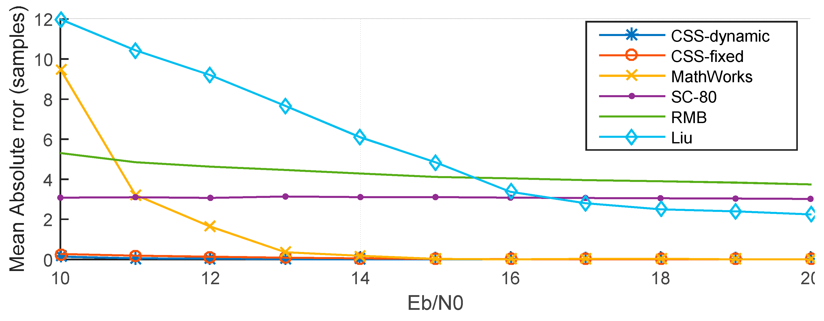
5.2.1. Estimation Error

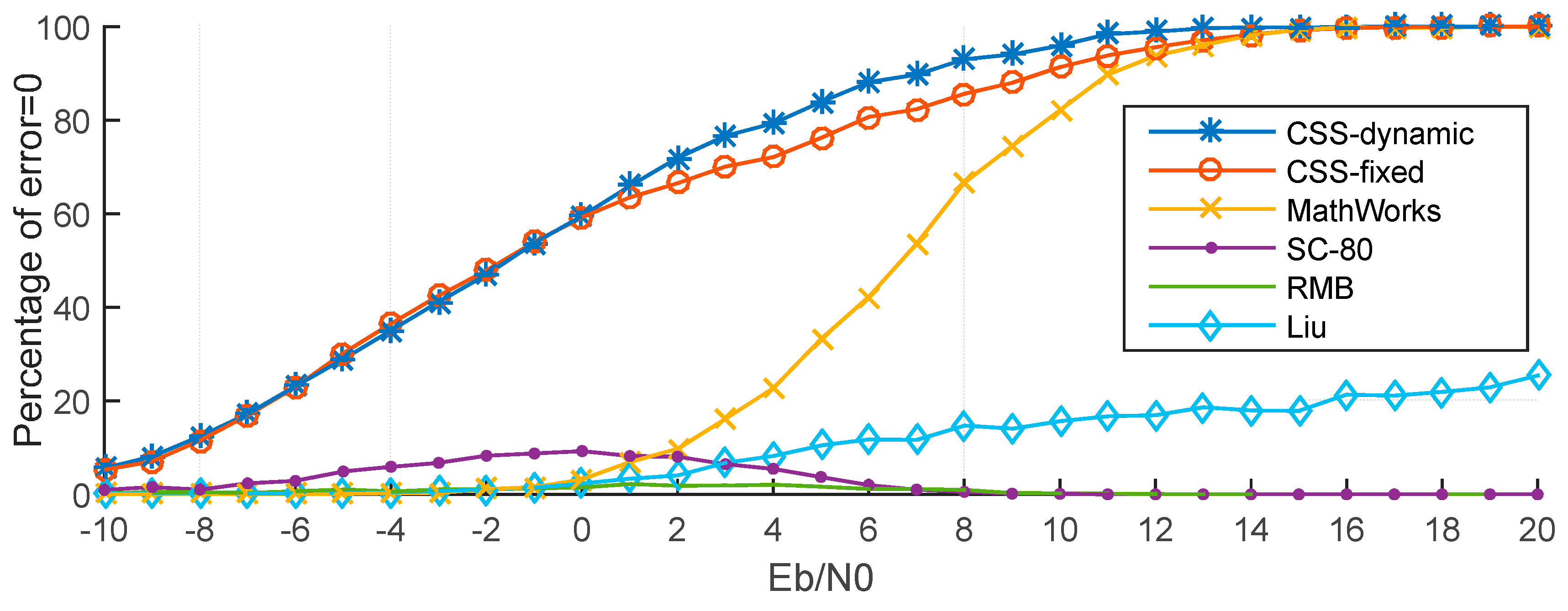
5.2.2. Correct Percentage
- (1)
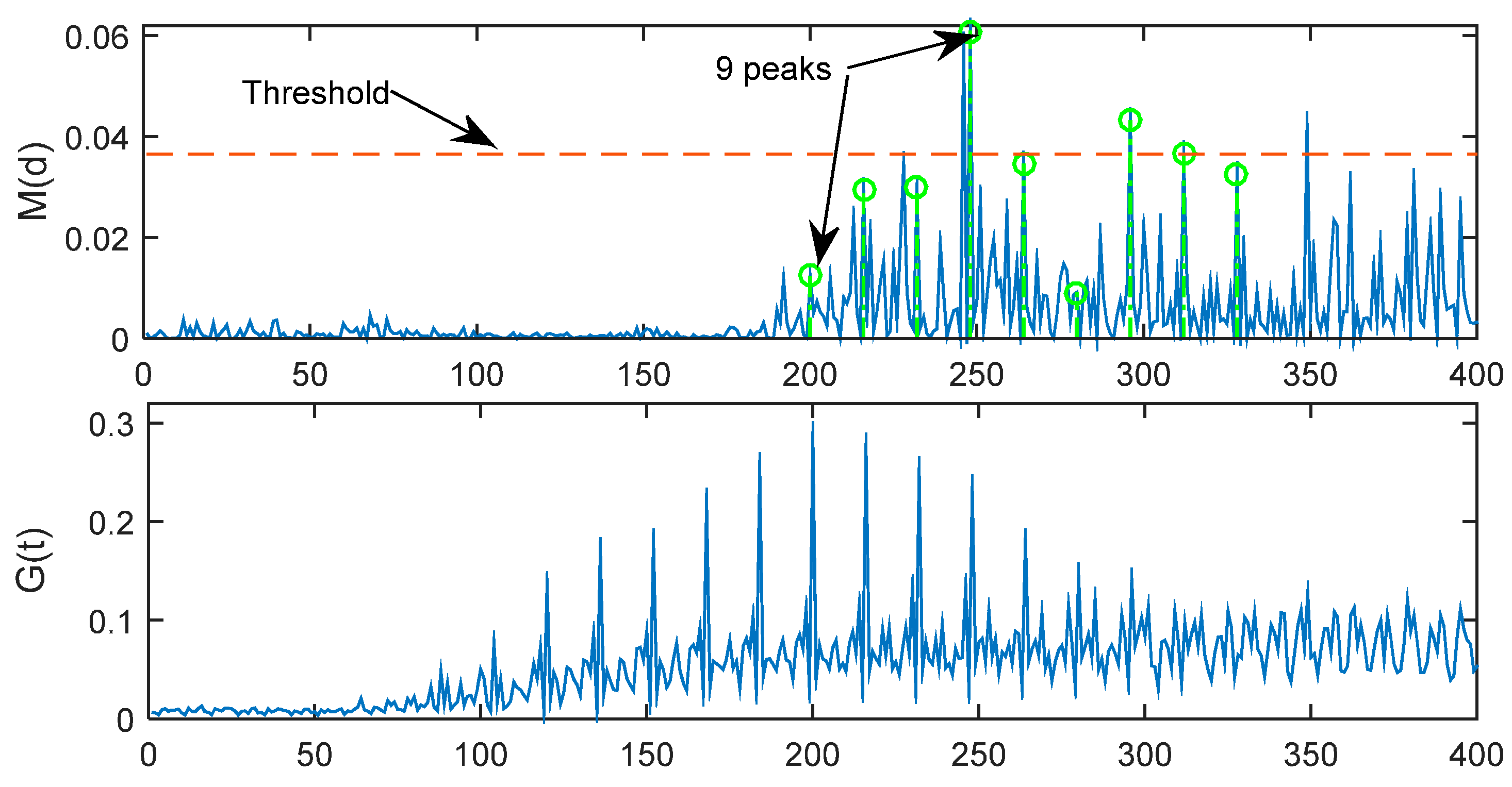
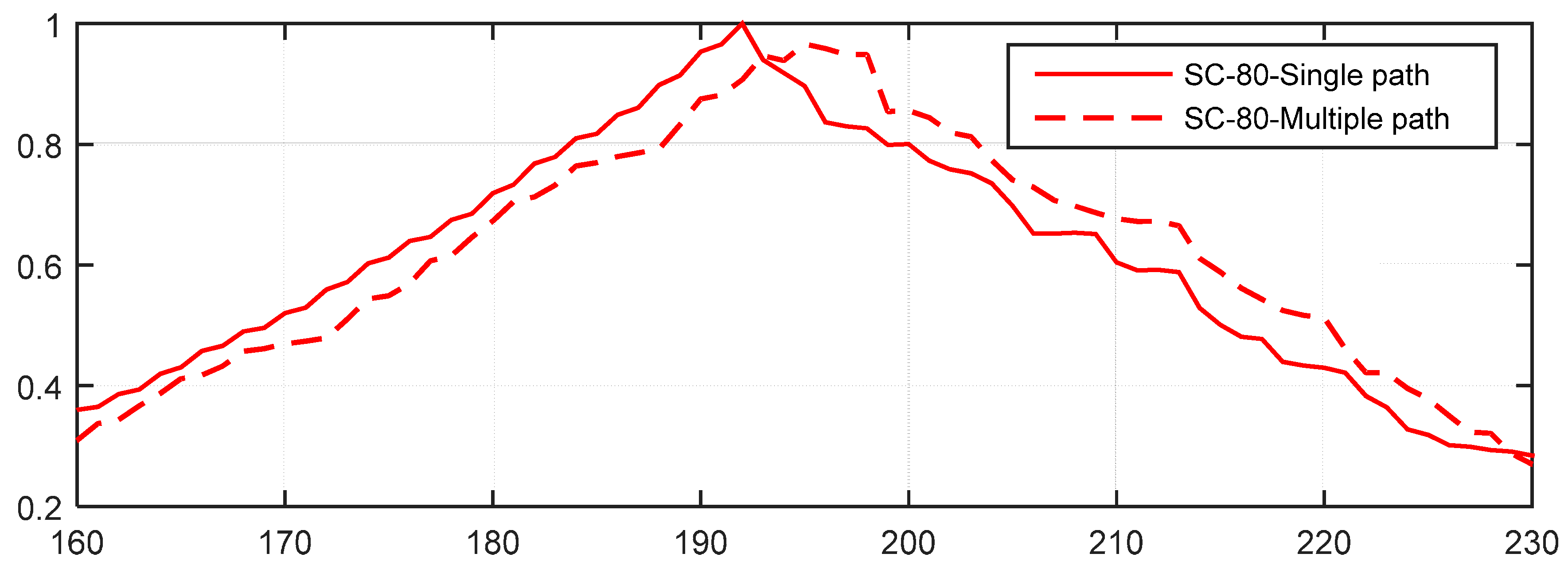
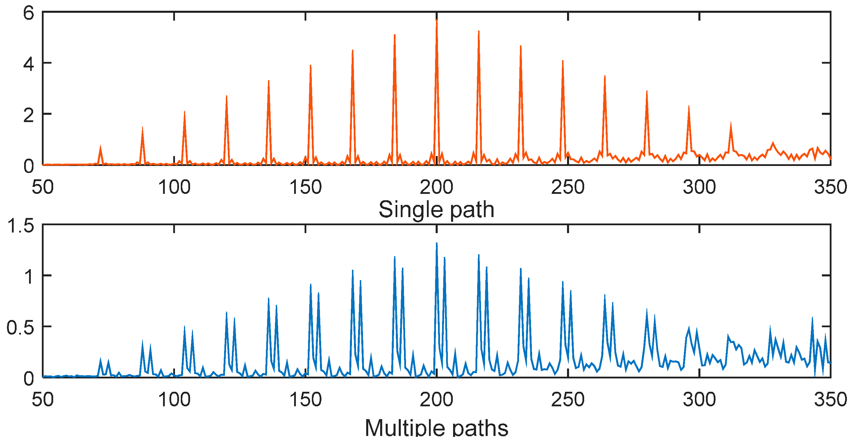
- When Eb/N0 is high, the multipath in the ITU channel causes the peaks to move to the right, making the timing estimation incorrect. Take the SC-80 method as an example, which is illustrated in Figure 16. The percentage will be close to 0 but will not reach 0. On the other hand, Figure 17 gives the corresponding results for the CSS method. This shows that the maximum peak with the CSS method does not move in the multipath channel, and only some smaller peaks are generated, so the percentage will be nearly equal to 100% for a high Eb/N0.
- (2)
- When Eb/N0 is very low (close to −10 dB), the noise levels are too high, so it is too difficult to locate the peak, so the percentage is again close to 0.
- (3)
- For Eb/N0 around 0 dB, the signal energy is close to that of the noise, so it is easier to locate the peak. Now because of the randomization of noise, it’s likely that the estimated time happens to be the true time delayed.


6. Conclusions
Acknowledgments
Author Contributions
Conflicts of Interest
References
- World Health Organization. Global Status Report on Road Safety 2013: Supporting a Decade of Action. Available online: http://www.who.int/iris/bitstream/10665/78256/1/9789241564564_eng.pdf (accessed on 30 August 2015).
- Xiao, Z.; Bai, J.; Ma, G.Y.; Fan, J.T.; Yi, K.C. Research on positioning enhancement scheme of CAPS via UWB pseudolite. Sci. China Phys. Mech. Astron. 2012, 55, 733–737. [Google Scholar] [CrossRef]
- Ansari, K.; Feng, Y.M.; Tang, M.L. A runtime integrity monitoring framework for real-time relative positioning systems based on GPS and DSRC. IEEE Trans. Intell. Transp. Syst. 2015, 16, 980–992. [Google Scholar] [CrossRef]
- IEEE 802.11p-2010 Standard. Available online: http://standards.ieee.org/getieee802/download/802.11p-2010.pdf (accessed on 30 August 2015).
- Haijun, Z.; Chunxiao, J.; Julian, C. Cooperative interference mitigation and handover management for heterogeneous cloud small cell networks. IEEE Wirel. Commun. 2015, 22, 92–99. [Google Scholar] [CrossRef]
- Wei, W.; Qi, Y. Information potential fields navigation in wireless Ad-Hoc sensor networks. Sensors 2011, 11, 4794–4807. [Google Scholar] [CrossRef] [PubMed]
- Sanchez-Rodriguez, D.; Hernandez-Morera, P.; Quinteiro, J.M.; Alonso-Gonzalez, I. A low complexity system based on multiple weighted decision trees for indoor localization. Sensors 2015, 15, 14809–14829. [Google Scholar] [CrossRef] [PubMed]
- Vera, R.; Ochoa, S.F.; Aldunate, R.G. EDIPS: an easy to deploy indoor positioning system to support loosely coupled mobile work. Pers. Ubiquit. Comput. 2011, 15, 365–376. [Google Scholar] [CrossRef]
- IEEE 802.11a-1999 Standard. Available online: http://standards.ieee.org/getieee802/download/802.11a-1999.pdf (accessed on 30 August 2015).
- Cui, X.-R.; Zhang, H.; Aaron Gulliver, T. Threshold selection for ultra-wideband TOA estimation based on neural networks. J. Netw. 2012, 7, 1311–1318. [Google Scholar] [CrossRef]
- Sun, Y.L.; Xu, Y.B.; Li, C.; Ma, L. Kalman/map filtering-aided fast normalized cross correlation-based Wi-Fi fingerprinting location sensing. Sensors 2013, 13, 15513–15531. [Google Scholar] [CrossRef] [PubMed]
- Tomic, S.; Beko, M.; Dinis, R. Distributed RSS-based localization in wireless sensor networks based on second-order cone programming. Sensors 2014, 14, 18410–18432. [Google Scholar] [CrossRef] [PubMed]
- Miao, C.Y.; Dai, G.Y.; Ying, K.Z.; Chen, Q.Z. Collaborative localization and location verification in WSNs. Sensors 2015, 15, 10631–10649. [Google Scholar] [CrossRef] [PubMed]
- Zhang, Q.; Foh, C.H.; Seet, B.C.; Fong, A.C.M. Variable elasticity spring-relaxation: improving the accuracy of localization for WSNs with unknown path loss exponent. Pers. Ubiquit.Comput. 2012, 16, 929–941. [Google Scholar] [CrossRef]
- Adnan, T.; Datta, S.; MacLean, S. Efficient and accurate sensor network localization. Pers. Ubiquit. Comput. 2014, 18, 821–833. [Google Scholar] [CrossRef]
- Chen, Z.H.; Zou, H.; Jiang, H.; Zhu, Q.C.; Soh, Y.C.; Xie, L.H. Fusion of WiFi, smartphone sensors and landmarks using the Kalman filter for indoor localization. Sensors 2015, 15, 715–732. [Google Scholar] [CrossRef] [PubMed]
- Guo, J.Q.; Zhang, H.Y.; Sun, Y.C.; Bie, R.F. Square-root unscented Kalman filtering-based localization and tracking in the Internet of Things. Pers. Ubiquit. Comput. 2014, 18, 987–996. [Google Scholar] [CrossRef]
- Brida, P.; Machaj, J.; Benikovsky, J. A modular localization system as a positioning service for road transport. Sensors 2014, 14, 20274–20296. [Google Scholar] [CrossRef] [PubMed]
- Schmidl, T.M.; Cox, D.C. Robust frequency and timing synchronization for OFDM. IEEE Trans. Commun. 1997, 45, 1613–1621. [Google Scholar] [CrossRef]
- Oni, R.R.A. Preamble design problematic with 802.11a IEEE standard (Minn’s training sequence). Radioengineering 2008, 17, 87–91. [Google Scholar]
- Reddy, A.K.; Mahanta, A.A.; Bora, P.K. On timing and frequency offset estimation in OFDM systems. In Proceedings of the TENCON 2004. 2004 IEEE Region 10 Conference, 21–24 November 2004; Volume 153, pp. 153–156.
- MathWorks. OFDM Synchronization. Available online: http://www.mathworks.com/help/comm/examples/ofdm-synchronization.html (accessed on 30 August 2015).
- Yun, L.; Hua, Y.; Fei, J.; Fangjiong, C.; Weiqiang, P. Robust timing estimation method for OFDM systems with reduced complexity. IEEE Commun. Lett. 2014, 18, 1959–1962. [Google Scholar] [CrossRef]
- Guidelines for Evaluation of Radio Transmission Technologies for IMT-2000. Available online: https://www.itu.int/dms_pub/itu-r/oth/0A/0E/R0A0E00000C0001MSWE.doc (accessed on 30 August 2015).
© 2015 by the authors; licensee MDPI, Basel, Switzerland. This article is an open access article distributed under the terms and conditions of the Creative Commons Attribution license (http://creativecommons.org/licenses/by/4.0/).
Share and Cite
Cui, X.; Li, J.; Wu, C.; Liu, J.-H. A Timing Estimation Method Based-on Skewness Analysis in Vehicular Wireless Networks. Sensors 2015, 15, 28942-28959. https://doi.org/10.3390/s151128942
Cui X, Li J, Wu C, Liu J-H. A Timing Estimation Method Based-on Skewness Analysis in Vehicular Wireless Networks. Sensors. 2015; 15(11):28942-28959. https://doi.org/10.3390/s151128942
Chicago/Turabian StyleCui, Xuerong, Juan Li, Chunlei Wu, and Jian-Hang Liu. 2015. "A Timing Estimation Method Based-on Skewness Analysis in Vehicular Wireless Networks" Sensors 15, no. 11: 28942-28959. https://doi.org/10.3390/s151128942