
Observability Analysis of DVL/PS Aided INS for a Maneuvering AUV


The Acoustic and Navigation Laboratory (ANL), Department of Marine Technology, University of Haifa, Haifa 3498838, Israel
*
Author to whom correspondence should be addressed.
Sensors 2015, 15(10), 26818-26837; https://doi.org/10.3390/s151026818
Submission received: 2 September 2015
/
Revised: 6 October 2015
/
Accepted: 14 October 2015
/
Published: 22 October 2015
(This article belongs to the Section Physical Sensors)
Abstract
:Recently, ocean exploration has increased considerably through the use of autonomous underwater vehicles (AUV). A key enabling technology is the precision of the AUV navigation capability. In this paper, we focus on understanding the limitation of the AUV navigation system. That is, what are the observable error-states for different maneuvering types of the AUV? Since analyzing the performance of an underwater navigation system is highly complex, to answer the above question, current approaches use simulations. This, of course, limits the conclusions to the emulated type of vehicle used and to the simulation setup. For this reason, we take a different approach and analyze the system observability for different types of vehicle dynamics by finding the set of observable and unobservable states. To that end, we apply the observability Gramian approach, previously used only for terrestrial applications. We demonstrate our analysis for an underwater inertial navigation system aided by a Doppler velocity logger or by a pressure sensor. The result is a first prediction of the performance of an AUV standing, rotating at a position and turning at a constant speed. Our conclusions of the observable and unobservable navigation error states for different dynamics are supported by extensive numerical simulation.
1. Introduction
Recently, the use of Autonomous Underwater Vehicles (AUVs) for ocean applications has increased considerably. These applications include gathering of scientific data, pollution control, climate monitoring, transmission of images from remote places, seafloor mapping, oceanographic surveys and maintenance of off-shore facilities, to name just a few [1,2]. A typical mission of an AUV involves submerging for a few hours while following a specific route and gathering measurements with respect to the AUV’s location and dynamics. To accomplish its mission, the AUV must navigate while being submerged. Initially, the vehicle is assumed to be on the surface and location is determined, commonly, using one of the Global Navigation Satellite Systems (GNSS). However, when the vehicle is below the water surface, GNSS is no longer available and the vehicle must use its inertial system.
Advances made in the last 20 years in Inertial Navigation Systems (INS) technology, in terms of cost, size, and power consumption [3], together with the fact that INS is a standalone system, appoint the INS as the main sensor for AUV navigation. However, the INS navigation solution drifts with time due to error sources within its inertial sensor measurements. A common performance is a navigation error of about 2 km per hour for a navigation grade INS [4]. For that reason, INS is regularly fused with other sensors [5] or data [6] to produce a bounded navigation solution. The INS position solution is commonly aided by GNSS receivers, acoustic positioning [7,8], or imaging/ranging sonar [9]. In sonar imaging/ranging, template matching, for example, is employed where measured data is compared to a bathymetry map [10]. However, in some situations, neither of those position-aiding types is available. For example, when using GNSS receivers, the vehicle is required to surface. In addition, acoustic poisoning requires deploying transponders at known locations, which for most AUV applications is not possible.
When the AUV lacks position updates for some portion of time, it may obtain velocity updates from a Doppler Velocity Logger (DVL) [11,12,13], and an altitude update from a Pressure Sensor (PS) [14,15]. The measured data is introduced to a navigation filter, commonly a Kalman filter, which carries out the process of sensor fusion. The result is a solution for the navigation in terms of an updated parameter state vector. The latter usually includes the position of the AUV, its velocity, and its orientation. However, due to the lack of position updates, the position solution will diverge along with several other navigation states. To compensate for such state divergence, the AUV can maneuver.
It is well known that maneuvering affects the behavior of the navigation system. Among performance, maneuvering also alters the convergence/divergence characteristics of the navigation state vector [16]. While several attempts quantify the navigation performance of an AUV in various types of motion [17,18], an analytical analysis to understand the effect of maneuvering on the navigation capability has not been made. Such analysis is referred to as the “observability analysis”. That is, at a given system state vector and for a given set of measurements, what are the observable navigation parameters? Answering this question is important for understanding the limitations of the vehicle’s navigation system, to set bounds on the navigation capability and performance, and eventually to assist in AUV mission planning.
In general, observability analysis is defined as a process for determining whether the state vector can be inferred. Since there is no formal criterion available to examine the observability of a general nonlinear system, the linear observability theory is usually employed using the corresponding linearized models. In terrestrial navigation, a common technique is to use the observability Gramian [19]. In this sense, a full rank Gramian matrix indicates an observable system, while a rank deficiency indicates that only a sub-space of the state vector is observable. For proper analysis, the question of which states (or some combination of them) are observable and which are not is of great importance. This question may be answered numerically [20] or analytically. Such an analysis has been made for zero update velocity and angular rate updates [21] or body velocity constraint [22] and in the target tracking field for tracking coordinate turn maneuvering targets [23]. Other approaches to investigate observability, in the navigation field, were mostly focused in GPS/INS fusion. Among them, a control-theoretic approach was proposed in [24,25]. In this approach, the linear time-varying system was approximated by a piecewise constant model, and in each constant segment, a simplified null space test was performed to determine the observability properties. A general linear time-varying model was used [26,27] to investigate the observability properties of INS/GPS errors. In [28] the global observability of the nonlinear INS/GPS system with consideration of the lever arm uncertainty was examined. However, no attempt has been made to analyze the system observability for AUVs.
In this paper, we employ the observability Gramian approach and derive analytically the unobservable subspace for an AUV navigation system as a function of the vehicle’s dynamics. Our contribution is two-fold:
- A general analytical approach to analyze the observability of an underwater navigation system during maneuvering.
- Deriving conclusions regarding the limitations of the navigation system for an AUV in various dynamic conditions. Specifically, we focus on an INS/DVL and INS/PS navigation system of an AUV standing, rotating at a position and turning at a constant speed.
The analytical results are verified in numerical simulations.
2. Problem Formulation of Aided INS
Denote H(t) to be the measurement matrix, and Φ(t) to be the state transition matrix, both defined later. To examine the observability of a nonlinear system (such as the INS aiding problems), the observability Gramian:
is computed [19]. Using [19], the state vector is observable from the measurements iff the observability Gramian is nonsingular. That is, a full rank Gramian matrix indicates a completely observable system, whereas rank deficiency indicates that only a subspace of the state-vector is observable. The unobservable subspace of the state vector can be found by deriving the right null-space of the Gramian matrix such that:
where M is the number of measurements in each time and u0 is a set of solutions which span the unobservable subspace of the state vector. To formalize this:
For each type of dynamics examined in this research, our objective is to calculate u0 from Equation (2) and to multiply it with the state vector in order to find the unobservable subspace, defined as UOS.
2.1. INS Error State Model
The INS equations of motion, which describes the vehicle position, velocity, and attitude, are nonlinear and thus require a nonlinear filter when fusing INS with additional sensors/information. Commonly, an error-state Extended Kalman Filter (EKF) implementation is used. Let δx be the INS error state vector including position error, velocity error, misalignment errors, accelerometer bias residuals and gyro bias residuals, such that , respectively.
The linearized error state differential equations are given in matrix form using [5]:
where is the transformation matrix from body to navigation frame and is the skew symmetric from of the specific force expressed in the navigation frame. The state transition matrix of the system matrix in Equation (4) has a closed form solution:
where the sub-matrixes are defined as:
2.2. Measurement Models
Two types of aiding sensors are considered herein for INS updates—(1) DVL and (2) PS. These sensors are the usually employed in every AUV. In this section, the corresponding measurement matrixes are described.
2.2.1. DVL
Assuming no lever-arm between the DVL frame and the body frame, only a difference in orientation between the DVL frame and the body frame with transformation matrix , the DVL measured velocity, , is expressed in the navigation frame as:
where is the transformation matrix between the body and navigation frames. For simplicity, we assume that is accurately known. Thus, Equation (7) becomes:
To obtain the measurement residual we linearize Equation (8):
where is the measurement residual.
The corresponding measurement matrix relating the measurement residual to the error-state is:
2.2.2. PS
The PS determines the depth of the vehicle by measuring the water pressure. The pressure sensor measurement may be modeled as the true depth plus a zero mean Gaussian white noise, i.e.:
Since the altitude is measured directly, the measurement residual is:
and the corresponding measurement matrix becomes:
3. Analytical Observability Analysis for INS/DVL/PS System
In this section, we present an analytical approach to find the set of unobservable states for AUV navigation using a DVL and a PS. For each case, we give an example of the analysis for the common cases of a stationary vehicle, a turning vehicle, and a vehicle traveling in constant speed. These dynamic types provide an insight towards the vehicle navigation performance while maneuvering.
3.1. DVL Assisted Navigation
Since the DVL measures the vehicle velocity, the position error states are unobservable and thus removed from the analysis. The resulting transition matrix and measurement matrix are reduced to:
For each maneuvering type, we find the set of unobservable error states by applying the following procedure. Recall u0 is the set of non-zero solutions of Equation (2), and is the unobservable subspace of the state vector:
Substituting Equations (6) and (14)–(16) into Equation (2) yields:
Since the above set of equations hold for any time period, we choose t = 0, and reduce Equation (17) to:
Differentiating Equation (18) yields:
Denote:
and define relation:
where is any matrix in . Then, substituting Equation (20) into Equation (19) entails:
Differentiating Equation (22) and rearranging gives:
and differentiating Equation (23) yields:
where .
Moreover, recall the body acceleration and specific force are given by:
respectively, where is the measured angular velocity of the vehicle (gyros output) and the measured specific force vector takes into account accelerations due to control, gravity and angular velocity. Using the notation in Equation (25) and assuming zero jerk, i.e., and zero angular acceleration, i.e., , ones gets:
Finally, solving Equations (18), (22) and (23) and using Equation (26) for any type of vehicle dynamics, the unobservable subspace of the state vector Equation (16) is obtained.
3.1.1. Stationary Vehicle
In the case of zero velocity, i.e., , and , Equations (18), (22) and (23) reduce into:
Solving Equation (27) for vectors U yields the matrix:
For simplicity, let us assume the body and navigation frames coincide, i.e., . Then, the set of unobservable states is the four dimensional vector:
Notice that, for a stationary vehicle, . Then, much like in GNSS velocity update, when , the DVL measurement matrix Equation (14) reduces into a linear velocity measurement. The result of a similar analysis will then yield exactly the unobservable subspace in Equation (28) (Ramanandan et al., 2011).
3.1.2. Stationary Vehicle with Angular Velocity
Given a direction vector of angular velocity, , Equations (18), (22) and (23) reduce into:
where
Without the loss of generality, we examine the case where the angular velocity vector changes only the heading angle, i.e., . In this case, we have:
Next, solving the third equation in Equation (30) we get:
which renders and . Using the latter result with the last equation of (30) gives:
which entails . Then, the second equation in Equation (30) yields:
Substituting Equations (33) and (34) into Equation (35) provides . Last, from the first equation in Equation (30) we get . The result is the two-dimensional unobservable subspace,
3.1.3. Vehicle Traveling With Constant Speed and Angular Velocity
For a general direction vector of angular velocity, , Equations (18), (22) and (23) reduce into:
where
Without the loss of generality, we examine the case where the angular velocity vector changes only the heading angle, i.e., . Then, the velocity vector is . Solving the set of Equation (37) for this case yields the one-dimensional unobservable subspace:
3.2. PS Assisted Navigation
For a PS assisted navigation system, utilizing the same methodology presented above for a INS/DVL system, the unobservable subspace of the state vector, u0 , is the five dimensional state vector,
where . Substituting Equation (37), the measurement matrix Equation (13), and the transition matrix Equation (4) into Equation (2), one obtains:
Taking the first, second, third and forth derivatives of Equation (41) gives:
from which the set of unobservable states is derived.
3.2.1. Stationary Vehicle
In this case, Equations (42) and (43) reduce into:
Assuming , Equation (43) becomes:
Finally, multiplying the resulted unobservable sub-space by the state vector give the 12 dimensional unobservable subspace,
3.2.2. Stationary Vehicle with Angular Velocity
Similar to the case of DVL assisted navigation, we examine the case where the angular velocity vector changes only the heading angle, i.e., when . Since all the matrixes in Equations (42)–(45) are left multiplied by e3 we are mostly interested in their last row. The results are:
and Equations (42)–(44) reduce into:
Solving Equation (50) for vector u yields . This is the same result as without the rotation. Thus, the unobservable subspace is spanned by Equation (48). However, since all the matrixes in Equations (42)–(45) are left multiplied by e3, the direction of the angular velocity vector will ultimately affect differently the unobservable subspace. To demonstrate that, let the angular velocity vector change only the pitch angle, i.e., . In this case,
Note that since the matrixes are left multiplied by , the elements marked by * are not important.
Substituting Equation (51) into Equations (42)–(45) yields:
Solving Equation (52) for vector u yields . Here, the rotation allows also the estimation of the x-accelerometer bias. The results is the 11 dimensional unobservable subspace:
3.2.3. Vehicle Traveling with Constant Speed and Angular Velocity
For this considered case,
Substituting Equation (54) into Equations (42)–(45) yields:
Then, solving Equation (55) yields the nine-dimensional unobservable subspace:
4. Numerical Analysis
To verify the analytical expressions derived in Section 3, we carried out numerical simulation to emulate the fusion of the INS navigation with information from DVL and from PS. For data fusion we used an error-state EKF with the linearized error state differential Equation (4). Throughout all simulation runs, the initial accelerometers bias standard deviation was 3 mg and the initial gyros bias standard deviation was 3°/h. The results are measured in terms of the rank of the observability Gramian as a function of time for various vehicle dynamics. This rank was compared with the non-observable subspace analyzed in the previous section. A match is found in case the subtraction outcome between the Gramian rank and the system rank is equal to the dimension of the unobservable subspace. To observe which error states divergence and which convergence for each type of dynamics, we also present the estimated EKF standard deviation of the error states.
4.1. Simulation Results
4.1.1. INS/DVL Fusion
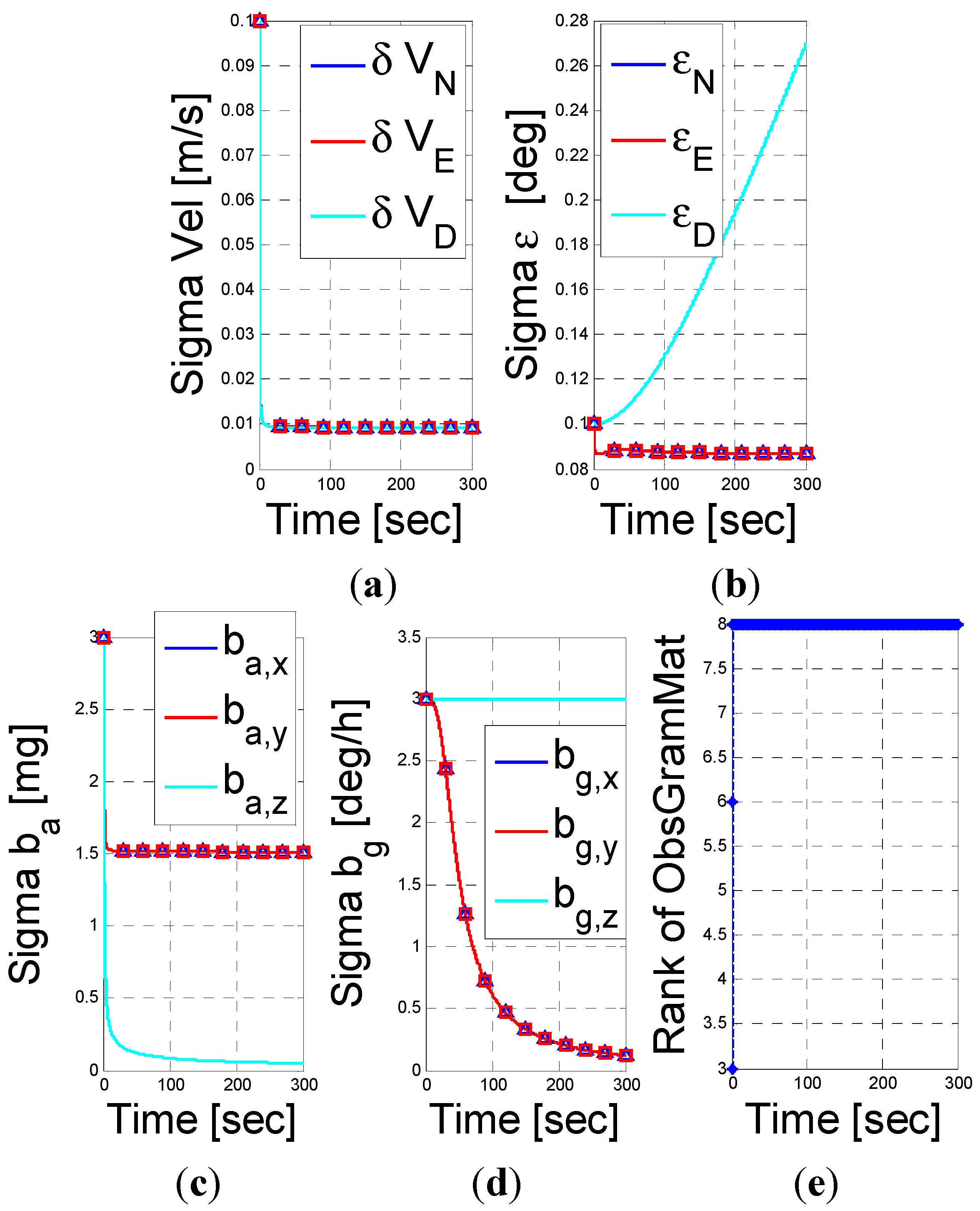
First, in Figure 1, we examined the case of a DVL assisted INS navigation with a stationary vehicle. As mentioned earlier, since the DVL measures the vehicle velocity the position error states are not observable and thus removed of the analysis. Consequently, the system dimension is 12 instead of 15. By Equation (29), the UOS vector is four dimensional and thus we expect the rank of the Gramian matrix to be 8. Observing Figure 1, we immediately see that the rank of the Gramian matrix is 8. Additionally, as indicated by the UOS Equation (29), while the other error parameters converge, the down misalignment angle, z-axis gyro bias, x-y axes accelerometer biases standard deviation does not converge.
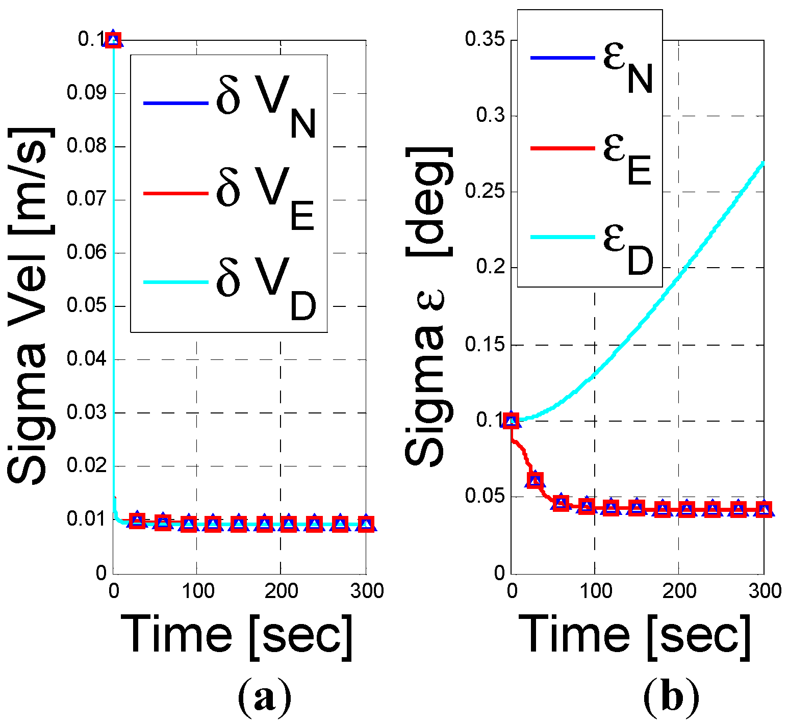
Next, we allow the vehicle to rotate around the z-body (1°/s). The results are shown in Figure 2. As analyzed in Equation (36), the unobservable subspace reduces into a two dimensional vector. As foreseen by our analysis, we observe that only the down misalignment angle and z-axis gyro bias are unobservable. We therefore conclude that the rotation helps to observe the x-y axes accelerometer biases and, as illustrated in Figure 2, the rank of the observability Gramian matrix increases to 10.
Figure 1.
INS/DVL fusion results for a stationery vehicle scenario. (a) velocity error vector; (b) misalignment error; (c) accelerometer residuals; (d) gyro residuals; (e) rank of observbility Gramian matrix.
Figure 1.
INS/DVL fusion results for a stationery vehicle scenario. (a) velocity error vector; (b) misalignment error; (c) accelerometer residuals; (d) gyro residuals; (e) rank of observbility Gramian matrix.

Figure 2.
INS/DVL fusion results for a rotating vehicle scenario. (a) velocity error vector; (b) misalignment error; (c) accelerometer residuals; (d) gyro residuals; (e) rank of observbility Gramian matrix.
Figure 2.
INS/DVL fusion results for a rotating vehicle scenario. (a) velocity error vector; (b) misalignment error; (c) accelerometer residuals; (d) gyro residuals; (e) rank of observbility Gramian matrix.


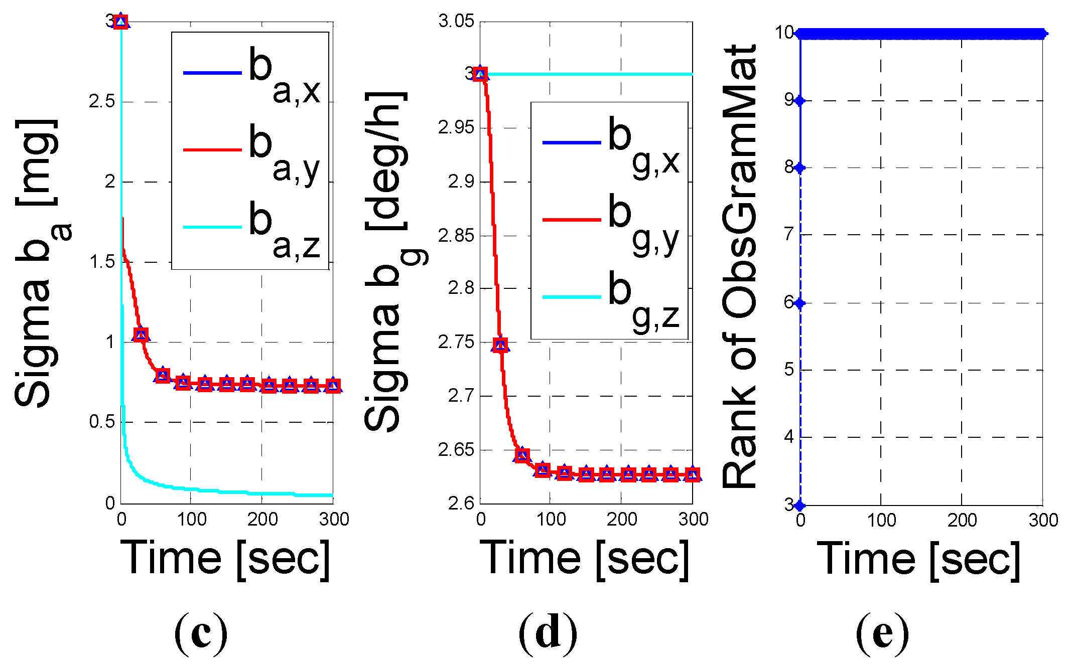
The case of a vehicle travelling with constant speed (10 m/s) and experiences rotation around the z-body (1°/s) is simulated in Figure 3. As given by Equation (39), the unobservable subspace is shown to be of one-dimensional space, where only a linear combination of the down misalignment angle and z-axis gyro bias is unobservable.
Figure 3.
INS/DVL fusion results for a vehicle traveling with constant speed and angular velocity scenario. (a) velocity error vector; (b) misalignment error; (c) accelerometer residuals; (d) gyro residuals; (e) rank of observbility Gramian matrix.
Figure 3.
INS/DVL fusion results for a vehicle traveling with constant speed and angular velocity scenario. (a) velocity error vector; (b) misalignment error; (c) accelerometer residuals; (d) gyro residuals; (e) rank of observbility Gramian matrix.

4.1.2. INS/PS Fusion
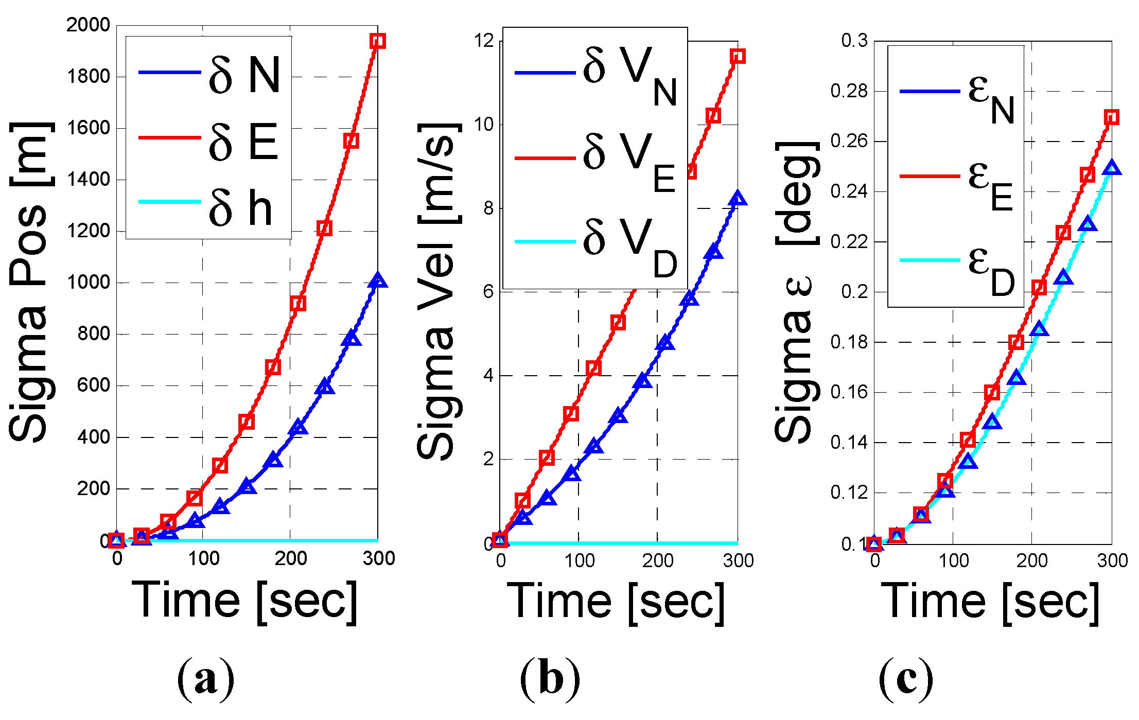
Next, we examine the fusion of the PS assisted INS navigation when the vehicle is stationary. According to the result in Equation (48), only the altitude error, down velocity error, and the z-axis accelerometer bias are observable. The numerical results shown in Figure 4 support this conclusion. In addition, as shown in Figure 4, the rank of the observability Garmin is 3, i.e., an unobservable subspace of rank 12. This result supports our analysis.
Figure 4.
INS/PS fusion results for a stationery vehicle scenario. (a) position error vector; (b) velocity error vector; (c) misalignment error; (d) accelerometer residuals; (e) gyro residuals; (f) rank of observbility Gramian matrix.
Figure 4.
INS/PS fusion results for a stationery vehicle scenario. (a) position error vector; (b) velocity error vector; (c) misalignment error; (d) accelerometer residuals; (e) gyro residuals; (f) rank of observbility Gramian matrix.
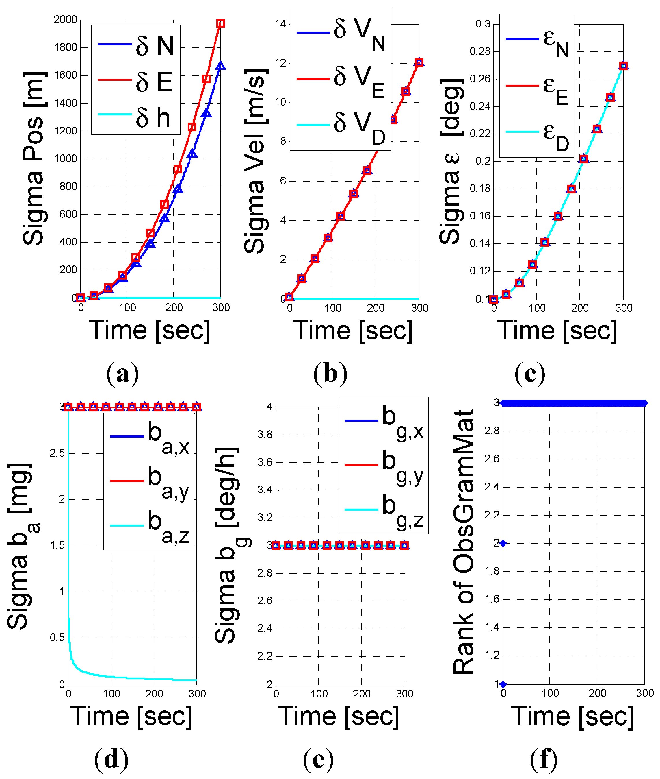
Figure 5.
INS/PS fusion results for a rotating vehicle scenario. (a) position error vector; (b) velocity error vector; (c) misalignment error; (d) accelerometer residuals; (e) gyro residuals; (f) rank of observbility Gramian matrix.
Figure 5.
INS/PS fusion results for a rotating vehicle scenario. (a) position error vector; (b) velocity error vector; (c) misalignment error; (d) accelerometer residuals; (e) gyro residuals; (f) rank of observbility Gramian matrix.

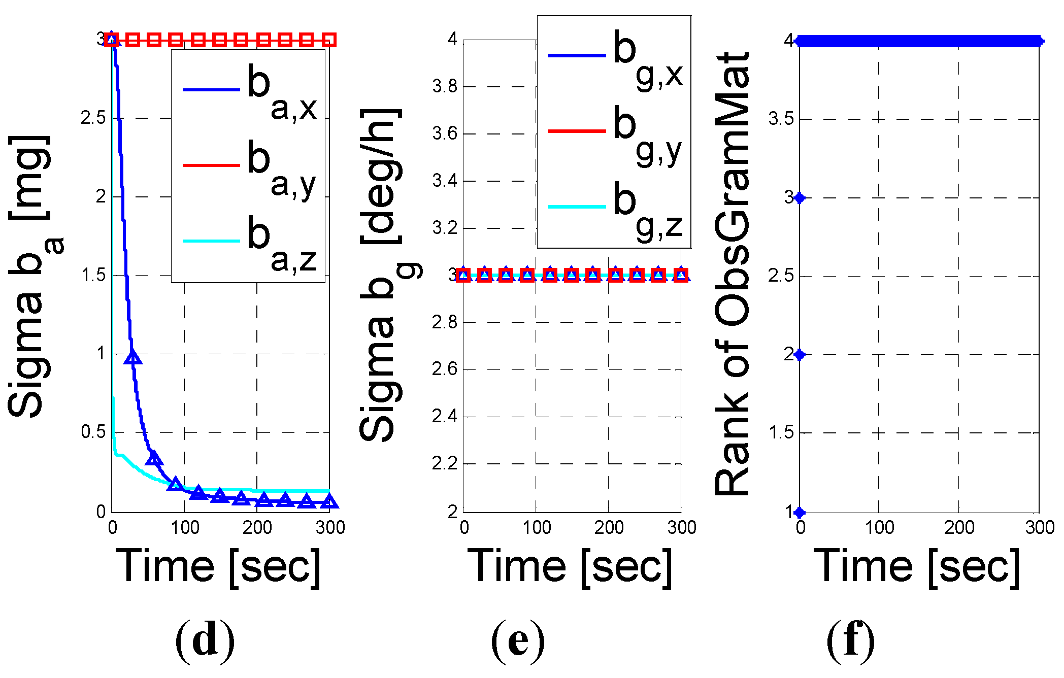
When the vehicle also rotates around the y-body at 1°/s then, by Equation (53), the unobservable subspace reduces into a vector of 11 dimensions. That is, the rotation allows also the estimation of the x-accelerometer bias. This is shown in Figure 5.
Figure 6.
INS/PS fusion results for a vehicle traveling with constant speed and angular velocity scenario. (a) position error vector; (b) velocity error vector; (c) misalignment error; (d) accelerometer residuals; (e) gyro residuals; (f) rank of observbility Gramian matrix.
Figure 6.
INS/PS fusion results for a vehicle traveling with constant speed and angular velocity scenario. (a) position error vector; (b) velocity error vector; (c) misalignment error; (d) accelerometer residuals; (e) gyro residuals; (f) rank of observbility Gramian matrix.
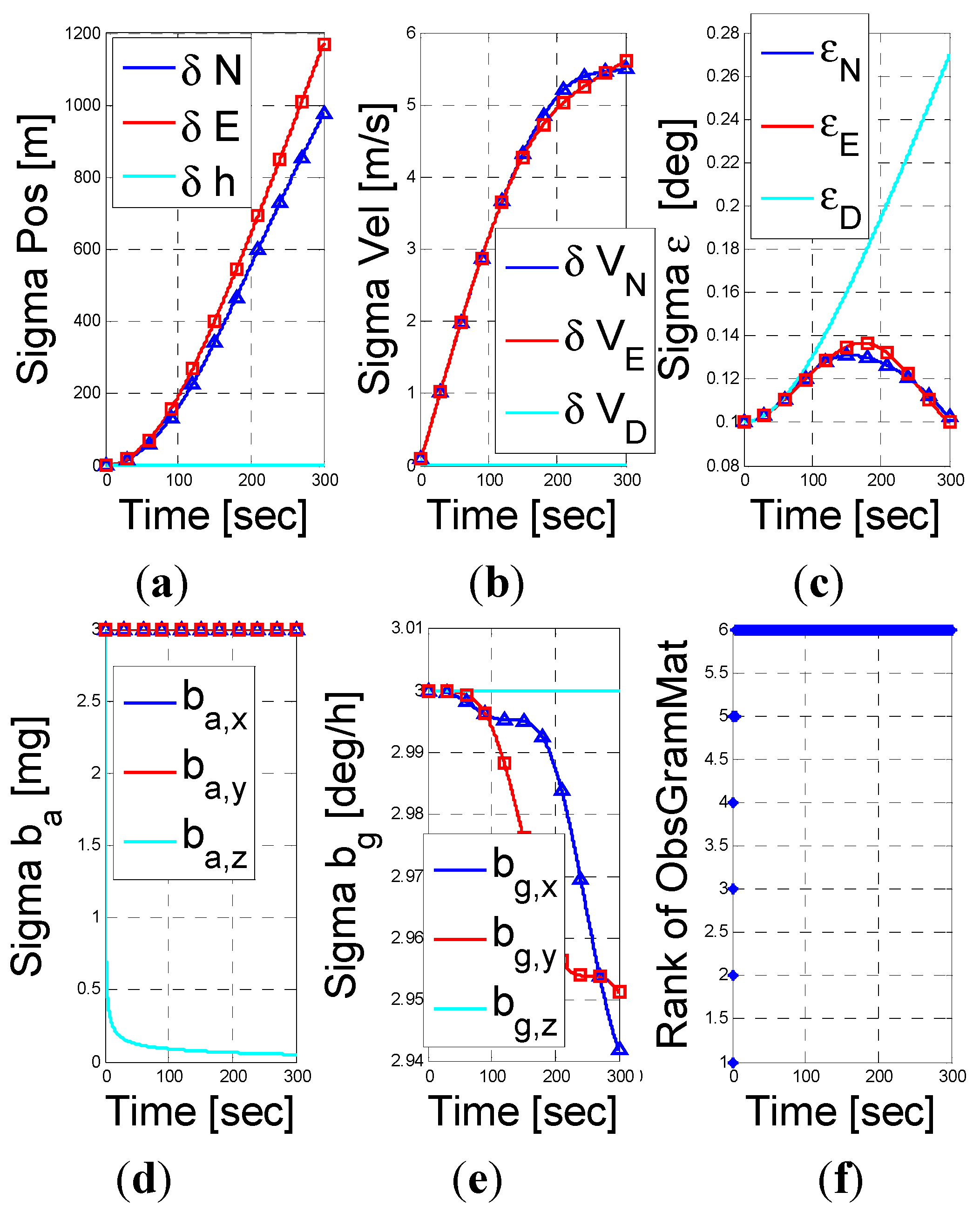
Finally, for the case of a vehicle travelling with constant speed (10 m/s) and experiences rotation around the z-body (1°/s), we predicted in Equation (48) that the unobservable subspace would be a 9 dimensional one. Recall that by Equation (48), without the constant speed the unobservable subspace is 12 dimensional unobservable subspace. That is, the addition of constant speed to the rotation helps reducing the unobservable subspace. As shown in Figure 6, the addition observable states are the x-y axes gyro bias, and the linear combination of the east and north misalignment turned.
4.2. Discussion
Our analysis and simulation for the INS/DVL and INS/PS AUV navigation system showed some interesting results. First, as expected, the observable sub-space becomes larger as maneuvering becomes more complex. That is, perhaps contrary to intuition, AUV path planning should include as much as possible rotating, turning, and motion. In this context, the effect of motion on reducing the unobservable sub-space is the largest. Interestingly, this conclusion applies also for the INS/PS system, which does not include direct measurement of speed.
Second, comparing the results for the INS/DVL and the INS/PS systems, we observe that the observable space for the INS/DVL system has considerably higher rank than that of the INS/PS system. This is an alternative method to observe that a DVL delivers much more information than a PS. Finally, comparing the two navigation systems, we conclude that the effect of maneuvering is considerably higher on the INS/DVL system.
5. Conclusions
In this paper, we focused on the problem of predicting the observable and unobservable error states of the AUV navigation system for several maneuvering types. This is important for understanding the limits of the INS AUV navigation system, as well as to improve path planning for AUVs. Our analysis was based on the observability Gramian approach previously used only for terrestrial applications. We demonstrated our analysis for an INS navigation system assisted by a DVL and by a PS. For each of these systems we analyzed and concluded what would be the unobservable subspace of the navigation error state for different dynamic types. Specifically, we considered the three basic maneuvering types an AUV performs, namely, (1) stationary vehicle (2) stationary vehicle with angular rotation and (3) a vehicle traveling with constant speed and angular rotation. Our results clearly show that the addition of rotation and further linear velocity helps reducing the unobservable subspace, i.e., more error states may be estimated from the measurements. The analytical expressions where verified by numerical simulation. Excact match of the analysis was obtained. That is, the number and identity of the observable and unobservable error states obtained in the simulations match with the analysis for the observability Gramian. Future work will include an analytical observability analysis of the INS/DVL/PS system.
Author Contributions
Itzik Klein has thought of the idea of calculating the unobservable subspace of the DVL/INS and PS/INS systems. From there, the research was made jointly by the two authors.
Conflicts of Interest
The authors declare no conflict of interest.
Nomenclature
| AUV | Autonomous Underwater Vehicles |
| DVL | Doppler Velocity Logger |
| GNSS | Global Navigation Satellite Systems |
| INS | Inertial Navigation Systems |
| PS | Pressure Sensor |
| UOS | Unobservable subspace |
| Φ(t) | State transition matrix |
| δba | Accelerometer bias residuals |
| δbg | Gyro bias residuals |
| δp | Position error vector |
| δv | Velocity error vector |
| δvDVL | DVL velocity measurement residual |
| δx | INS error state vector |
| ε | Misalignment errors |
| ψ | Heading angle |
| θ | Pitch angle |
| ω | Angular velocity vector |
| H(t) | Measurement matrix |
| M | Number of measurements |
| Tb→n | Transformation matrix from body to navigation frame |
| Td→b | Transformation matrix from DVL to body frame |
| a | Acceleration vector |
| f | Specific force vector |
| g | Gravity vector |
| h | Vehicle depth |
| u0 | set of solutions which span the unobservable subspace of the state vector |
| v | Velocity vector |
| (•)n | A vector expressed in the navigation frame |
| (•)b | A vector expressed in the body frame |
| (•)d | A vector expressed in the DVL frame |
| (•)i | A vector expressed in the inertial frame |
References
- Kinsey, J.; Eustice, R.; Whitcomb, L. A survey of underwater vehicle navigation: Recent advances and new challenges. In Proceedings of the 7th IFAC Conference on Maneuvering and Control of Marine Craft (MCMC2006), Lisbon, Portugal, 20–22 September 2006.
- Casari, P.; Zorzi, M. Protocol design issues in underwater acoustic networks. Comput. Commun. 2011, 34, 2013–2025. [Google Scholar] [CrossRef]
- Titterton, D.H.; Weston, J.L. Strapdown Inertial Navigation Technology, 2nd ed.; The Institution of Engineering and Technology: Stevenage, UK, 2004. [Google Scholar]
- Groves, P.D. Principles of GNSS, Inertial and Multisensor Integrated Navigation Systems; Artech House: Norwood, MA, USA, 2008. [Google Scholar]
- Farrell, J.A. Aided Navigation GPS with High Rate Sensors; McGraw-Hill: New York, NY, USA, 2008. [Google Scholar]
- Klein, I.; Filin, S.; Toledo, T. Pseudo-measurements as aiding to INS during GPS outages. NAVIGATION 2010, 57, 25–34. [Google Scholar]
- Vickery, K. Acoustic positioning systems. A practical overview of current systems. In Proceedings of the 1998 IEEE Workshop on the Autonomous Underwater Vehicles, Cambridge, MA, USA, 20–21 August 1998.
- Morgado, M.; Oliveira, P.; Silvestre, C. Tightly coupled ultrashort baseline and inertial navigation system for underwater vehicles: an experimental validation. J. Field Robot. 2013, 30, 142–170. [Google Scholar] [CrossRef]
- Barkby, S.; Williams, S.; Pizarro, O.; Jakuba, M. Incorporating prior maps with bathymetric distributed particle SLAM for improved AUV navigation and mapping. In Proceedings of the OCEANS 2009, MTS/IEEE Biloxi—Marine Technology for Our Future: Global and Local Challenges, Biloxi, MS, USA, 26–29 October 2009.
- Morice, C.; Veres, S.; McPhail, S. Terrain referencing for autonomous navigation of underwater vehicles. In Proceedings of the IEEE Oceans 2009-Europe, Bremen, Germany, 11–14 May 2009.
- Brokloff, N. Matrix algorithm for Doppler sonar navigation. In Proceedings of Oceans 94 OSATES: Oceans engineering for today’s technology and tomorrow’s preservation, Brest, France, 13–16 September 1994; pp. 378–383.
- Jalving, B.; Gade, K.; Svartveit, K.; Willumsen, A.; Sørhagen, R. DVL velocity aiding in the HUGIN 1000 integrated inertial navigation system. Model. Identif. Control 2004, 25, 223–235. [Google Scholar] [CrossRef]
- Troni, G.; Whitecomb, L.L. Experimental evaluation of a MEMS inertial measurements unit for Doppler navigation of underwater vehicles. In Proceedings of the Oceans 2012, Hampton Roads, VA, USA, 14–19 October 2012.
- Miller, P.A.; Farrell, J.A.; Zhao, Y.; Djapic, V. Autonomous underwater vehicle navigation. IEEE J. Ocean. Eng. 2010, 35, 663–678. [Google Scholar] [CrossRef]
- Lee, P.; Jun, B. Pseudo long base line navigation algorithm for underwater vehicles with inertial sensors and two acoustic range measurement. IEEE J. Ocean Eng. 2007, 34, 416–425. [Google Scholar] [CrossRef]
- Rhee, I.; Abdel-Hafez, M.F.; Speyer, J.L. Observability of an Integrated GPS/INS during Maneuvers. IEEE Trans. Aerosp. Electron. Syst. 2004, 40, 526–535. [Google Scholar]
- Hegrenaes, O.; Berglund, E. Doppler water-track aided inertial navigation for autonomous underwater vehicle. In Proceedings of the IEEE Oceans Conference and Exhibition, Bremen, Germany, 11–14 May 2009.
- Geng, Y.; Martins, R.; Sousa, J. Accuracy Analysis of DVL/IMU/Magnetometer Integrated Navigation System using Different IMUs in AUV. In Proceedings of the 8th IEEE International Conference on Control and Automation, Xiamen, China, 9–11 June 2010.
- Maybeck, P.S. Stochastic Models, Estimation and Control; Academic Press: New York, NY, USA, 1982. [Google Scholar]
- Ham, F.; Brown, R. Observability, eigenvalues, and Kalman filtering. IEEE Trans. Aerosp. Electron. Syst. 1983, 19, 269–273. [Google Scholar] [CrossRef]
- Ramanandan, A.; Chen, A.; Farrell, J.A. Inertial Navigation Aiding by Stationary Updates. IEEE Trans. Intell. Transp. Syst. 2011, 13, 235–248. [Google Scholar] [CrossRef]
- Rottman, Y.; Klein, I.; Filin, S. Analytical Observability Analysis of INS with Vehicle Constraints. NAVIG. J. Inst. Navig. 2014, 61, 227–236. [Google Scholar] [CrossRef]
- Klein, I.; Bar-Shalom, Y.; Rusnak, I. Observability analysis for tracking of coordinated turn maneuvers. In Proceedings of the IEEE 28-th Convention of Electrical and Electronics Engineers, Eilat, Israel, 3–5 December 2014.
- Goshen-Meskin, D.; Bar-Itzhack, I.Y. Observability analysis of piecewise constant systems—Part I: Theory. IEEE Trans. Aerosp. Electron. Syst. 1992, 28, 1056–1067. [Google Scholar] [CrossRef]
- Goshen-Meskin, D.; Bar-Itzhack, I.Y. Observability analysis of piecewise constant systems—Part II: Application to inertial navigation in-flight alignment. IEEE Trans. Aerosp. Electron. Syst. 1992, 28, 1068–1075. [Google Scholar] [CrossRef]
- Hong, S.; Lee, M.H.; Chun, H.-H.; Kwon, S.-H.; Speyer, J.L. Observability of error states in GPS/INS integration. IEEE Trans. Veh. Technol. 2005, 54, 731–743. [Google Scholar] [CrossRef]
- Hong, S.; Lee, M.H.; Chun, H.-H.; Kwon, S.-H.; Speyer, J.L. Experimental study on the estimation of lever arm in GPS/INS. IEEE Trans. Veh. Technol. 2006, 55, 431–448. [Google Scholar] [CrossRef]
- Tang, Y.; Wu, Y.; Wu, M.; Wu, W.; Hu, X.; Shen, L. INS/GPS Integration: Global Observability Analysis. IEEE Trans. Veh. Technol. 2009, 58, 1129–1142. [Google Scholar] [CrossRef]
© 2015 by the authors; licensee MDPI, Basel, Switzerland. This article is an open access article distributed under the terms and conditions of the Creative Commons Attribution license (http://creativecommons.org/licenses/by/4.0/).
Share and Cite
MDPI and ACS Style
Klein, I.; Diamant, R. Observability Analysis of DVL/PS Aided INS for a Maneuvering AUV. Sensors 2015, 15, 26818-26837. https://doi.org/10.3390/s151026818
AMA Style
Klein I, Diamant R. Observability Analysis of DVL/PS Aided INS for a Maneuvering AUV. Sensors. 2015; 15(10):26818-26837. https://doi.org/10.3390/s151026818
Chicago/Turabian StyleKlein, Itzik, and Roee Diamant. 2015. "Observability Analysis of DVL/PS Aided INS for a Maneuvering AUV" Sensors 15, no. 10: 26818-26837. https://doi.org/10.3390/s151026818