A Novel Diagnosis Method for a Hall Plates-Based Rotary Encoder with a Magnetic Concentrator


Abstract
: In the last few years, rotary encoders based on two-dimensional complementary metal oxide semiconductors (CMOS) Hall plates with a magnetic concentrator have been developed to measure contactless absolute angle. There are various error factors influencing the measuring accuracy, which are difficult to locate after the assembly of encoder. In this paper, a model-based rapid diagnosis method is presented. Based on an analysis of the error mechanism, an error model is built to compare minimum residual angle error and to quantify the error factors. Additionally, a modified particle swarm optimization (PSO) algorithm is used to reduce the calculated amount. The simulation and experimental results show that this diagnosis method is feasible to quantify the causes of the error and to reduce iteration significantly.1. Introduction
Magnetic position sensors mainly include two types. One uses a rotating permanent magnet, while others adopt a steel target wheel with teeth and slots that modulate the flux from a stationary magnet. These flux modulations can be read by semiconductors (Hall sensors or magneto resistors) [1–3]. Hall sensors are widely used to sense the rotation of moving mechanical components, they have the advantages of lower cost and higher reliability in harsh environments. Moreover, a Hall sensor-based rotary encoder has a linear response to magnetic flux density, while not having electrical hysteresis [4,5]. Hall plates placed on the periphery of a rotating magnet can be used to measure 360° absolute angle, but rotary encoders based on this principle are very sensitive to the misalignment between the sensor and magnet [2,6].
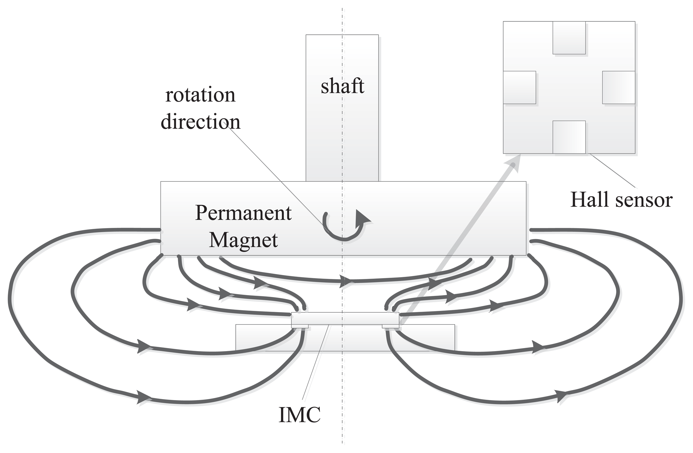
To reduce the influence of the misalignment and to improve the performance, a magnetic angular sensor using Hall plates placed on the periphery of a CMOS Hall application specific integrated circuit (ASIC), which is formed an integrated magnetic concentrator (IMC), was invented [7,8]. An illustration of its layout and cross-section is shown in Figure 1. The magnetic field is parallel to a Hall sensor converted into a perpendicular field, while it passes through the IMC. The angle can be calculated by measuring the voltage of the Hall plate, which is vertically placed on the periphery of the IMC.
Different techniques, such as offset compensation, signal conditioning, spinning current Hall probe and phase compensation, have also been used to improve the performance of the rotary encoder [9–13]. Additionally, front-end calibration is performed during the final test of the sensor component, which is used to compensate for the error factors, including offset, phase and mismatch. After the assembly of the rotary encoder, the overall errors due to off-axis, tilting and magnetic error are compensated through back-end calibration.
When factors, including stray magnetic fields and the accuracy of the mechanical alignment, exceed the limit, the systematic error will get out of control. Mechanical alignment and other back-end calibration errors can result in additional offset, phase shift, amplitude change and non-linearity, which will reduce the precision of the encoder [14,15].
Using the traditional measurement methods, it is not always a simple affair to quantify each error factor after the assembly of the encoder. Model-based analytical calculation provides a way for magnetic field simulation and error analysis [15–17]. However, it is difficult to find a theoretical or experimental formula, that considers all of the factors. Yet, it still has some troubles, such as tediously long computation.
This study investigated the effects of different factors, including offset, gain mismatch, phase deviation, non-Linearity, voltage fluctuation, calculation error and other immeasurable factors. Based on the analysis of the error mechanism, an error model is built to compare the minimum residual angle error and the quantify the error factors. Moreover, a modified PSO algorithm is applied to accelerate the calculation process.
The main contribution of this paper is bridging front-end calibration and back-end calibration using the model-based method. Using this method, error sources can be quantified by parameters and front-end calibration can be performed after the assembly of the encoder. Using these parameters, the back-end compensation parameters can be changed from the discontinuity point to a continuity curve, and the small changes during the manufacturing process also can be monitored.
2. Error Mechanism
2.1. Analysis of the Error Sources
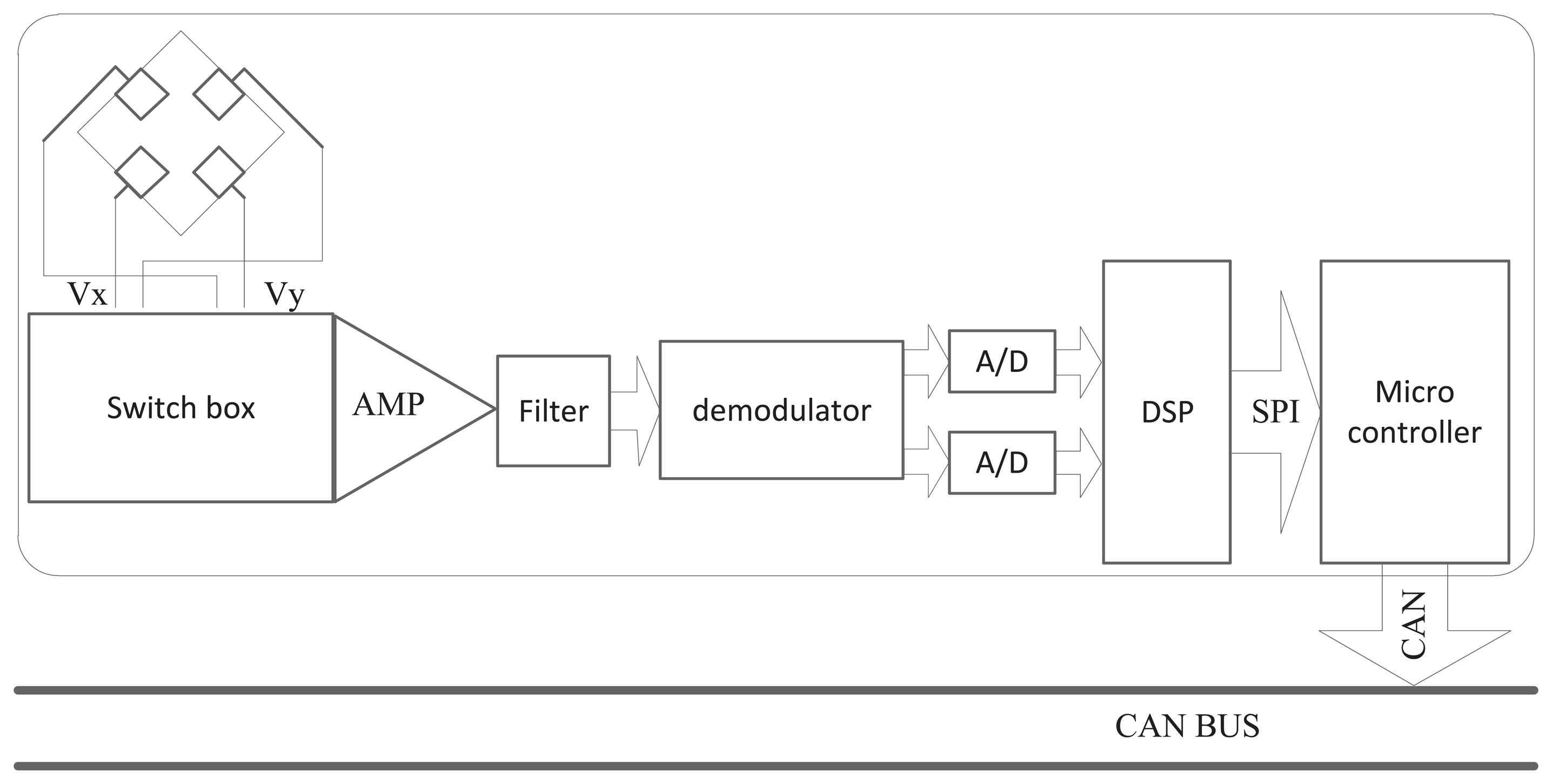
The rotary encoder-based on Hall plates with a magnetic concentrator is made up of several different parts, including a switch box, a filter and amplifying circuit, a synchronous demodulator, digital signal processing (DSP), and so on. The constitution of the rotary encoder is shown in Figure 2. Both Vx and Vy are multiplexed via an adapted clock sequence for the spinning current switch boxes. After the processing of the filter, the sampling and holding are used for the demodulation. The DSP converts the voltage signal, which is amplified from the voltage on Hall plates into the angle signal. Then, the micro-controller acquires the real-time angle signal, through the serial peripheral interface (SPI). The encoded rotation angle is finally sent out by the controller area network (CAN) after compensating.
The performance of the rotary encoder depends on several factors, such as the offset, misalignment, gain mismatch, non-linearities, noise, quantization error, calculation error, and so on [12–14]. Special technology is necessary to limit the offset and ensure signal consistency. Just as with the signal processing technology shown in Figure 2, both axes are multiplexed via an adapted clock sequence for the spinning current switch boxes. Moreover, quadrature spinning and a chopper stabilized amplifier are effective ways to limit the offset. Of course, the influence of these cannot be eliminated completely [9,10].
Misalignment refers to two perpendicular Hall plates not being aligned and the magnetic field not being aligned with the Hall plates. However, in fact, the misalignment does not come from the CMOS process, because the machining precision of CMOS is up to 0.1μm. The source of misalignment is the IMC, which is attached on top of the die at the end of the process line: this IMC is shifted against the die, due to the placement tolerances. Moreover, the shape of the IMC should ideally be a flat disk, but in reality, its perimeter has a poor quality, due to process reasons (rough surface with small mouse-bites, etc.). This leads to the orthogonal errors of both axes [18].
The process imperfections, like mask misalignment and etching tolerances, lead to mismatch in sensitivity and orthogonality between measurement axes [11,19].
Non-linearities (NL) occur with the variations of the magnetic field, which contributes to the angular measurement distortions. The magnetic NL is about 0.5 mT for a magnetic field up to 80 mT. Absolute non-linearity (ANL) is defined as the deviation from the best linearities with a unitary slope. For every sample, an ANL of the second harmonic is observed; the sources of this type of ANL will gain the mismatch and non-orthogonality of the sensor axes [9,12,14].
Analogous to digital sampling, which also brings error, the influence can be reduced through improving the sampling accuracy. Meanwhile, the calculation of the arctangent is the possible error source. The CORDIC algorithm is a general method to calculate the arctangent, whose influence is foreseeable.
Some factors, including the mechanical deviation, are easy to understand, while others are not obvious. Due to the measurement limitations, their influences cannot be quantized, but their influences can still be expected to follow the formula given below [18].
- –
α is the angle measured by the rotary encoder, while α is the standard angle.
- –
Ax and Ay are the magnetic sensitivity along the x- and y-axes, respectively;
- –
Vx and Vy are the offsets of the x- and y-axes, respectively.
- –
β is the orthogonality correction angle (phase error).
Meanwhile, the influences of temperature, abrasion and the errors caused by other devices also follow the general error mechanism, but showing different characteristics in specific conditions.
2.2. Influence of Error Factors
2.2.1. Offset Error
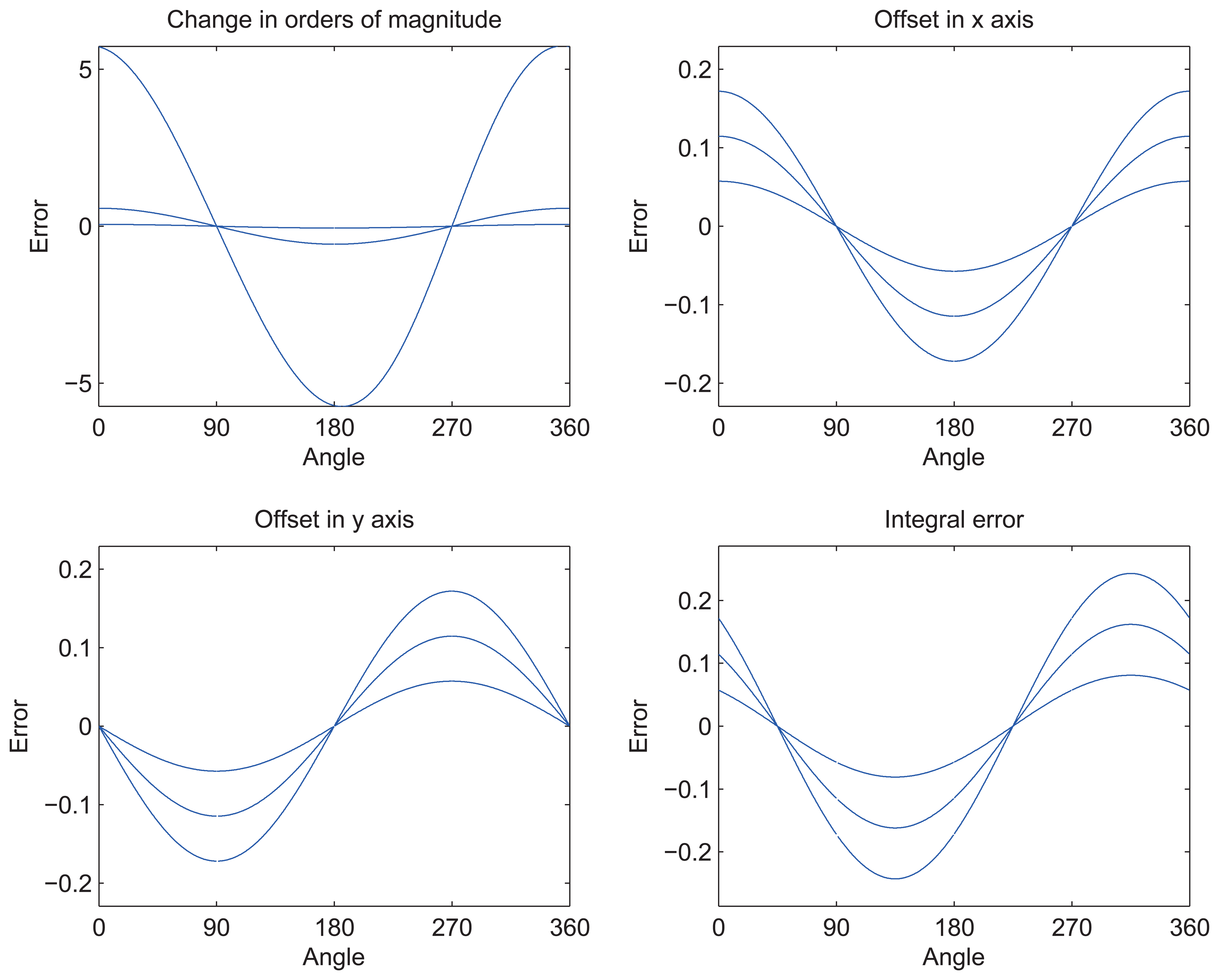
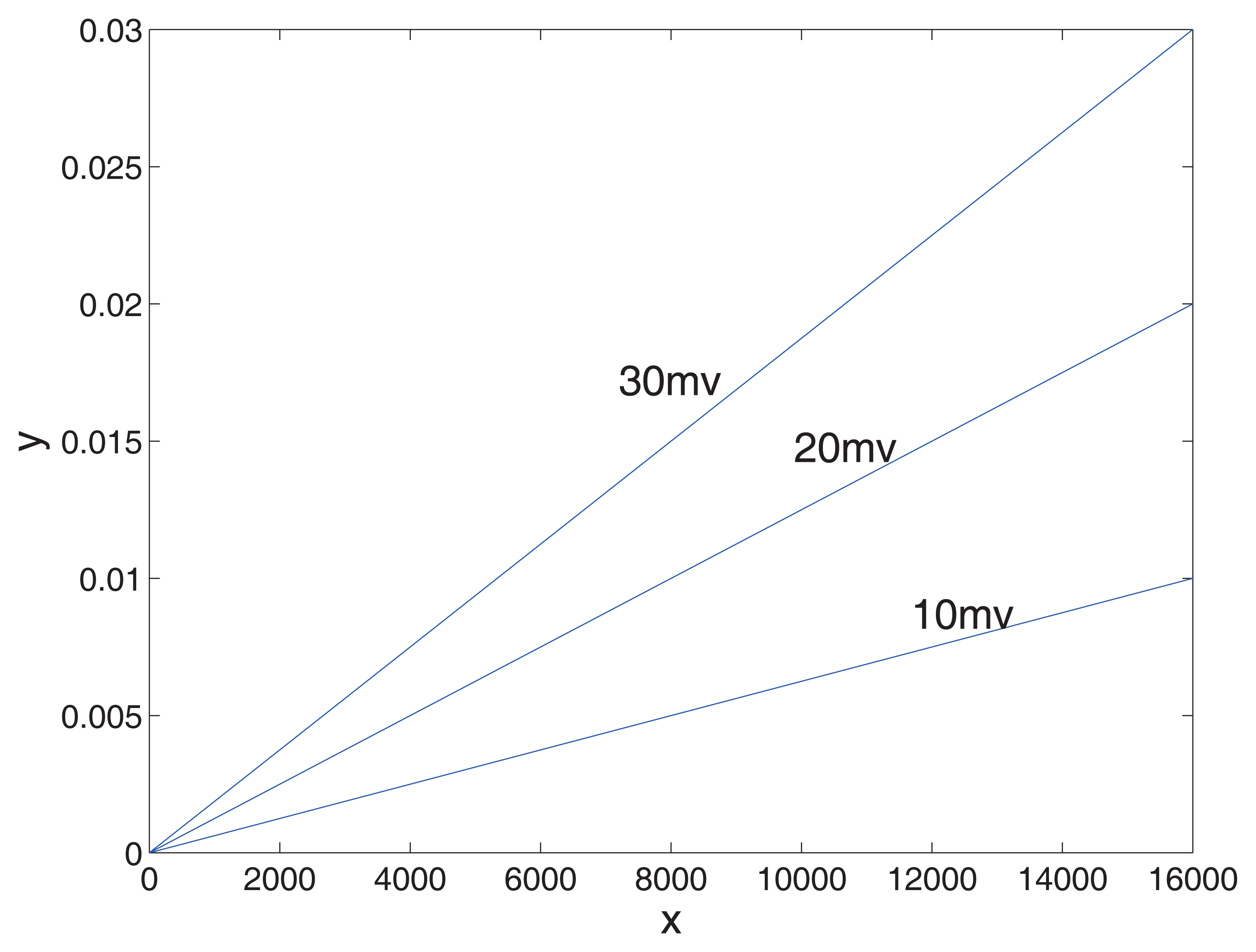
Offset voltage is often small and related to temperature. The relative angle error curve in different offset conditions is shown in Figure 3.
Subgraph 1 shows the error curves when the offset of the axis changes in orders of magnitude. Subgraphs 2 and 3 show the error curves when the offset changes in the x-axis and y-axis (offset of 1 mv, 2 mv and 3 mv). Integral error shows the trend of error when the offset changes in both the x- and y-axes.
As the figure shows, offset and error change in the same order of magnitude. Degree is the unit of angle error, while volt is the unit of the corresponding offset.
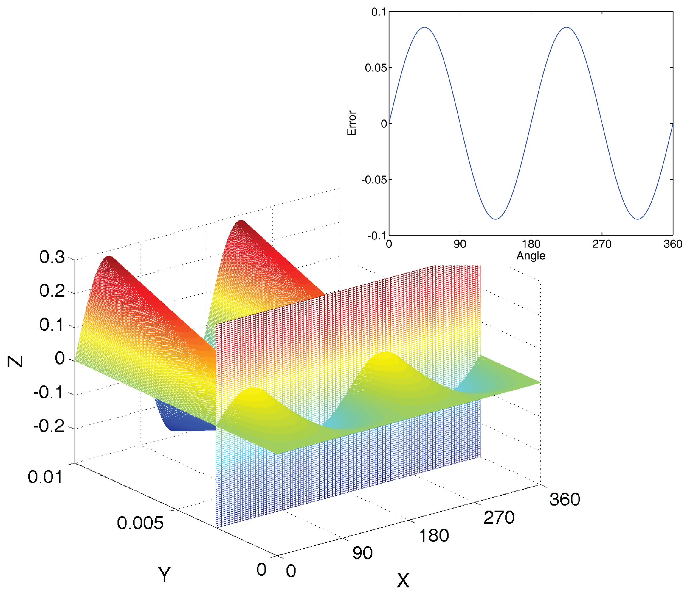
2.2.2. Gain Mismatch
Commonly, the mismatch exists in a unit of one in a thousand. After gain compensation using the previously measured magnetic values, the absolute error can experimental be reduced by half.
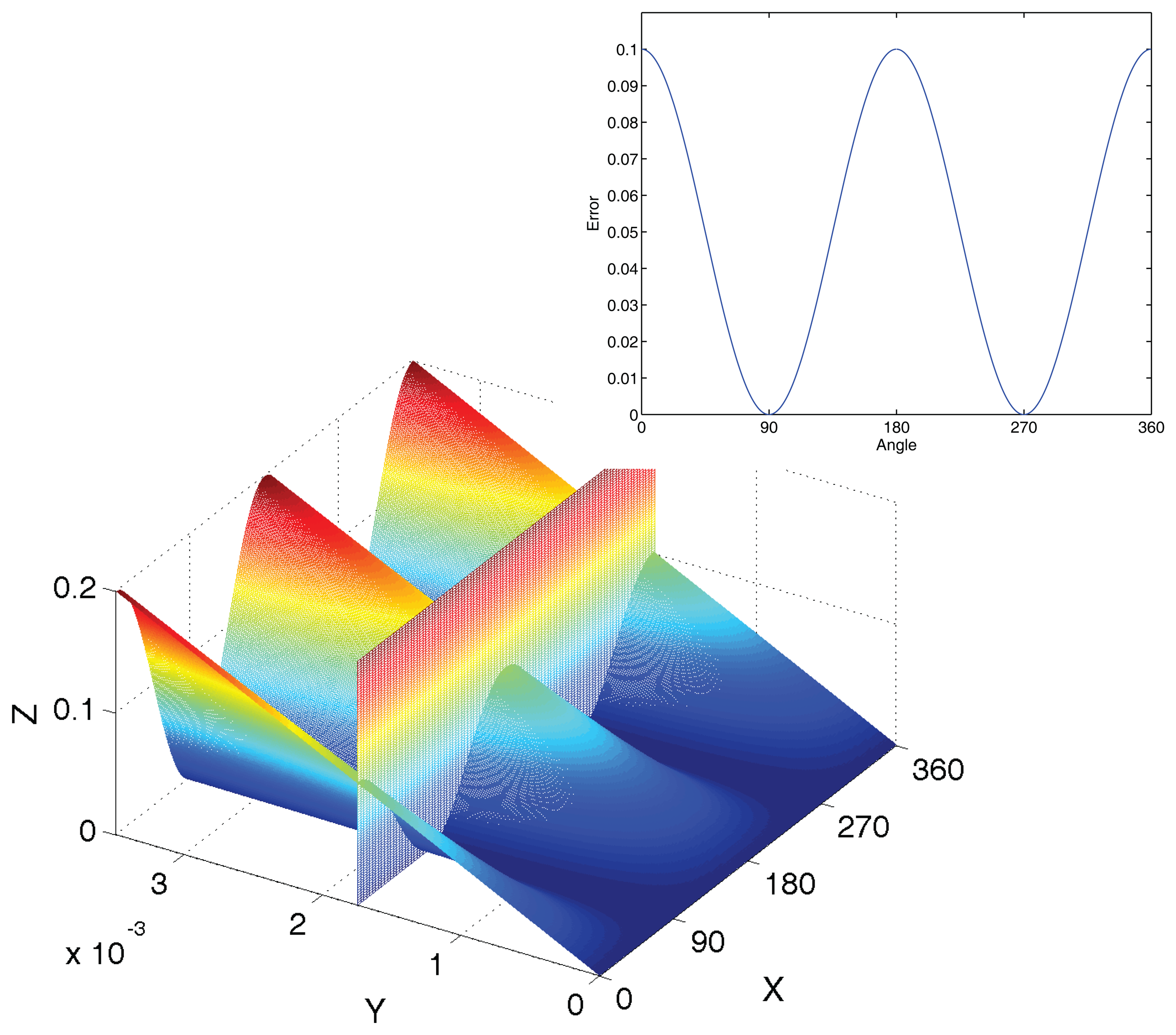
As shown in Figure 4, the error caused by gain mismatch presents two cycle changes in 360°, and it is directly proportional to the percentage of mismatch.
2.2.3. Phase Error
Misalignment and hysteresis appear in the form of the phase error, a curve of which is shown in Figure 5. Usually, phase deviation caused by hysteresis is below 0.05°, while it can be up to 0.1° or even above, considering misalignment and other effects.
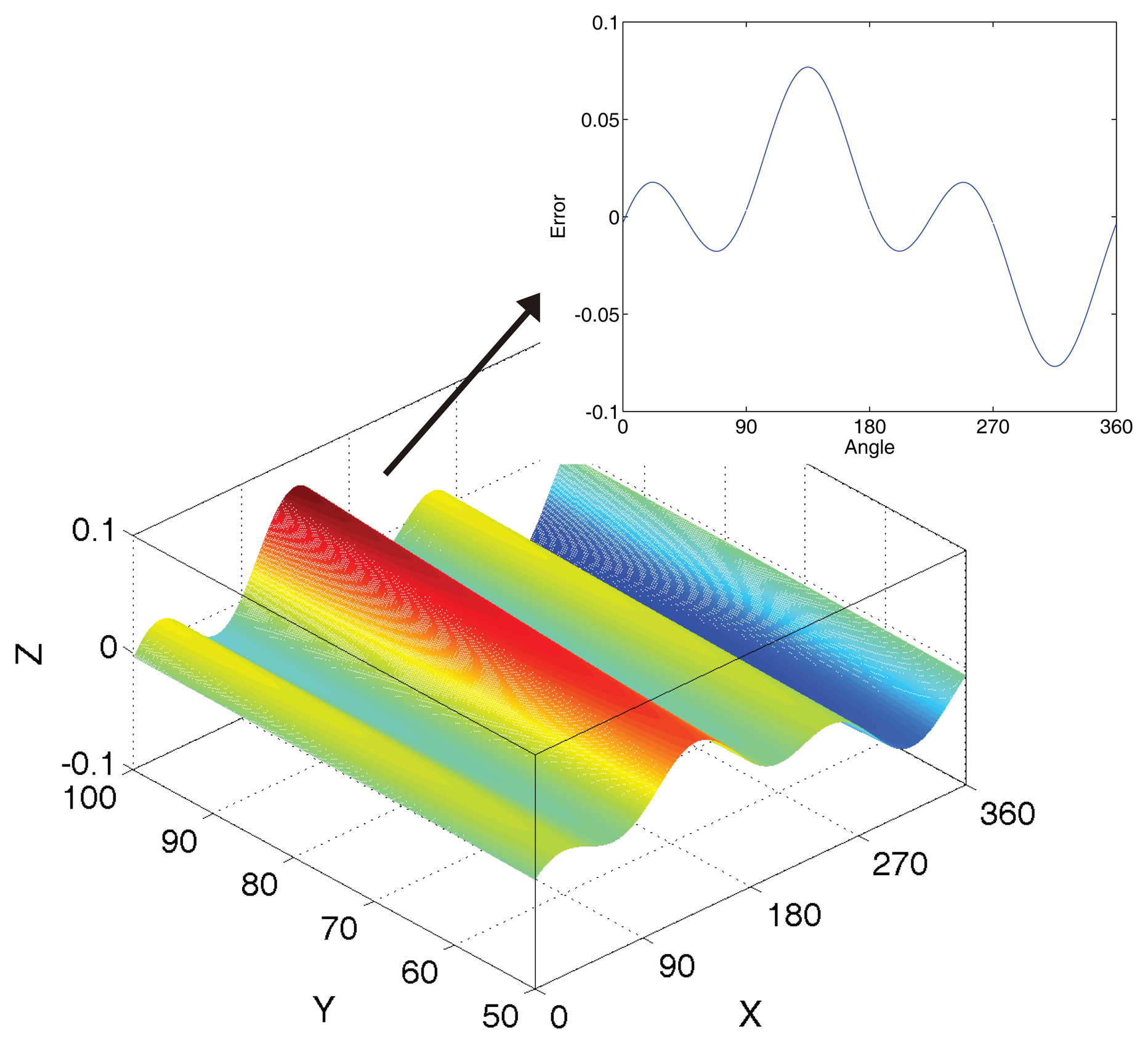
2.2.4. Non-Linearity
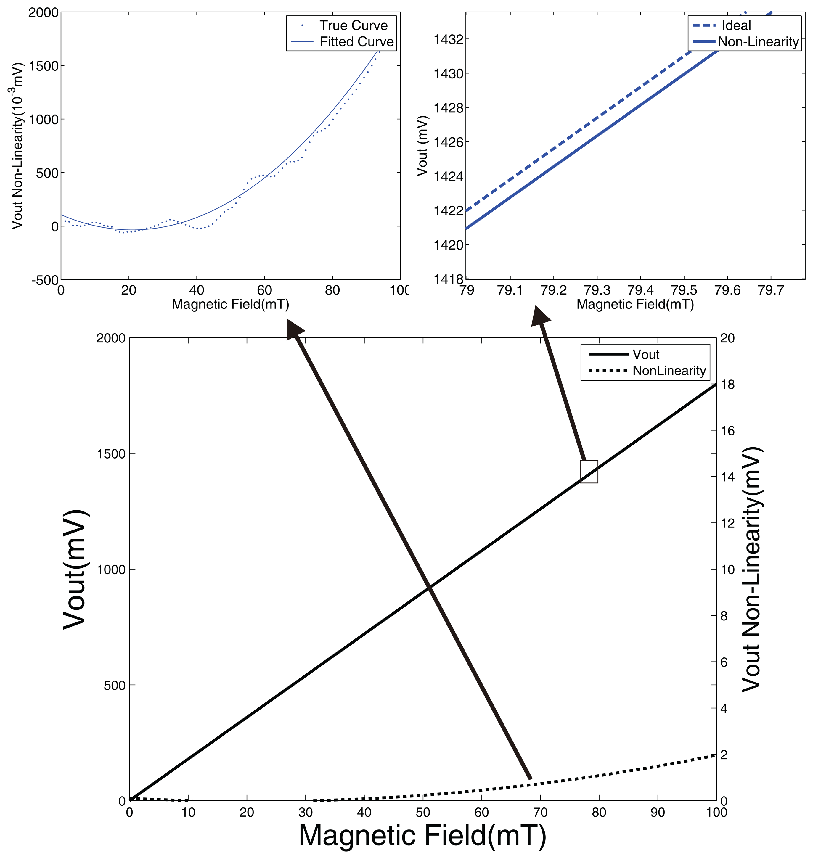
Normally, the non-linearity of the signal is negligible. In the situation of magnetic saturation (the applied field on the IMC location is greater than the saturation value) or low magnetic field, the non-linearity is not ignorable. The relationship between magnetic field intensity and output voltage is shown in Figure 6. The election and installation of a permanent magnetic material is essential for avoiding non-linearity.
The polynomial parameters of the non-linearity curve are concerned with the properties and the size of permanent magnetic materials. A formula of polynomial fitting is quadratic polynomial, as follows.
when K1, K2, K3 are polynomial parameters of non-linear equations from magnetic fields. magx is the maximum magnetic field intensity measured in the Hall plate. Of course, the analysis method of the magnetic field is also a way to get a fitting curve [16]. The angle error curve of non-linearity is shown in Figure 7.
2.2.5. Voltage Fluctuation
Voltage fluctuation is inevitable. The volatility of the reference voltage directly leads to the sampling errors. Error ω related to the quantization noise of the ADC can be expressed as the following formula.
ΔD is the reference value and m is the sampling accuracy of the ADC. In 14-bit accuracy, quantitative values of sampling voltage x are from zero to 16,383. The sampling error is caused by voltage fluctuation, as presented as Figure 8.
The error increases with the voltage amplitude. Essentially, the voltage fluctuation is the value of the reference voltage offset from the ideal. Usually, this inconsistency is caused by the instability of external input voltage [20,21].
2.2.6. Calculation Error
Calculation of the arctangent is also a source of error. The table-lookup algorithm has the features of being fast and simple. However, it needs a large storage space, and computing precision cannot be well guaranteed [22].
Another effective calculation method is the CORDIC algorithm. The CORDIC algorithm is an iterative technique to compute several trigonometric and hyperbolic functions by using additions and shifts [23,24].
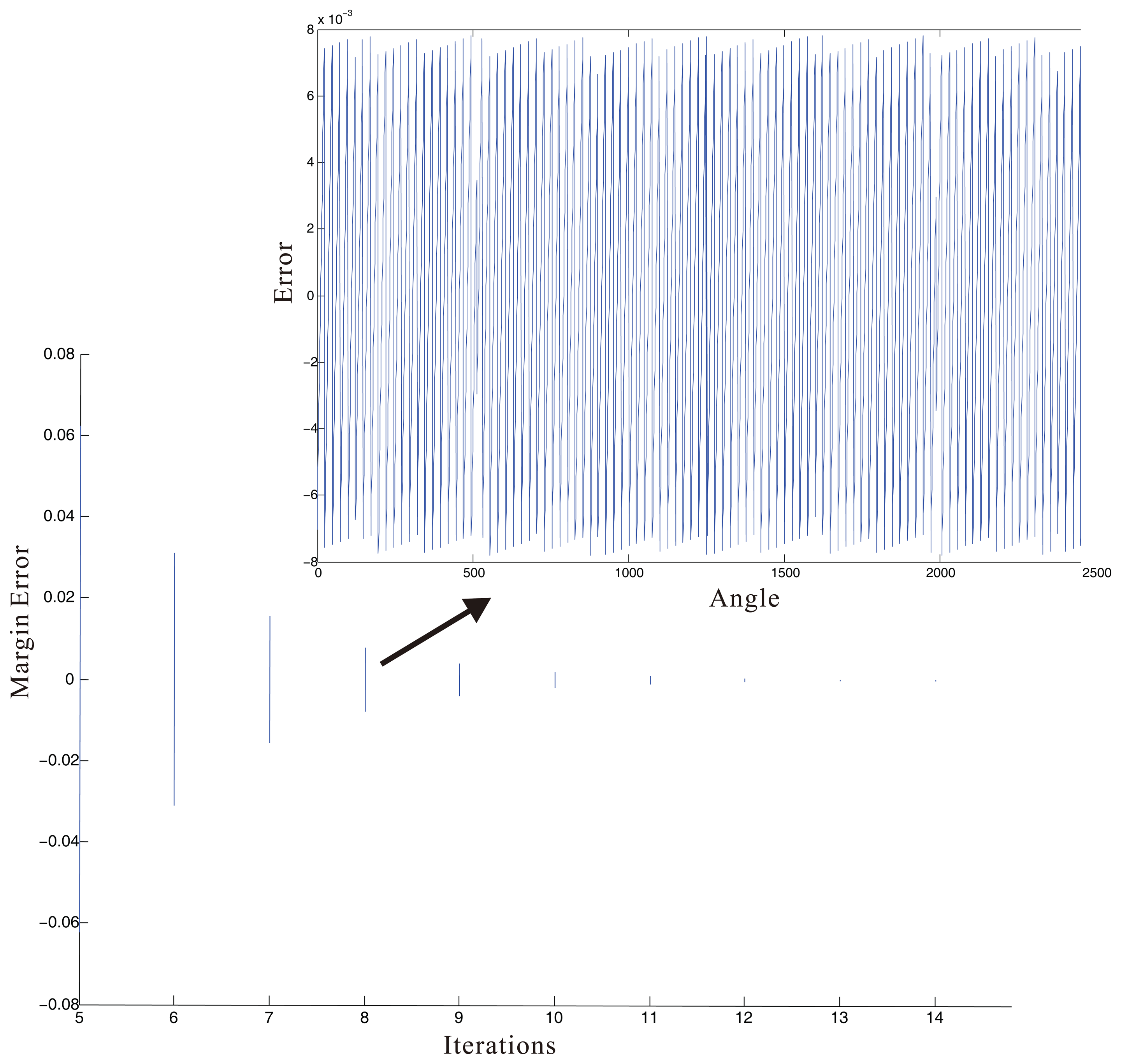
Errors in the CORDIC algorithm are mainly of two types: (1) the angle approximation error, which originates from the quantization of the rotation angle represented by a linear combination of finite numbers of elementary angles; (2) the finite word length of the data path resulting in the rounding/truncation of the output, which increases cumulatively through the successive iterations of micro-rotations [25]. The calculation error of a general pipelined CORDIC architecture is shown in Figure 9. Modified CORDIC algorithms can reduce the iteration time, but the changes of the error margin are similar.
2.3. Modeling the Errors
The influence of factors can be revealed using a single factor to calculate the error. The influence of the single factors, which approaches, reality, is presented in Table 1.
Obviously, the magnitude of error is mainly affected by the offset, gain mismatch, phase deviation, non-linearity and voltage fluctuation. Meanwhile, quantization, calculation and other factors have an impact on the fluctuation range of the error. The influences of quantization and calculation are foreseeable. Although the influences of other factors are immeasurable, they have only a limited impact. With comprehensive consideration of the Equations (1) and (2), the model to diagnose the error can be described as follows [17,26].
- –
Pnk is the value of α′ −α when angle numbers are n and the parameter number is k.
- –
Vyk, Ayk, Vxk, Axk, βk is parameters value of number k.
- –
αn is α with the number of n in the scope of the whole cycle.
F (αn) is defined as the formula below.
Now, we have a clear understanding of error factors. Additionally, there are a couple of parameters values to present the error of the encoder measurement results. Using these parameters, the error parameters of key factors can be quantified; where we still see the problem that a single error factor is immeasurable and there exist interactions among different factors; which leads us to introduce the model-based diagnosis method.
It works like this: For all of the variables, a couple of values are assumed within the possible range, and then the calculating of the results of these assumed values are compared with the actual results. By comparing the minimum residual angle error, the variables most consistent with the practice ones can be obtained. In the below formula, Rk is the minimum residual angle error of a couple of values in six dimensions.
The range of fluctuation is used to choose the optimal solution, as there might be more than one result.
The fluctuation can be scaled by:
- –
ΔE is the fluctuation range of α′ −α.
- –
σrms is the quantization error.
- –
ω is the error caused by the voltage fluctuation.
- –
δ is immeasurable error.
If the fluctuation goes beyond the range, this set of solutions should be removed.
3. Structure of the Diagnostic System
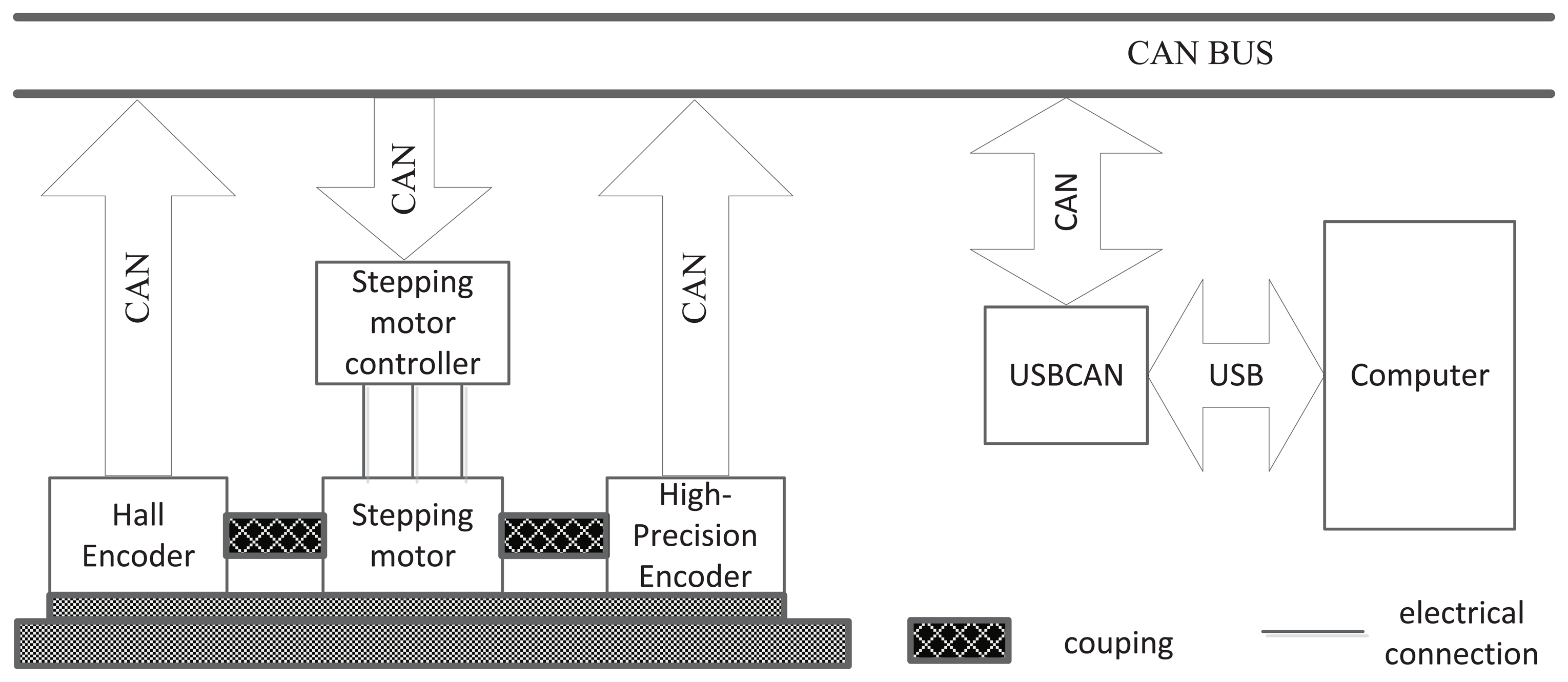
To realize the diagnostics, a diagnostic system is presented, the structure of which is shown in Figure 10.
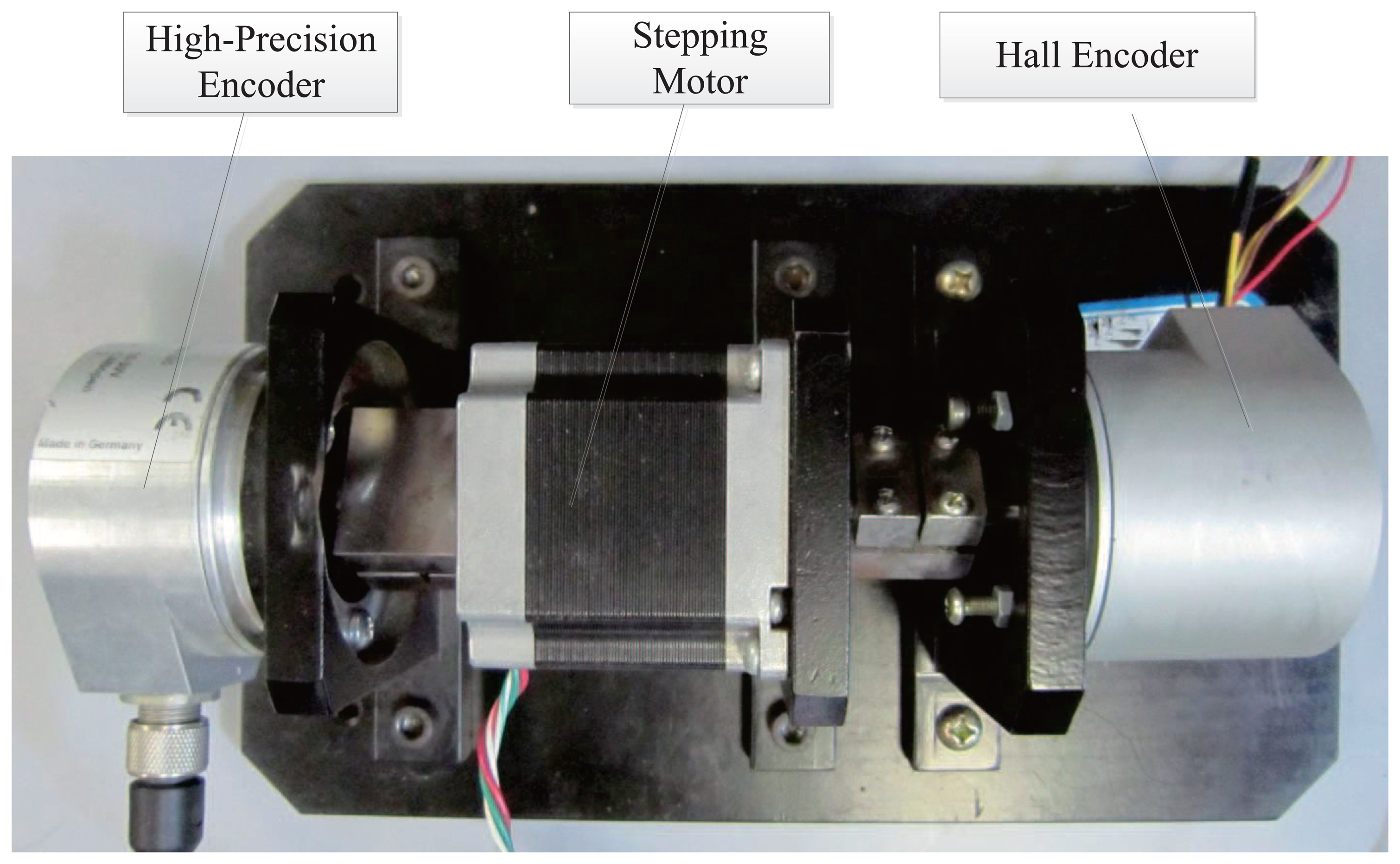
In this system, a high-precision encoder and a Hall encoder are used to measure the angle of a shaft while a computer controls the whole system. A USBCAN device is used to work as a router between CAN and Universal Serial Bus (USB). The computer-controlled diagnostics system works under a prescribed sequence, through receiving data and sending commands. Firstly, the stepping motor controller drives the shaft to special angle by receiving command from computer. After shaft stopped in a special angle; the computer receives the measurement results from the high-precision encoder and the Hall encoder. Through comparing two measurement results, the error of a specific angle is obtained. In the same way, the error of the whole circle can be obtained. A real picture of diagnostic platform is shown in Figure 11.
4. Rapid Diagnosis Method Using PSO
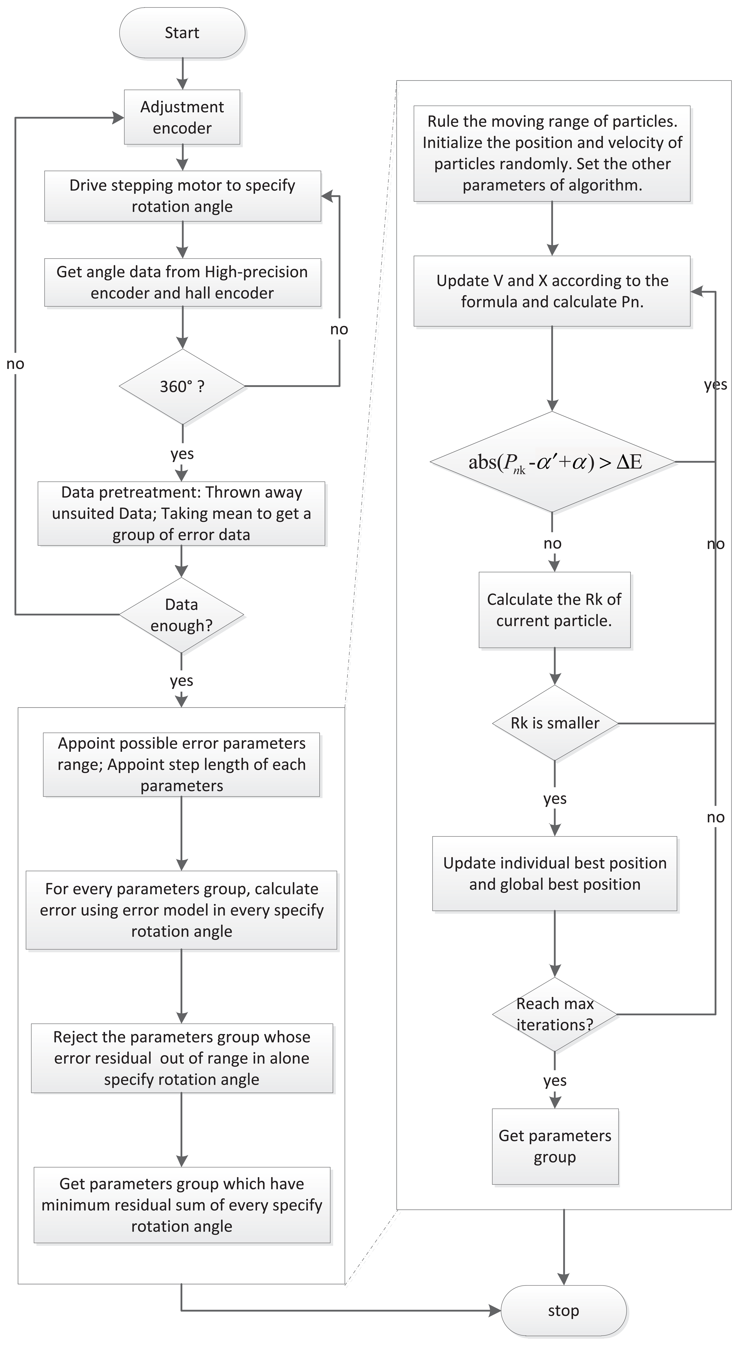
4.1. The Process of the Rapid Diagnosis Method
Through a comparison with a high-precision standard rotary encoder, the Hall encoder's error in the whole circle can be obtained. Pretreatment and preliminary judgment can be used to reject manifest errors and provide reliable data. After that, the error factors are quantified through comparing the minimum residual angle error. Using an ordinary method, it is necessary to make a calculation for every step in the range of each parameter.
The PSO algorithm has supplied an effective method for the fitting of continuous non-linear functions [27]. So as to improve efficiency, the PSO algorithm is applied to compare the minimum residual angle error and to quantify the error factors. However, there are two problems: the minimum P n is not always best, because of the influence of noises. Furthermore, convergence is uncertain under a certain number of iterations. To improve the applicability of the algorithm, the procedure of the modified PSO is as follows.
The variables Vx, Ax, Vy, Ay, Px and Magx make up a six-dimensional search space, and a set of variables is considered as a particle; then, the N particles constitute a group. The i-th particle position can be represented as vector Zi= (Xi1, … , Xi6). The particle speed Vi= (Vi1, …, Vi6) is defined as the moving distance in each iteration. The optimal location for whole particles is the global best position Pgj = (Pg1, … , Pg6). The optimal location for the current particle swarm is the individual best position Pij = (Pi1, … , Pi6). Rk is an objective function. A particle updates its velocity and position by tracking the individual best position (this corresponds to the BestFiterror) and global best position (this corresponds to the Meanfiterror). In each iteration, the particles update the speed and position according to the following formula.
- –
c1, c2 are accelerating constants, also known as the acceleration factor, which make the particles have a self ability to summarize and learn from other excellent individuals in groups.
- –
r1, r2 are random numbers between zero and one.
- –
i, j denote the label of the particle and the dimensions.
- –
V, X are the velocity and position. The velocity is multiples of steps.
- –
Pij, Pgj are the individual best position and global best position.
- –
k is the number of iterations.
- –
ω is the inertia weight, which is defined as follows.
The inertia weight value of every particle is fixed according to its iterations to keep the balance between the local and the global searching abilities [28,29]. Additionally, Pnk is calculated for every picked particle, and a particle is discarded if Equation (11) is satisfied. Comparing with standard PSO, modified PSO has better convergence speed, because of the inertia weight in Equation (10) and the condition in Equation (11).
If current Rk is smaller than the previous one, update the individual best position and global best position. Through finding the particle with the smallest Rk, a set of the most suitable parameters can be found. The flow chart of the diagnosis method is shown in Figure 12. A rapid diagnosis method can significantly reduce the amount of calculation, as we should not have to calculate every parameter.
4.2. Algorithm Testing
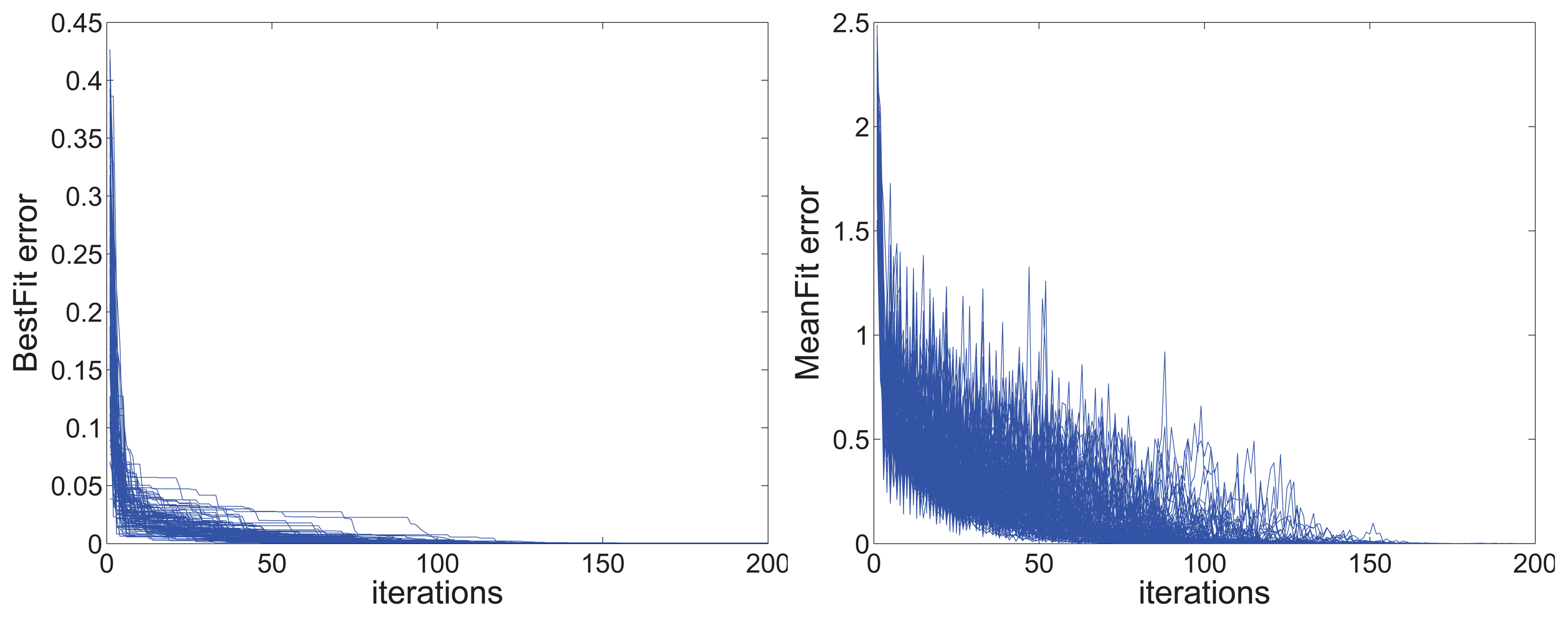
This algorithm must ensure that the iteration is stably convergent. To demonstrate its feasibility, the random data are used to test the convergence of the algorithm. One hundred cases are used to test the average iteration number and the rate of convergence, the results are shown in Figure 13. Just as the figure shows, the proposed method works well in different cases. It is obvious that the convergence of error in the individual best position and the global best position can meet the requirement with less than 200-times the iterations.
Take the 100 particles group, for example; a 200-times iteration means 20,000 particles are calculated. Compared to the calculated amount of directly calculating the iteration, the proposed approach has the advantage of fast speed and high feasibility.
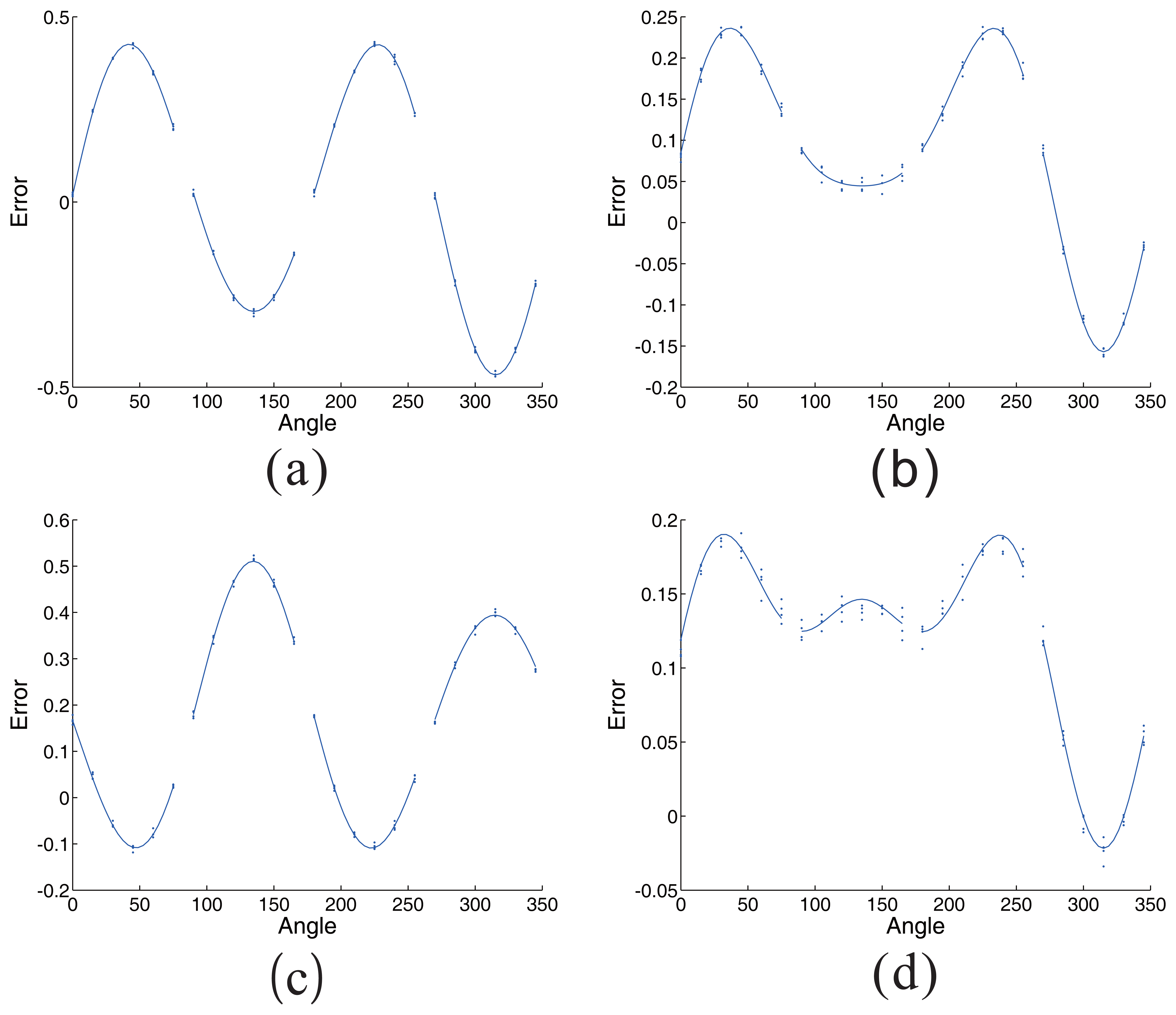
For the sensors working in different environment, there are many shapes of error. As shown in Table 2, the variables related to factors are variable in a range. The output error parameters in different situations (a, b, c, d) are demonstrated in the table. The different error shapes, related to the output error parameters, are respectively shown in Figure 14. The situations (a, b, c, d) in Table 2 are corresponding to the (a), (b), (c), (d) in Figure 14. Thereinto, the discrete points are four groups measuring errors in the same situation, while the curves are drawn using the output error parameters.
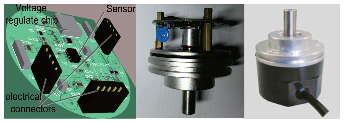
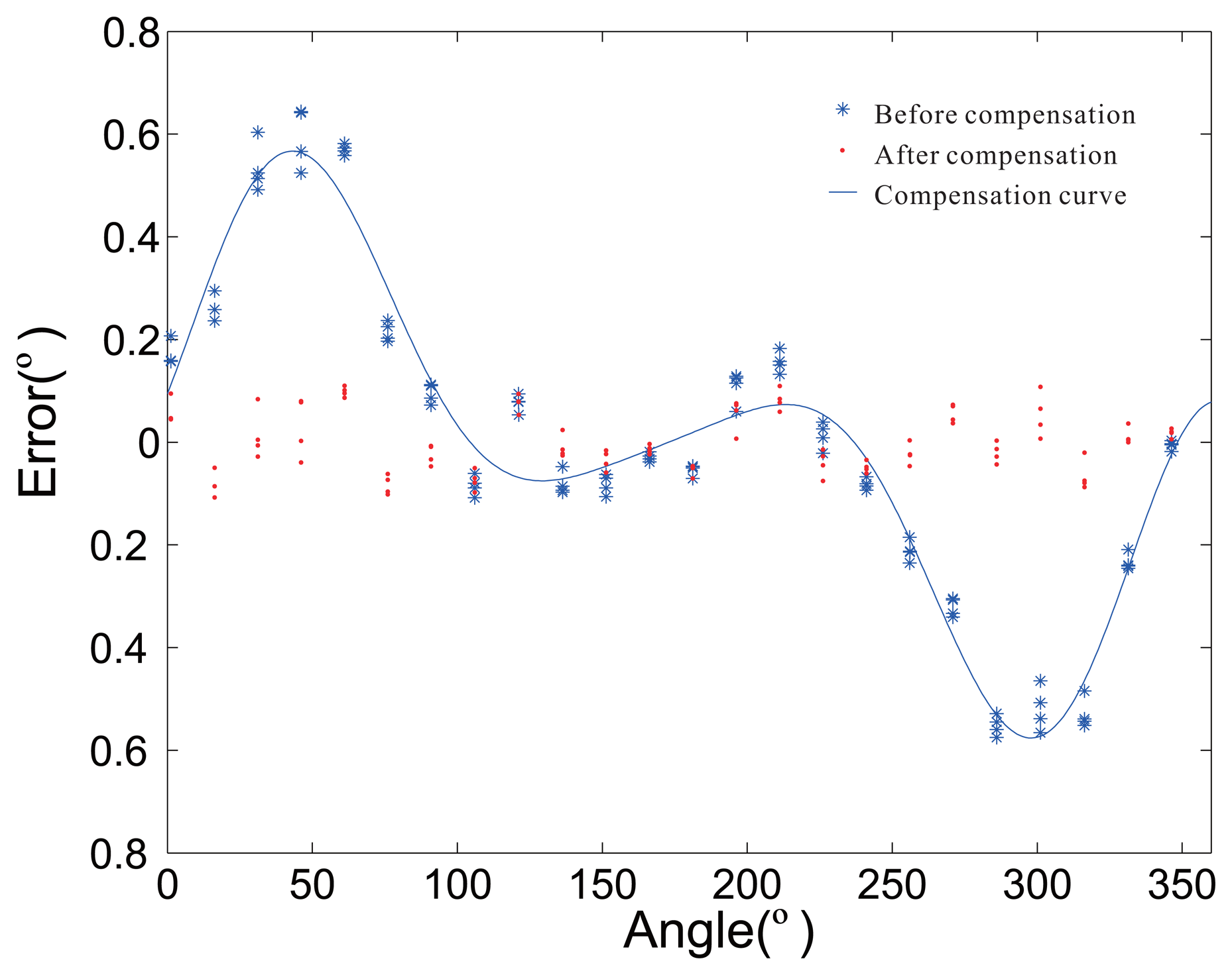
Although there is not strictly a one-to-one relationship to the real situation, the parameters can reflect the changing trend of the working condition. Using the parameters, small changes during the manufacturing process can be monitored. Additional, the back-end compensation parameters can be changed from the discontinuity point to the continuity curve. The printed circuit board (PCB) and real product photos are presented in Figure 15. The error distribution before and after the compensation are shown in Figure 16. After error compensation, the accuracy of the rotary encoder reaches 0.2°, and it has the same accuracy within the scope of the whole cycle.
5. Conclusions and Future Works
The analysis of factors is very important to improve the performance of Hall devices, which provides guidance to the designing and manufacturing process of rotary encoders. In this paper, a model-based rapid diagnosis method for rotary encoders based on Hall plates with a magnetic concentrator is proposed. The parameters of error factors in the possible range are used to fit the error curve by comparing the minimum residual angle error. Meanwhile, the modified PSO algorithm is used to improve the calculation speed.
Using this method, the parameters of the error can be obtained without using high-cost internal measurement. The parameters can reflect the trend of the error factor change and provide an easy way to get error factors after the assembly of the encoder. Using the parameters, small changes during the manufacturing process can be monitored. By keeping the sensor in good working condition, such as a least non-linear distance in different magnet and distance cases, as well as continuous error compensating, this keeps the accuracy in the whole cycle close to an agreement. The method by calculating the results to back-step the presence or absence of error is easier and more effective. Compared to the traditional measuring method, the model-based diagnosis method is a more effective way to locate error factors.
For all of that, the model and error locating method are not perfect; because some factors are sensitive to temperature, while some factors are immune to it. Selective compensation of the parameters can help the temperature characteristics [26,30]. In the future, the models taking into account more factors and the corresponding error, and therefore being more accurate, will be the focus of further work.
Acknowledgments
This work has been co-supported by The National High Technology Research and Development of China 863 Program (2012AA111004, 2012AA112312) and National Natural Science Foundation of China (61104088, 61175075, 61203019).
Author Contributions
Bumin Meng, Yaonan Wang, Wei Sun designed the study. Bumin Meng and Xiaofang Yuan analyzed the data and carried out the model-based rapid diagnosis method. Bumin Meng and Wei Sun performed the experiments. Yaonan Wang managed the funding, prepared the manuscript and supervised the whole project. Bumin Meng, Yaonan Wang, Wei Sun and Xiaofang Yuan wrote the manuscript. All of the authors read and approved the final manuscript.
Conflicts of Interest
The authors declare no conflict of interest.
References
- Lequesne, B.; Schroeder, T. High accuracy magnetic position encoder concept. Proceedins of the The 1998 IEEE Thirty-Third IAS Annual Meeting, St. Louis, MO, USA, 12–15 October 1998; pp. 187–196.
- Ripka, P.; Janosek, M. Advances in Magnetic Field Sensors. IEEE Sens. J. 2010, 10, 1108–1116. [Google Scholar]
- Lenz, J.E. A review of magnetic sensors. Proc. IEEE 1990, 78, 973–989. [Google Scholar]
- Lenz, J.; Edelstein, S. Magnetic sensors and their applications. IEEE Sens. J. 2006, 6, 631–649. [Google Scholar]
- Sriratana, W.; Murayama, R.; Tanachaikhan, L. Application of the HES in Angular Analysis. J. Sens. Technol. 2012, 2, 87–93. [Google Scholar]
- Ellin, A.; Dolsak, G. The design and application of rotary encoders. Sens. Rev. 2008, 28, 150–158. [Google Scholar]
- Popovic, R.; Schott, C. Magnetic Field Direction Sensor for Angle Indicator, Using Magnetic Field Sensor Elements Arranged Along at Least 3 Measuring Axes. U.S. Patent 7235968-B2, 26 November 2006. [Google Scholar]
- Taylor, W.P. Integrated Sensor Having a Magnetic Flux Concentrator. U.S. Patent 7,476,953, 13 January 2009. [Google Scholar]
- Bilotti, A.; Monreal, G.; Vig, R. Monolithic magnetic Hall sensor using dynamic quadrature offset cancellation. IEEE J. Solid-State Circuits 1997, 32, 829–836. [Google Scholar]
- Udo, A. Limits of offset cancellation by the principle of spinning current Hall probe. Proceedings of the IEEE Sensors, Vienna, Austria, 24–27 October 2004; Volume 3, pp. 1117–1120.
- Haberli, A.; Schneider, M.; Malcovati, P.; Castagnetti, R.; Maloberti, F.; Baltes, H. Two-dimensional magnetic microsensor with on-chip signal processing for contactless angle measurement. IEEE J. Solid-State Circuits 1996, 31, 1902–1907. [Google Scholar]
- Demierre, M.; Schurig, E.; Schott, C.; Besse, P.-A.; Popovicć, R.S. Contactless 360° absolute angular CMOS microsystem based on vertical Hall sensors. Sens. Actuators A Phys. 2004, 116, 39–44. [Google Scholar]
- Schott, C.; Waser, J.-M.; Popovic, R.S. Single-chip 3-D silicon Hall sensor. Sens. Actuators A Phys. 2000, 82, 167–173. [Google Scholar]
- Drljaca, P.M.; Demierre, M.; Schott, C.; Popovic, R.S. Nonlinear effects in magnetic angular position sensor with integrated flux concentrator. Proceedinngs of the 23rd International Conference on Microelectronics, Nis, Yugoslavia, 12–15 May 2002; Volume 1, pp. 223–226.
- Schott, C.; Besse, P.-A.; Popovic, R.S. Planar Hall effect in the vertical Hall sensor. Sens. Actuators A Phys. 2000, 85, 111–115. [Google Scholar]
- Ravaud, R.; Lemarquand, G.; Lemarquand, V.; Depollier, C. Analytical Calculation of the Magnetic Field Created by Permanent-Magnet Rings. IEEE Trans. Magnet. 2008, 44, 1982–1989. [Google Scholar]
- Huiser, A.M.J.; Baltes, H.P. Numerical modeling of vertical Hall-effect devices. IEEE Electron Device Lett. 1984, 5, 482–484. [Google Scholar]
- Schott, C.; Racz, R.; Manco, A.; Simonne, N. CMOS single-chip electronic compass with microcontroller. IEEE J. Solid-State Circuits 2007, 42, 2923–2933. [Google Scholar]
- Schott, C.; Racz, R.; Huber, S. Smart CMOS sensors with integrated magnetic concentrators. Proceedings of the 2005 IEEE Sensors, Irvine, CA, USA, 30 October–3 November 2005; p. 4.
- Oppenheim, R.W.S.A.V.; Buck, J.R. Discrete-Time Signal Processing, 2nd ed.; Prentice-Hall: Upper Saddle River, NJ, USA, 1999. [Google Scholar]
- Bendat, J.S.; Piersol, A.G. Random Data Analysis and Measurement Procedures. Meas. Sci. Technol. 11. [CrossRef]
- Tang, P.T.P. Table-lookup algorithms for elementary functions and their error analysis. Proceedings of the 10th IEEE Symposium on Computer Arithmetic, Grenoble, France, 26–28 June 1991; pp. 232–236.
- Antelo, E.; Bruguera, J.D.; Lang, T.; Zapata, E.L. Error analysis and reduction for angle calculation using the CORDIC algorithm. IEEE Trans. Comput. 1997, 46, 1264–1271. [Google Scholar]
- Volder, J.E. The CORDIC Trigonometric Computing Technique. IRE Trans. Electron. Comput. 1959, 8, 330–334. [Google Scholar]
- Meher, P.K.; Valls, J.; Juang, T.-B.; Sridharan, K.; Maharatna, K. 50 Years of CORDIC: Algorithms, Architectures, and Applications. IEEE Trans. Circuits Syst. I: Regul. Pap. 2009, 56, 1893–1907. [Google Scholar]
- Ausserlechner, U. Inaccuracies of Giant Magneto-Resistive Angle Sensors Due to Assembly Tolerances. IEEE Trans Magnet. 2009, 45, 2165–2174. [Google Scholar]
- Kennedy, J.; Eberhart, R. Particle swarm optimization. Proceedings of the IEEE International Conference on Neural Networks, Perth, WA, USA, 27 November–1 December 1995; Volume 4, pp. 1942–1948.
- Shi, Y.; Eberhart, R. A modified particle swarm optimizer. Proceedings of the 1998 IEEE International Conference on Evolutionary Computation, Anchorage, AK, USA, 4–9 May 1998; pp. 69–73.
- Van den Bergh, F. An Analysis of Particle Swarm Optimizers. Ph.D. Thesis, University of Pretoria, Pretoria, South Africa, 2006. [Google Scholar]
- Tsiantos, V.; Schrefl, T.; Scholz, W.; Forster, H.; Suess, D.; Dittrich, R.; Fidler, J. Thermal fluctuations in magnetic sensor elements. Sens. Actuators A Phys. 2003, 106, 134–136. [Google Scholar]


| Factor | Calculated Error | Impact Factor |
|---|---|---|
| Offset | 0.08102 | 1 mV offset in both axes |
| Gain mismatch | 0.08581 | mismatch ratio is 0.003 |
| Phase | 0.09999 | phase deviation is 0.1° |
| Non-Linearity | 0.07682 | magnetic field intensity is 100 mT |
| Voltage Fluctuation | 0.072 | 1 mV fluctuation in max impact |
| Calculation Error | 0.0078 | 8 times iterations with the worst case |
| Other | immeasurable | Other factors |
| Sum Foreseeable | 0.42346 | not including immeasurable factors |
Note: The calculated error is in degrees. The calculated error is the max value of the situation. As you can see, the sum value is unacceptable. To improve the performance of the sensor, we must control these factors within a rational range.
| Factor | Definition of Parameters | Output of Parameters | ||||||
|---|---|---|---|---|---|---|---|---|
| Variable | Range (min) | Range (max) | Step | a | b | c | d | |
| Offset | Vx | −0.01 | 0.01 | 0.000001 | 0.008943 | 0.005878 | 0.007500 | 0.007711 |
| mismatch | Ax | 0.99 | 1.01 | 0.000001 | 1.008607 | 1.000057 | 0.993573 | 0.994878 |
| Offset | Vy | −0.01 | 0.01 | 0.000001 | 0.000491 | 0.007176 | −0.006990 | −0.003980 |
| mismatch | Ay | 0.99 | 1.01 | 0.000001 | 0.994536 | 0.995089 | 1.003337 | 0.992822 |
| Phase | Px | −0.9/pi | 0.9/pi | 0.00009/pi | 0.000368 | 0.001508 | 0.003005 | 0.002122 |
| Linearity | Magx | 50 | 150 | 1 | 113 | 135 | 71 | 110 |
Note: The step and range of parameters are given as the above table. Using the diagnostic method, parameters in different situations can be obtained.
© 2014 by the authors; licensee MDPI, Basel, Switzerland. This article is an open access article distributed under the terms and conditions of the Creative Commons Attribution license ( http://creativecommons.org/licenses/by/3.0/).
Share and Cite
Meng, B.; Wang, Y.; Sun, W.; Yuan, X. A Novel Diagnosis Method for a Hall Plates-Based Rotary Encoder with a Magnetic Concentrator. Sensors 2014, 14, 13980-13998. https://doi.org/10.3390/s140813980
Meng B, Wang Y, Sun W, Yuan X. A Novel Diagnosis Method for a Hall Plates-Based Rotary Encoder with a Magnetic Concentrator. Sensors. 2014; 14(8):13980-13998. https://doi.org/10.3390/s140813980
Chicago/Turabian StyleMeng, Bumin, Yaonan Wang, Wei Sun, and Xiaofang Yuan. 2014. "A Novel Diagnosis Method for a Hall Plates-Based Rotary Encoder with a Magnetic Concentrator" Sensors 14, no. 8: 13980-13998. https://doi.org/10.3390/s140813980
APA StyleMeng, B., Wang, Y., Sun, W., & Yuan, X. (2014). A Novel Diagnosis Method for a Hall Plates-Based Rotary Encoder with a Magnetic Concentrator. Sensors, 14(8), 13980-13998. https://doi.org/10.3390/s140813980